Approximate analytical solutions and applications of pantograph-type equations with Caputo derivative and variable orders

Abstract

This study presents an efficient method that is suitable for differential equations, both with integer-order and fractional derivatives. This study examines the construction of solutions of fractional differential equations that are associated with varying delay proportional to the independent variable using a hybrid of Sumudu transform method. This study considers differential equations with Caputo derivatives of fractional variable orders and their applications in Nuclear Physics. The application indicates that fractional differential equations that have varying delay proportional to the independent variable are useful as tools for the modelling of many anomalous phenomena in nature and in the theory of complex systems.

Keywords:

• Sumudu transform
• hybrid
• pantograph
• Caputo derivatives
• model

Abbreviations:

• ODE: ordinary differential equation
• HSV: hybrid Sumudu variational
• ST:Sumudu transform

2010 MATHEMATICS SUBJECT CLASSIFICATIONS:

• 34A08
• 34A25
• 81V35

1. Introduction

The concept of fractional calculus provides a platform for generalization of differentiation to non-integer orders. Modelling problems that involve the notion of non-locality and memory effect, which are not well elucidated by integer-order operators are succinctly described by the fractional derivative operators (see, e.g. [1]). Fractional calculus provides a platform through which it is possible to debate various kinds of questions including viscoelastic systems and electrode–electrolyte polarization that are modelled by fractional equations (see, e.g. [2]). It is possible in some cases for the state of a system to be determined not by its entire history, but through its current moment and certain moment in the past. Such a system is referred to as a delay system. Delays are inherently bonded with several dynamical systems. There are cases where delays are functions of time t, and it is expressed as $\tau =\tau \left(t\right),$ with $\tau \left(t\right)>0$ (see, e.g. [3]). Consider a first-order linear Ordinary Differential Equation (ODE) that is associated with varying delay proportional to the independent variable (1) $y^{\prime }\left(t\right)=f(t,y_i(t),y_i(\lambda t\left)\right),$(1) where $i=1,2,3,\dots ,n$ and $\lambda >0(\lambda \ne 1)$ is referred to as pantograph equation. For $0<\lambda <1,$ (1(1) $y^{\prime }\left(t\right)=f(t,y_i(t),y_i(\lambda t\left)\right),$(1) ) is a special case of delay differential equations that has varying delay $\tau \left(t\right)=(1-\lambda )t.$ Equation (1(1) $y^{\prime }\left(t\right)=f(t,y_i(t),y_i(\lambda t\left)\right),$(1) ) models the dynamics of a current collection system for an electric locomotive [4]. Pantograph equations are involved in mathematical modelling of various processes in electrodynamics [5], population theory [6,7], number theory [8], stochastic games [9], graph theory [10], risk and queue theory [11] and theory of neural networks [12]. Hence, efforts on methods of solving pantograph-type equations are well justified (see, e.g. [13,14]). Solving pantograph-type ODE by using approximate analytical and numerical methods can be considered fairly well developed. Studies on the construction of approximate analytical solutions of pantograph-type ODEs and their analysis are contained, for example, in [4,15–18]. Obtaining the solutions of such equations by using the numerical methods are carried out in [19–21]. Those methods are fine if obtaining an approximate solution is the objective because they rarely give exact solutions. For an improvement in the solutions of differential equations, contemporary studies have considered the use of some new numerical and analytical techniques (see, e.g. [22–26]). Integer-order differential operators are not always enough to model the processes with memory effects. Fractional-order differential operators are more preferred than the integer-order differential operators in describing several physical phenomena (see, e.g. [27]). Treatments of fractional differential equations have been considered by using Time Scale Method (TSM) for numerical solutions (see, e.g. [28–30]) and Neural Network (NN) method (see, e.g. [31,32]). The impediment to using the TSM for solving pantograph-type equations is that it requires that the delay term is evaluated in every step (see, e.g. [33]). The impediment can lead to either an increase in the computational cost or a reduction of the overall accuracy of the numerical scheme. When compared with standard numerical methods, the NN-based solutions are preferred because they feature specific advantages such as being differentiable and has a closed analytic form (see, e.g. [33–36]). However, it is paradox that there are cases where one can prove the existence of NN-based solution with great approximation qualities for basic well-conditioned problems in scientific computing but there does not exist any algorithm, even randomized, that can train (or compute) such an NN [37]. The integral transform methods such as Laplace Transform (LT), ρ-Laplace transform are widely remarked as effective methods that lead to the exact solution for linear ODEs/PDEs (see, e.g. [38–43]). This gives the LT a relative advantage over other methods that are listed above in treating mathematical models. A simple modified form of LT is the Sumudu Transform (ST). Like the well-known LT, the ST is an integral method. For each property of LT, corresponding property can be obtained for ST (see, e.g. [44–46]). Applications of ST in solving various forms of differential equations are considered in [47–50]. Using ST technique is appealing as it yields an accurate result quickly and it does not impose any assumption that might restrict the solutions.

The aim of this study is to introduce a scheme that is efficient in accuracy and computational time. This paper considers pantograph-type equations with fractional derivatives. This paper presents a hybrid of ST method for solving pantograph-type equations with Caputo derivatives of fractional variable orders. It considers a problem in Nuclear Physics by presenting an analysis of the operation of nuclear reactors. ${}^{135}I$ produces an artificial element that has a great influence on a nuclear reactor operation (see, e.g. [51,52]). This paper proposes a model with Caputo derivative of fractional variable orders and a model of pantograph-type with Caputo derivative of fractional variable orders, which are analogues of an existing model with integer-order derivative operators. Finally, this paper presents the graphs of solutions for each model.

2. Preliminaries

In this section, the definition of the terms is given as applicable to this study. In addition, we state some existing results that are relevant to this study. Throughout this paper, the set of real and natural numbers will be denoted by $\mathbb{R}$ and $\mathbb{N},$ respectively.

Definition 2.1

Consider $\mathrm{\Lambda }=\left\{y\right(t):\mathrm{\exists }Q,{\xi }_1,{\xi }_2>0,|y(t)|<Q{e}^{|t|/{\xi }_j},\text{if}t\in (-1{)}^j\times [0,\mathrm{\infty })\},$ which is a set of functions (see, e.g. [44]). $y\left(t\right)\in \mathrm{\Lambda }$ for all real $t\ge 0.$ The ST for a given function $I\left(t\right)$ will be denoted by $\mathcal{S}\left[y\right(t\left)\right]=Y\left(u\right),$ defined as (2) $Y\left(u\right):=\mathcal{S}\left[y\right(t\left)\right]={\int }_0^{\mathrm{\infty }}y\left(tu\right)e^{-t}\mathrm{d}t,u\in (-{\xi }_1,{\xi }_2).$(2) The inverse ST of $Y\left(u\right)$ in Equation (2(2) $Y\left(u\right):=\mathcal{S}\left[y\right(t\left)\right]={\int }_0^{\mathrm{\infty }}y\left(tu\right)e^{-t}\mathrm{d}t,u\in (-{\xi }_1,{\xi }_2).$(2) ) is the function $y\left(t\right).$ ST is an integral method like the well-known Laplace transform, defined as (3) $L\left(u\right):=\mathcal{L}\left[y\right(t\left)\right]={\int }_0^{\mathrm{\infty }}y\left(t\right)e^{-st}\mathrm{d}t,s>0,$(3) for a given function $y\left(t\right).$ It can be observed from Equations (2(2) $Y\left(u\right):=\mathcal{S}\left[y\right(t\left)\right]={\int }_0^{\mathrm{\infty }}y\left(tu\right)e^{-t}\mathrm{d}t,u\in (-{\xi }_1,{\xi }_2).$(2) ) and (3(3) $L\left(u\right):=\mathcal{L}\left[y\right(t\left)\right]={\int }_0^{\mathrm{\infty }}y\left(t\right)e^{-st}\mathrm{d}t,s>0,$(3) ) that the duality relations between ST and Laplace transform are given as $Y\left(1/s\right)=sL\left(s\right),L\left(1/u\right)=uY\left(u\right).$ ST is very efficient in obtaining a Lagrange multiplier. ST is very quick in yielding an accurate result and it does not impose any restriction on the results. ST satisfies linear property (see, e.g. [44–46,53]). Indeed, for arbitrary two given functions $y\left(t\right),z\left(t\right)\in \mathrm{\Lambda },$ and for arbitrary constants θ and ζ, $\mathcal{S}\left[\theta y\right(t)+\zeta z(t\left)\right]=\theta \mathcal{S}\left[y\right(t\left)\right]+\zeta \mathcal{S}\left[z\right(t\left)\right].$ For an integer-order derivative, its ST is expressed as (4) $S\left[\frac{\mathrm{d}y\left(t\right)}{\mathrm{d}t}\right]=\frac{1}{u}\left[Y\right(u)-y(0\left)\right],$(4) and it is given as (5) $S\left[\frac{d^{n}y\left(t\right)}{\mathrm{d}{t}^n}\right]=\frac{1}{u^n}\left[Y\right(u)-\sum _{k=0}^{n-1}{u}^k\frac{d^{k}y\left(t\right)}{\mathrm{d}{t}^k}{|}_{t=0}],$(5) for the nth-order derivative.

The following established results give information about the existence and convergence of the ST (see, e.g, [54]).

Lemma 2.2

Existence

If y is an exponential order, then its ST $\mathcal{S}\left[y\right(t),u]=Y\left(u\right)$ is given by $Y\left(u\right)=\frac{1}{u}{\int }_{-\mathrm{\infty }}^{\mathrm{\infty }}{e}^{(-t/u)}y\left(t\right)\mathrm{d}t,$ where $1/u=1/\varphi +i/\phi .$ The defining integral for X exists at points $1/u=1/\varphi +i/\phi ,\varphi ,\phi \in \mathbb{R}.$

Lemma 2.3

Uniqueness

Let $y\left(t\right)$ and $z\left(t\right)$ be continuous functions defined for $t\ge 0$ and whose Sumudu transforms are $Y\left(u\right)$ and $Z\left(u\right),$ respectively. If $Y\left(u\right)=Z\left(u\right)$ almost everywhere, then $y\left(t\right)=z\left(t\right),$ where u is a complex number.

Lemma 2.4

Convergence

Let $y\left(t\right)$ be a continuous function. If the integral $\frac{1}{u}{\int }_0^{\mathrm{\infty }}{e}^{(-t/u)}y\left(t\right)\mathrm{d}t$ converges at $u=u_0,$ then the integral converges for $u<u_0.$

Definition 2.5

Let a>0, b>0 be positive real numbers. The left- and right-sided Caputo-fractional derivatives are defined respectively for order α as ${}_a^C{D}^{\alpha }y\left(t\right)=\frac{1}{\mathrm{\Gamma }(1-\alpha )}{\int }_a^t(t-\xi {)}^{-\alpha }{y}^{\prime }(\xi )\mathrm{d}\xi$ and ${}^C{D}_b^{\alpha }y\left(t\right)=\frac{-1}{\mathrm{\Gamma }(1-\alpha )}{\int }_t^b(\xi -t{)}^{\alpha }{y}^{\prime }(\xi )\mathrm{d}\xi ,$ where $0<\alpha <1$ (see, e.g. [44] , Theorems 4.1 and 4.2). Consequently, the ST for Caputo-fractional derivatives of order α has the form (see, e.g. [27]) (6) $\mathcal{S}\left[{}_0^C{D}^{\alpha }y\right(t\left)\right]=u^{-\alpha }(\mathcal{S}\left[y\right(t\left)\right]-y(0\left)\right).$(6)

Table 1 gives the list of some special ST.

Table 1. Special Sumudu transform.

$y\left(t\right)$	$Y\left(u\right):=\mathcal{S}\left[y\right(t\left)\right]$
1	1
t	u
${\displaystyle \frac{t^n}{n!}}$	$u^n$
$e^{at}$	${\displaystyle \frac{1}{1-au}}$
${\displaystyle \frac{sinat}{a}}$	${\displaystyle \frac{u}{1+a^2{u}^2}}$
$cosat$	${\displaystyle \frac{1}{1+a^2{u}^2}}$
${\displaystyle \frac{e^{bt}-e^{at}}{b-a}},b\ne a$	${\displaystyle \frac{1}{(1-bu)(1-au)}}$

Proposition 2.6

Let $\varphi ,\phi :[0,\mathrm{\infty })\to \mathbb{R},$ then the classical convolution product is given by $(\varphi \times \psi )\left(t\right)={\int }_0^t\varphi (t-x)\psi \left(x\right)\mathrm{d}x.$ The ST for the convolution product is given by $\begin{array}{rl}\mathcal{S}\left[\right(\varphi \times \psi \left)\right(t\left)\right]& =u\mathcal{S}\left[\varphi \right(t\left)\right]\mathcal{S}\left[\psi \right(t\left)\right]\\ & =u\varphi \left(u\right)\psi \left(u\right).\end{array}$

Definition 2.7

The Mittag–Leffler function $E_{\alpha }\left(t\right)$ is defined as $E_{\alpha }\left(t\right)=\sum _{n=0}^{\mathrm{\infty }}{t}^n/\left(n\alpha \right)!,\alpha >0.$ The following results about Mittag–Leffler functions and ST are well known (see, e.g. [55]):

1. $\mathcal{S}\left[E_{\alpha }\right(-a{t}^{\alpha }\left)\right]=\frac{1}{1+a{u}^{\alpha }};$

2. $\mathcal{S}[1-E_{\alpha }(-a{t}^{\alpha }\left)\right]=\frac{a{u}^{\alpha }}{1+a{u}^{\alpha }}.$

3. Main results

This study considers how to use a hybrid of variational iterative method with ST to obtain the solutions of differential equations of pantograph type with Caputo derivatives of fractional variable orders. The Caputo derivative is a notable fractional operator that is most appropriate in the modelling of real-world problems. We show the application of the results of this study by considering a problem in Nuclear Physics.

3.1. Hybrid Sumudu variational (HSV) method

In this study, the Hybrid Sumudu Variational (HSV) method will refer to a union of variational iterative methods with ST. Choosing variational iterative method as the most suitable companion for amalgamation with the ST is due to the fact that variational iterative method has been remarkable for its flexibility, consistency and effectiveness (see, e.g. [56,57] and references there in).

3.1.1. Demonstration of HSV method

Interest in the Caputo derivative as a notable fractional operator is due to the important roles that it play in the modelling of real-life phenomena. The Caputo derivative of fractional variable order is the most suitable for a model where the attention given to the interactions within the past and also problems with nonlocal properties (see, e.g. [58]). We present how to use the HSV method to solve a most general form of pantograph differential equations with Caputo derivatives of fractional variable orders (7) ${}_a^C{D}^{\alpha }y\left(t\right)+\mathrm{\Phi }\left[y\right(t\left)\right]+\mathrm{\Psi }\left[y\right(\lambda t\left)\right]=\omega \left(t\right)$(7) that possesses the initial conditions (8) $y\left(0\right)=y_0,$(8) where Φ and Ψ denote linear and nonlinear operators, respectively and $\omega \left(t\right)$ is a given continuous function. Take the ST of (7(7) ${}_a^C{D}^{\alpha }y\left(t\right)+\mathrm{\Phi }\left[y\right(t\left)\right]+\mathrm{\Psi }\left[y\right(\lambda t\left)\right]=\omega \left(t\right)$(7) ) to obtain $\mathcal{S}\left[{}_a^C{D}^{\alpha }y\right(t\left)\right]=\mathcal{S}\left[\omega \right(t)-\mathrm{\Phi }\left[y\right(t\left)\right]+\mathrm{\Psi }\left[y\right(\lambda t\left)\right]].$ Apply (6(6) $\mathcal{S}\left[{}_0^C{D}^{\alpha }y\right(t\left)\right]=u^{-\alpha }(\mathcal{S}\left[y\right(t\left)\right]-y(0\left)\right).$(6) ) with $a=0,$ we obtain $u^{-\alpha }(\mathcal{S}\left[y\right(t\left)\right]-y(0\left)\right)=\mathcal{S}\left[\omega \right(t)-\mathrm{\Phi }\left[y\right(t\left)\right]-\mathrm{\Psi }\left[y\right(\lambda t\left)\right]].$ Recall that it is given that $y\left(0\right)=y_0$ by (8(8) $y\left(0\right)=y_0,$(8) ), therefore $u^{-\alpha }\left(Y\right(u)-y_0)=\mathcal{S}\left[\omega \right(t)-\mathrm{\Phi }\left[y\right(t\left)\right]-\mathrm{\Psi }\left[y\right(\lambda t\left)\right]].$ Consequently, the HSV formula is obtained as (9) $Y_{n+1}\left(u\right)=Y_n\left(u\right)+\varphi \left(u\right)(\frac{Y_n\left(u\right)-y_0}{u^{\alpha }}-\mathcal{S}\left[\omega \right(t)-\mathrm{\Phi }\left[y\right(t\left)\right]-\mathrm{\Psi }\left[y\right(\lambda t\left)\right]]),n\in \mathbb{N}.$(9) Considering $\mathcal{S}\left[\mathrm{\Phi }\right[y\left(t\right)]-\mathrm{\Psi }[y\left(\lambda t\right)\left]\right]$ as the restricted term and taking the classical variation operator on both sides of (9(9) $Y_{n+1}\left(u\right)=Y_n\left(u\right)+\varphi \left(u\right)(\frac{Y_n\left(u\right)-y_0}{u^{\alpha }}-\mathcal{S}\left[\omega \right(t)-\mathrm{\Phi }\left[y\right(t\left)\right]-\mathrm{\Psi }\left[y\right(\lambda t\left)\right]]),n\in \mathbb{N}.$(9) ) gives $\delta Y_{n+1}\left(u\right)=\delta Y_n\left(u\right)+\varphi \left(u\right)\frac{1}{u^{\alpha }}\delta Y_n\left(u\right),$ and Lagrange multiplier as (10) $\varphi \left(u\right)=-u^{\alpha }.$(10) Substitute (10(10) $\varphi \left(u\right)=-u^{\alpha }.$(10) ) into (9(9) $Y_{n+1}\left(u\right)=Y_n\left(u\right)+\varphi \left(u\right)(\frac{Y_n\left(u\right)-y_0}{u^{\alpha }}-\mathcal{S}\left[\omega \right(t)-\mathrm{\Phi }\left[y\right(t\left)\right]-\mathrm{\Psi }\left[y\right(\lambda t\left)\right]]),n\in \mathbb{N}.$(9) ) and then take its inverse ST to obtain $\begin{array}{rl}{y}_{n+1}\left(t\right)& =y_n\left(t\right)+{\mathcal{S}}^{-1}[-u^{\alpha }(\frac{Y_n\left(u\right)-y_0}{u^{\alpha }}-\mathcal{S}\left[\omega \right(t)-\mathrm{\Phi }\left[y_n\right(t\left)\right]-\mathrm{\Psi }\left[y_n\right(\lambda t\left)\right]])]\\ & =y_1\left(t\right)+{\mathcal{S}}^{-1}\left[u^{\alpha }\mathcal{S}\left[\omega \right(t)-\mathrm{\Phi }\left[y_n\right(t\left)\right]-\mathrm{\Psi }\left[y_n\right(\lambda t\left)\right]]\right],\end{array}$ which is an explicit iteration formula with the initial approximation which is given as $y_1\left(t\right)={\mathcal{S}}^{-1}[-u^{\alpha }(\frac{-y_0}{u^{\alpha }}\left)\right]=y_0{\mathcal{S}}^{-1}\left[1\right]=y_0.$

3.1.2. Differential equations of pantograph type with variable coefficients and Caputo derivatives of fractional variable orders

Consider differential equations of pantograph type with variable coefficients and Caputo derivatives of fractional variable orders of the form (11) ${}_a^C{D}^{\alpha }y\left(t\right)+\text{β}{\mathrm{\Phi }}_1\left[y\right(t\left)\right]+\psi \left(t\right){\mathrm{\Phi }}_2\left[y\right(t\left)\right]+\mathrm{\Psi }\left[y\right(\lambda t\left)\right]=\omega \left(t\right),$(11) where the coefficients β and $\psi \left(t\right)$ are a constant and a variable, respectively, ${\mathrm{\Phi }}_1$ and ${\mathrm{\Phi }}_2$ denote linear operators and other terms remain as defined in (7(7) ${}_a^C{D}^{\alpha }y\left(t\right)+\mathrm{\Phi }\left[y\right(t\left)\right]+\mathrm{\Psi }\left[y\right(\lambda t\left)\right]=\omega \left(t\right)$(7) ). Taking the ST of (11(11) ${}_a^C{D}^{\alpha }y\left(t\right)+\text{β}{\mathrm{\Phi }}_1\left[y\right(t\left)\right]+\psi \left(t\right){\mathrm{\Phi }}_2\left[y\right(t\left)\right]+\mathrm{\Psi }\left[y\right(\lambda t\left)\right]=\omega \left(t\right),$(11) ) and by similar computations as in Section 3.1.1, yields the HSV formula (12) $\begin{array}{rl}{Y}_{n+1}\left(u\right)& =Y_n\left(u\right)+\varphi \left(u\right)(\frac{Y_n\left(u\right)-y_0}{u^{\alpha }}-\mathcal{S}[\omega \left(t\right)-\text{β}{\mathrm{\Phi }}_1\left[y\right(t\left)\right]\\ & -\psi \left(t\right){\mathrm{\Phi }}_2\left[y\right(t\left)\right]-\mathrm{\Psi }\left[y\right(\alpha t\left)\right]]),n\in \mathbb{N}.\end{array}$(12) Considering $\mathcal{S}\left[\psi \right(t\left){\mathrm{\Phi }}_2\right[y\left(t\right)]+\mathrm{\Psi }[y\left(\lambda t\right)\left]\right]$ as the restricted term in taking the classical variation operator on both sides of (12(12) $\begin{array}{rl}{Y}_{n+1}\left(u\right)& =Y_n\left(u\right)+\varphi \left(u\right)(\frac{Y_n\left(u\right)-y_0}{u^{\alpha }}-\mathcal{S}[\omega \left(t\right)-\text{β}{\mathrm{\Phi }}_1\left[y\right(t\left)\right]\\ & -\psi \left(t\right){\mathrm{\Phi }}_2\left[y\right(t\left)\right]-\mathrm{\Psi }\left[y\right(\alpha t\left)\right]]),n\in \mathbb{N}.\end{array}$(12) ) yields $\delta Y_{n+1}\left(u\right)=\delta Y_n\left(u\right)+\varphi \left(u\right)\frac{1}{u^{\alpha }}\delta Y_n\left(u\right),$ and consequently the Lagrange multiplier as $\varphi \left(u\right)=-u^{\alpha }.$ Substituting for $\varphi \left(u\right)$ in (12(12) $\begin{array}{rl}{Y}_{n+1}\left(u\right)& =Y_n\left(u\right)+\varphi \left(u\right)(\frac{Y_n\left(u\right)-y_0}{u^{\alpha }}-\mathcal{S}[\omega \left(t\right)-\text{β}{\mathrm{\Phi }}_1\left[y\right(t\left)\right]\\ & -\psi \left(t\right){\mathrm{\Phi }}_2\left[y\right(t\left)\right]-\mathrm{\Psi }\left[y\right(\alpha t\left)\right]]),n\in \mathbb{N}.\end{array}$(12) ) and taking its inverse ST yields

$\begin{array}{rl}& y_{n+1}\left(t\right)\\ & =y_n\left(t\right)+{\mathcal{S}}^{-1}[-u^{\alpha }(\frac{Y_n\left(u\right)-y_0}{u^{\alpha }}-\mathcal{S}\left[\omega \right(t)-\text{β}{\mathrm{\Phi }}_1[y\left(t\right)]-\psi (t\left){\mathrm{\Phi }}_2\right[y\left(t\right)]-\mathrm{\Psi }\left[y\right(\lambda t\left)\right]])]\\ & =y_1\left(t\right)+{\mathcal{S}}^{-1}\left[u^{\alpha }\mathcal{S}\left[\omega \right(t)-\text{β}{\mathrm{\Phi }}_1[y\left(t\right)]-\psi (t\left){\mathrm{\Phi }}_2\right[y\left(t\right)]-\mathrm{\Psi }\left[y\right(\lambda t\left)\right]]\right],\end{array}$ which is an explicit iteration formula and where $y_1\left(t\right)={\mathcal{S}}^{-1}[-u^{\alpha }(\frac{-y_0}{u^{\alpha }}\left)\right]=y_0{\mathcal{S}}^{-1}\left[1\right]=y_0.$

3.2. Applications in nuclear physics

In Nuclear Physics, the atomic nucleus structure and propagation of radiation that emits from unstable nuclei are of particular interest. Some elements possess unstable nuclei. Such nuclei that are not stable are radioactive in nature. They radiate energy and particles, which are collectively referred to as radiation. A nuclear plant is composed of nuclear reactors (see, e.g. [52,59]). In Figure 1, the steel pressure vessel houses the whole reactor. A standard nuclear reactor that has uranium 235 as fuel element yields Xenon 135 (${}^{135}$Xe) as a result of fission. Little quantity of ${}^{135}$Xe is derived from fission (see, e.g. [60–62]). ${}^{135}$Xe is derived practically from the decay train Tellurium-135 (${}_{52}^{135}$Te) with ${\text{β}}^{-}$ decay and half-life of 19 sec to Iodine 135 (${}_{53}^{135}I$) with ${\text{β}}^{-}$ decay and half-life of 6.6 hr to ${}^{135}$Xe, that is (13) ${}_{52}^{135}\text{Te (with }{\text{β}}^{-}\text{ decay, half-life 19 sec)}⟶{}_{53}^{135}I\text{(with }{\text{β}}^{-}\text{ decay, half-life 6.6 hr)}⟶{}^{135}Xe.$(13) ${}^{135}$Xe has a considerable neutron-capture cross section (see, e.g. [51,63]). The Chain (13(13) ${}_{52}^{135}\text{Te (with }{\text{β}}^{-}\text{ decay, half-life 19 sec)}⟶{}_{53}^{135}I\text{(with }{\text{β}}^{-}\text{ decay, half-life 6.6 hr)}⟶{}^{135}Xe.$(13) ) indicates that ${}^{135}$Xe comes directly from the decay of ${}^{135}I.$ A model for the decay of ${}^{135}I$ is defined by the differential equation (14) $I^{\prime }\left(t\right)=\gamma -\rho I\left(t\right),$(14) where $I\left(t\right)$ represents the number of ${}^{135}I$ $\left({\text{atoms cm}}^{-3}\right),$ i.e. the atom density of iodine, ρ denotes the decay constant for ${}^{135}I$ and γ is a constant that denotes the product of thermal neutron flux, macroscopic fission cross-section and effective fission yield of the isotope (see, e.g. [64–66]). Solving the differential equation (14(14) $I^{\prime }\left(t\right)=\gamma -\rho I\left(t\right),$(14) ) yields the solution as (15) $I\left(t\right)=\gamma /\rho +\left(I\right(0)-\gamma /\rho )e^{-\rho t},$(15) where $I\left(0\right)$ refers to ${}^{135}I$ at the time $t=0.$ ${}^{135}I$ is said to be in equilibrium state when its rate of production and its rate of removal are equal. At equilibrium, ${}^{135}I$ undergoes complete decay to xenon and this state is described as the ${}^{135}$Xe reservoir. To determine the ${}^{135}I$ equilibrium concentration, setting $I^{\prime }\left(t\right)=0$ in (14(14) $I^{\prime }\left(t\right)=\gamma -\rho I\left(t\right),$(14) ) yields (16) $I\left(t\right)=\gamma /\rho ,$(16) which indicates that the concentration of ${}^{135}I$ remains constant at equilibrium. It can be deduced from (16(16) $I\left(t\right)=\gamma /\rho ,$(16) ) that the equilibrium concentration of ${}^{135}I$ varies with the fission reaction rate and consequently to the reactor power level. ${}^{135}I$ produces an artificial element that has a great influence on a nuclear reactor operation. On the decay of ${}^{135}I,$ this study considers two distinct models with Caputo derivatives of fractional variable orders. This study considers a model that does not associate with a delay and a model that is associated with delay.

Figure 1. A nuclear reactor [67].

3.2.1. Differential equations with Caputo derivatives of fractional variable orders for decay of ${}^{135}I$

Consider an analogue of (14(14) $I^{\prime }\left(t\right)=\gamma -\rho I\left(t\right),$(14) ) for the decay of ${}^{135}I$ that is given by a fractional differential equation with Caputo derivative of variable order (17) ${}_a^C{D}^{\alpha }I\left(t\right)=\gamma -\rho I\left(t\right),I\left(0\right)=I_0,$(17) where $\alpha \in (0,1).$ We shall apply ST method to solve (17(17) ${}_a^C{D}^{\alpha }I\left(t\right)=\gamma -\rho I\left(t\right),I\left(0\right)=I_0,$(17) ). Taking the ST of (17(17) ${}_a^C{D}^{\alpha }I\left(t\right)=\gamma -\rho I\left(t\right),I\left(0\right)=I_0,$(17) ) gives $\mathcal{S}\left[{}_a^C{D}^{\alpha }I\right(t\left)\right]=\gamma -\rho \mathcal{S}\left[I\right(t\left)\right],$ which results in $u^{-\alpha }(\mathcal{S}\left[I\right(t\left)\right]-I(0\left)\right)=\gamma -\rho \mathcal{S}\left[I\right(t\left)\right].$ It is given in (17(17) ${}_a^C{D}^{\alpha }I\left(t\right)=\gamma -\rho I\left(t\right),I\left(0\right)=I_0,$(17) ) that $I\left(0\right)=I_0.$ Therefore (18) $u^{-\alpha }\left(I\right(u)-I_0)=\gamma -\rho I\left(u\right).$(18) A simplification of (18(18) $u^{-\alpha }\left(I\right(u)-I_0)=\gamma -\rho I\left(u\right).$(18) ) gives (19) $\begin{array}{rl}I\left(u\right)& =\frac{u^{-\alpha }{I}_0+\gamma }{u^{-\alpha }+\rho }\\ & =\frac{u^{-\alpha }{I}_0}{u^{-\alpha }+\rho }+\frac{\gamma }{u^{-\alpha }+\rho }.\end{array}$(19) The inverse ST of (19(19) $\begin{array}{rl}I\left(u\right)& =\frac{u^{-\alpha }{I}_0+\gamma }{u^{-\alpha }+\rho }\\ & =\frac{u^{-\alpha }{I}_0}{u^{-\alpha }+\rho }+\frac{\gamma }{u^{-\alpha }+\rho }.\end{array}$(19) ) yields $\begin{array}{rl}I\left(t\right)& ={\mathcal{S}}^{-1}\left[\frac{u^{-\alpha }}{u^{-\alpha }+\rho }\right]I_0+{\mathcal{S}}^{-1}\left[\frac{\gamma }{u^{-\alpha }+\rho }\right]\\ & ={\mathcal{S}}^{-1}\left[\frac{1}{1+\rho u^{\alpha }}\right]I_0+\frac{\gamma }{\rho }{\mathcal{S}}^{-1}\left[\frac{\rho u^{\alpha }}{1+\rho u^{\alpha }}\right].\end{array}$ Consequently, by Definition 2.7 (i) and (ii), (20) $I\left(t\right)=I_0{E}_{\alpha }(-\rho t^{\alpha })+\gamma /\rho (1-E_{\alpha }(-\rho t^{\alpha })).$(20) Setting $\rho =0.3,\gamma =0.1,\alpha =0.85$ and $I_0=1,$ Figure 2 shows comparison between the solution given by (15(15) $I\left(t\right)=\gamma /\rho +\left(I\right(0)-\gamma /\rho )e^{-\rho t},$(15) ) for the model with integer-order derivative operator and solution given by (20(20) $I\left(t\right)=I_0{E}_{\alpha }(-\rho t^{\alpha })+\gamma /\rho (1-E_{\alpha }(-\rho t^{\alpha })).$(20) ) for the model with Caputo fractional derivative operator. 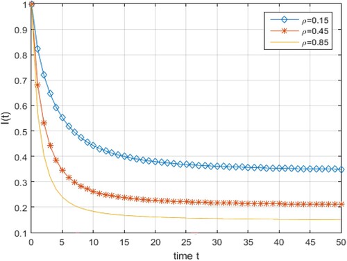Recall that $I_0$ signifies the value of ${}^{135}I$ at the time $t=0.$ In addition, setting $\rho =0.3$ and $\gamma =0.1,$ Figure 3 displays the effect that the variation of fractional order α, of the Caputo derivative operators has on the solution of the (17(17) ${}_a^C{D}^{\alpha }I\left(t\right)=\gamma -\rho I\left(t\right),I\left(0\right)=I_0,$(17) ). Moreover, setting $\gamma =0.1$ and $\alpha =0.85,$ Figure 4 shows how the solution given by (20(20) $I\left(t\right)=I_0{E}_{\alpha }(-\rho t^{\alpha })+\gamma /\rho (1-E_{\alpha }(-\rho t^{\alpha })).$(20) ) varies due to variation in ρ.

Figure 2. Comparison between model with integer-order derivative and model with Caputo fractional derivative operators.

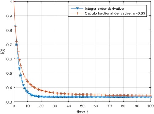
Figure 3. Effect of variation of order of Caputo fractional derivative operators.

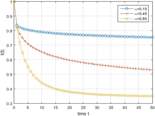
Figure 4. Variation in the solution given by (20(20) $I\left(t\right)=I_0{E}_{\alpha }(-\rho t^{\alpha })+\gamma /\rho (1-E_{\alpha }(-\rho t^{\alpha })).$(20) ) as ρ varies.

3.2.2. Differential equations with Caputo derivatives of fractional variable orders and time delay for decay of ${}^{135}I$

Consider an analogue of (17(17) ${}_a^C{D}^{\alpha }I\left(t\right)=\gamma -\rho I\left(t\right),I\left(0\right)=I_0,$(17) ) for the decay of ${}^{135}I$ that is given by a differential equation with Caputo derivative of fractional variable orders and a time delay (21) ${}_a^C{D}^{\alpha }I\left(t\right)=\gamma -\rho I\left(\lambda t\right),$(21) where $\alpha \in (0,1)$ and $I\left(0\right)=I_0.$

Remark 3.1

There is a clear difference between (17(17) ${}_a^C{D}^{\alpha }I\left(t\right)=\gamma -\rho I\left(t\right),I\left(0\right)=I_0,$(17) ) and (21(21) ${}_a^C{D}^{\alpha }I\left(t\right)=\gamma -\rho I\left(\lambda t\right),$(21) ) as delay is present in the latter. A mathematical model with a delay possesses more vitality and suitability for several real life phenomena. Observe that the solution of (17(17) ${}_a^C{D}^{\alpha }I\left(t\right)=\gamma -\rho I\left(t\right),I\left(0\right)=I_0,$(17) ) was obtained by using the ST method. Unfortunately, ST method is suitable for solving (21(21) ${}_a^C{D}^{\alpha }I\left(t\right)=\gamma -\rho I\left(\lambda t\right),$(21) ) due to the presence of a time delay in it. The HSV method that was presented in Section 3.1 will be applied to solve (21(21) ${}_a^C{D}^{\alpha }I\left(t\right)=\gamma -\rho I\left(\lambda t\right),$(21) ).

To apply HSV method, start by taking the ST of (21(21) ${}_a^C{D}^{\alpha }I\left(t\right)=\gamma -\rho I\left(\lambda t\right),$(21) ) with a = 0 to obtain $\mathcal{S}\left[{}_a^C{D}^{\alpha }I\right(t\left)\right]=\gamma -\rho \mathcal{S}\left[I\right(\lambda t\left)\right].$ Apply (6(6) $\mathcal{S}\left[{}_0^C{D}^{\alpha }y\right(t\left)\right]=u^{-\alpha }(\mathcal{S}\left[y\right(t\left)\right]-y(0\left)\right).$(6) ) to obtain $u^{-\alpha }(\mathcal{S}\left[I\right(t\left)\right]-I(0\left)\right)=\gamma -\rho \mathcal{S}\left[I\right(\lambda t\left)\right],$ which is equivalent to $u^{-\alpha }\left(I\right(u)-I_0)+\rho \mathcal{S}\left[I\right(\lambda t\left)\right]-\gamma =0,$ since $\mathcal{S}\left[I\right(t\left)\right]=I\left(u\right)$ and $I\left(0\right)=I_0.$ Therefore, the HSV iteration formula appears as (22) $I_{n+1}\left(u\right)=I_n\left(u\right)+\varphi \left(u\right)(\frac{I_n\left(u\right)-I_0}{u^{\alpha }}+\rho \mathcal{S}\left[I\right(\lambda t\left)\right]-\gamma ),n\in \mathbb{N}.$(22) $I\left(\lambda t\right)$ is considered as the restricted term in taking the classical variation operator on both sides of (22(22) $I_{n+1}\left(u\right)=I_n\left(u\right)+\varphi \left(u\right)(\frac{I_n\left(u\right)-I_0}{u^{\alpha }}+\rho \mathcal{S}\left[I\right(\lambda t\left)\right]-\gamma ),n\in \mathbb{N}.$(22) ). Then this yields $\varphi \left(u\right)=-u^{\alpha }.$

Substitute for $\varphi \left(u\right)$ in (22(22) $I_{n+1}\left(u\right)=I_n\left(u\right)+\varphi \left(u\right)(\frac{I_n\left(u\right)-I_0}{u^{\alpha }}+\rho \mathcal{S}\left[I\right(\lambda t\left)\right]-\gamma ),n\in \mathbb{N}.$(22) ) and take its inverse-ST to obtain $\begin{array}{rl}{I}_{n+1}\left(t\right)& =I_n\left(t\right)+{\mathcal{S}}^{-1}[-u^{\alpha }(\frac{I_n\left(u\right)-I_0}{u^{\alpha }}+\rho \mathcal{S}\left[I_n\right(\lambda t\left)\right]-\gamma )]\\ & =I_1\left(t\right)-{\mathcal{S}}^{-1}\left[u^{\alpha }(\rho \mathcal{S}\left[I_n\right(\lambda t\left)\right]-\gamma )\right],\end{array}$ which is an explicit iteration formula and where $I_1\left(t\right)={\mathcal{S}}^{-1}\left[I_0\right]=I_0{\mathcal{S}}^{-1}\left[1\right]=I_0$ is the initial approximation. Consequently, the successive iteration formula is given as (23) $\{\begin{array}{l}{I}_1\left(t\right)=I_0,\\ I_{n+1}\left(t\right)=I_0-{\mathcal{S}}^{-1}\left[u^{\alpha }(\rho \mathcal{S}\left[I_n\right(\lambda t\left)\right]-\gamma )\right].\end{array}$(23) Notice that $I_1\left(\lambda t\right)=I_0,$ therefore $\begin{array}{rl}{I}_2\left(t\right)& =I_0-{\mathcal{S}}^{-1}\left[u^{\alpha }(\rho \mathcal{S}\left[I_1\right(\lambda t\left)\right]-\gamma )\right]\\ & =I_0-{\mathcal{S}}^{-1}\left[(\rho I_0-\gamma )u^{\alpha }\right]\\ & =I_0-(\rho I_0-\gamma ){\mathcal{S}}^{-1}\left[u^{\alpha }\right]\\ & =I_0-(\rho I_0-\gamma )\frac{t^{\alpha }}{\alpha !}\\ & =I_0(1-\rho \frac{t^{\alpha }}{\alpha !})+\gamma \frac{t^{\alpha }}{\alpha !}.\end{array}$ Notice that $I_2\left(\lambda t\right)=I_0(1-\rho \frac{(\lambda t{)}^{\alpha }}{\alpha !})+\gamma \frac{(\lambda t{)}^{\alpha }}{\alpha !},$ consequently $\begin{array}{rl}{I}_3\left(t\right)& =I_0-{\mathcal{S}}^{-1}\left[u^{\alpha }(\rho \mathcal{S}\left[I_2\right(\lambda t\left)\right]-\gamma )\right]\\ & =I_0-{\mathcal{S}}^{-1}\left[u^{\alpha }(\rho \mathcal{S}[I_0(1-\rho \frac{(\lambda t{)}^{\alpha }}{\alpha !})+\gamma \frac{(\lambda t{)}^{\alpha }}{\alpha !}]-\gamma )\right]\\ & =I_0-{\mathcal{S}}^{-1}\left[u^{\alpha }(\rho (I_0(1-\rho (\lambda u{)}^{\alpha })+\gamma (\lambda u{)}^{\alpha })-\gamma )\right]\\ & =I_0-{\mathcal{S}}^{-1}[I_0(\rho u^{\alpha }-{\rho }^2{\lambda }^{\alpha }{u}^{2\alpha })+\rho \gamma {\lambda }^{\alpha }{u}^{2\alpha }-\gamma u^{\alpha }]\\ & =I_0-I_0(\rho \frac{t^{\alpha }}{\alpha !}-{\rho }^2{\lambda }^{\alpha }\frac{t^{2\alpha }}{\left(2\alpha \right)!})-\rho \gamma {\lambda }^{\alpha }\frac{t^{2\alpha }}{\left(2\alpha \right)!}+\gamma \frac{t^{\alpha }}{\alpha !}\\ & =I_0(1-\rho \frac{t^{\alpha }}{\alpha !}+{\rho }^2{\lambda }^{\alpha }\frac{t^{2\alpha }}{\left(2\alpha \right)!})+\gamma (\frac{t^{\alpha }}{\alpha !}-\rho {\lambda }^{\alpha }\frac{t^{2\alpha }}{\left(2\alpha \right)!}).\end{array}$ Notice that $I_3\left(\lambda t\right)=I_0(1-\rho {\lambda }^{\alpha }\frac{t^{\alpha }}{\alpha !}+{\rho }^2{\lambda }^{3\alpha }\frac{t^{2\alpha }}{\left(2\alpha \right)!})+\gamma ({\lambda }^{\alpha }\frac{t^{\alpha }}{\alpha !}-\rho {\lambda }^{3\alpha }\frac{t^{2\alpha }}{\left(2\alpha \right)!}),$ therefore $\begin{array}{rl}{I}_4\left(t\right)& =I_0-{\mathcal{S}}^{-1}\left[u^{\alpha }(\rho \mathcal{S}\left[I_3\right(\lambda t\left)\right]-\gamma )\right]\\ & =I_0-{\mathcal{S}}^{-1}[u^{\alpha }(\rho \mathcal{S}[I_0(1-\rho {\lambda }^{\alpha }\frac{t^{\alpha }}{\alpha !}+{\rho }^2{\lambda }^{3\alpha }\frac{t^{2\alpha }}{\left(2\alpha \right)!})\\ & +\gamma ({\lambda }^{\alpha }\frac{t^{\alpha }}{\alpha !}-\rho {\lambda }^{3\alpha }\frac{t^{2\alpha }}{\left(2\alpha \right)!})]-\gamma )]\\ & =I_0-{\mathcal{S}}^{-1}[u^{\alpha }(\rho I_0(1-\rho {\lambda }^{\alpha }{u}^{\alpha }+{\rho }^2{\lambda }^{3\alpha }{u}^{2\alpha })+\rho \gamma ({\lambda }^{\alpha }{u}^{\alpha }-\rho {\lambda }^{3\alpha }{u}^{2\alpha })-\gamma )]\\ & =I_0-{\mathcal{S}}^{-1}[\rho I_0(u^{\alpha }-\rho {\lambda }^{\alpha }{u}^{2\alpha }+{\rho }^2{\lambda }^{3\alpha }{u}^{3\alpha })+\rho \gamma ({\lambda }^{\alpha }{u}^{2\alpha }-\rho {\lambda }^{3\alpha }{u}^{3\alpha })-\gamma u^{\alpha }]\\ & =I_0-\rho I_0(\frac{t^{\alpha }}{\alpha !}-\rho {\lambda }^{\alpha }\frac{t^{2\alpha }}{\left(2\alpha \right)!}+{\rho }^2{\lambda }^{3\alpha }\frac{t^{3\alpha }}{\left(3\alpha \right)!})-\rho \gamma ({\lambda }^{\alpha }\frac{t^{2\alpha }}{(2\alpha !}-\rho {\lambda }^{3\alpha }\frac{t^{3\alpha }}{\left(3\alpha \right)!})+\gamma \frac{t^{\alpha }}{\alpha !}\\ & =I_0(1-\rho \frac{t^{\alpha }}{\alpha !}+{\rho }^2{\lambda }^{\alpha }\frac{t^{2\alpha }}{\left(2\alpha \right)!}-{\rho }^3{\lambda }^{3\mu }\frac{t^{3\alpha }}{\left(3\alpha \right)!})+\gamma (\frac{t^{\alpha }}{\alpha !}-\rho {\lambda }^{\alpha }\frac{t^{2\alpha }}{\left(2\alpha \right)!}+{\rho }^2{\lambda }^{3\alpha }\frac{t^{3\alpha }}{\left(3\alpha \right)!}).\end{array}$ Note that $\begin{array}{rl}{I}_4\left(\lambda t\right)& =I_0(1-\rho {\lambda }^{\alpha }\frac{t^{\alpha }}{\alpha !}+{\rho }^2{\lambda }^{3\alpha }\frac{t^{2\alpha }}{\left(2\alpha \right)!}-{\rho }^3{\lambda }^{6\alpha }\frac{t^{3\alpha }}{\left(3\alpha \right)!})\\ & +\gamma {\lambda }^{\alpha }(\frac{t^{\alpha }}{\alpha !}-\rho {\lambda }^{3\alpha }\frac{t^{2\alpha }}{\left(2\alpha \right)!}+{\rho }^2{\lambda }^{6\alpha }\frac{t^{3\alpha }}{\left(3\alpha \right)!}),\end{array}$ therefore $\begin{array}{rl}{I}_5\left(t\right)& =I_0-{\mathcal{S}}^{-1}\left[u^{\alpha }(\rho \mathcal{S}\left[I_4\right(\lambda t\left)\right]-\gamma )\right]\\ & =I_0-{\mathcal{S}}^{-1}[u^{\alpha }(\rho \mathcal{S}[I_0(1-\rho {\lambda }^{\alpha }\frac{t^{\alpha }}{\alpha !}+{\rho }^2{\lambda }^{3\alpha }\frac{t^{2\alpha }}{\left(2\alpha \right)!}-{\rho }^3{\lambda }^{6\alpha }\frac{t^{3\alpha }}{\left(3\alpha \right)!})\\ & +\gamma ({\lambda }^{\alpha }\frac{t^{\alpha }}{\alpha !}-\rho {\lambda }^{3\alpha }\frac{t^{2\alpha }}{\left(2\alpha \right)!}+{\rho }^2{\lambda }^{6\alpha }\frac{t^{3\alpha }}{\left(3\alpha \right)!})]-\gamma )]\\ & =I_0-{\mathcal{S}}^{-1}[u^{\alpha }(\rho I_0(1-\rho {\lambda }^{\alpha }{u}^{\alpha }+{\rho }^2{\lambda }^{3\alpha }{u}^{2\alpha }-{\rho }^3{\lambda }^{6\alpha }{u}^{3\alpha })\\ & +\rho \gamma ({\lambda }^{\alpha }{u}^{\alpha }-\rho {\lambda }^{3\alpha }{u}^{2\alpha }+{\rho }^2{\lambda }^{6\alpha }{u}^{3\alpha })-\gamma )]\\ & =I_0-{\mathcal{S}}^{-1}[\rho I_0(u^{\alpha }-\rho {\lambda }^{\alpha }{u}^{2\alpha }+{\rho }^2{\lambda }^{3\alpha }{u}^{3\alpha }-{\rho }^3{\lambda }^{6\alpha }{u}^{4\alpha })\\ & +\rho \gamma ({\lambda }^{\alpha }{u}^{2\alpha }-\rho {\lambda }^{3\alpha }{u}^{3\alpha }+{\rho }^2{\lambda }^{6\alpha }{u}^{4\alpha })-\gamma u^{\alpha }]\\ & =I_0-\rho I_0(\frac{t^{\alpha }}{\alpha !}-\rho {\lambda }^{\alpha }\frac{t^{2\alpha }}{\left(2\alpha \right)!}+{\rho }^2{\lambda }^{3\alpha }\frac{t^{3\alpha }}{\left(3\alpha \right)!}-{\rho }^3{\lambda }^{6\alpha }\frac{t^{4\alpha }}{\left(4\alpha \right)!})\\ & -\rho \gamma ({\lambda }^{\alpha }\frac{t^{2\alpha }}{\left(2\alpha \right)!}-\rho {\lambda }^{3\alpha }\frac{t^{3\alpha }}{\left(3\alpha \right)!}+{\rho }^2{\lambda }^{6\alpha }\frac{t^{4\alpha }}{\left(4\alpha \right)!})+\gamma \frac{t^{\alpha }}{\alpha !}\\ & =I_0(1-\rho \frac{t^{\alpha }}{\alpha !}+{\rho }^2{\lambda }^{\alpha }\frac{t^{2\alpha }}{\left(2\alpha \right)!}-{\rho }^3{\lambda }^{3\alpha }\frac{t^{3\alpha }}{\left(3\alpha \right)!}+{\rho }^4{\lambda }^{6\alpha }\frac{t^{4\alpha }}{\left(4\alpha \right)!})\\ & +\gamma (\frac{t^{\alpha }}{\alpha !}-\rho {\lambda }^{\alpha }\frac{t^{2\alpha }}{\left(2\alpha \right)!}+{\rho }^2{\lambda }^{3\alpha }\frac{t^{3\alpha }}{\left(3\alpha \right)!}-{\rho }^3{\lambda }^{6\alpha }\frac{t^{4\alpha }}{\left(4\alpha \right)!}).\end{array}$ Consequently, it can be deduced that (24) $\{\begin{array}{l}{I}_1\left(t\right)=I_0,\\ I_n\left(t\right)=I_0{\displaystyle \sum _{k=0}^{n-1}{(-\rho )}^k\frac{{\lambda }^{\frac{k}{2}(k-1)\alpha }{t}^{k\alpha }}{\left(k\alpha \right)!}+\gamma {\displaystyle \sum _{k=1}^{n-1}{(-\rho )}^{k-1}\frac{{\lambda }^{\frac{k}{2}(k-1)\alpha }{t}^{k\alpha }}{\left(k\alpha \right)!},n\in \mathbb{N},n>1.}}\\ I\left(t\right)={\displaystyle \underset{n\to \mathrm{\infty }}{lim}{I}_n\left(t\right).}\end{array}$(24) Setting the parameters in (21(21) ${}_a^C{D}^{\alpha }I\left(t\right)=\gamma -\rho I\left(\lambda t\right),$(21) ) to be $\rho =0.3,\gamma =0.1$ and $I_0=1,$ Figure 5 shows how the solution given by (24(24) $\{\begin{array}{l}{I}_1\left(t\right)=I_0,\\ I_n\left(t\right)=I_0{\displaystyle \sum _{k=0}^{n-1}{(-\rho )}^k\frac{{\lambda }^{\frac{k}{2}(k-1)\alpha }{t}^{k\alpha }}{\left(k\alpha \right)!}+\gamma {\displaystyle \sum _{k=1}^{n-1}{(-\rho )}^{k-1}\frac{{\lambda }^{\frac{k}{2}(k-1)\alpha }{t}^{k\alpha }}{\left(k\alpha \right)!},n\in \mathbb{N},n>1.}}\\ I\left(t\right)={\displaystyle \underset{n\to \mathrm{\infty }}{lim}{I}_n\left(t\right).}\end{array}$(24) ) varies for different values of α. Figure 6 is obtained by setting the parameters in (24(24) $\{\begin{array}{l}{I}_1\left(t\right)=I_0,\\ I_n\left(t\right)=I_0{\displaystyle \sum _{k=0}^{n-1}{(-\rho )}^k\frac{{\lambda }^{\frac{k}{2}(k-1)\alpha }{t}^{k\alpha }}{\left(k\alpha \right)!}+\gamma {\displaystyle \sum _{k=1}^{n-1}{(-\rho )}^{k-1}\frac{{\lambda }^{\frac{k}{2}(k-1)\alpha }{t}^{k\alpha }}{\left(k\alpha \right)!},n\in \mathbb{N},n>1.}}\\ I\left(t\right)={\displaystyle \underset{n\to \mathrm{\infty }}{lim}{I}_n\left(t\right).}\end{array}$(24) ) to be $\alpha =0.85,\gamma =0.1$ and $\lambda =1/2.$ Figure 7 is obtained by setting the parameters in (24(24) $\{\begin{array}{l}{I}_1\left(t\right)=I_0,\\ I_n\left(t\right)=I_0{\displaystyle \sum _{k=0}^{n-1}{(-\rho )}^k\frac{{\lambda }^{\frac{k}{2}(k-1)\alpha }{t}^{k\alpha }}{\left(k\alpha \right)!}+\gamma {\displaystyle \sum _{k=1}^{n-1}{(-\rho )}^{k-1}\frac{{\lambda }^{\frac{k}{2}(k-1)\alpha }{t}^{k\alpha }}{\left(k\alpha \right)!},n\in \mathbb{N},n>1.}}\\ I\left(t\right)={\displaystyle \underset{n\to \mathrm{\infty }}{lim}{I}_n\left(t\right).}\end{array}$(24) ) to be $\alpha =0.85,\gamma =0.1$ and $\rho =\mathrm{0.3.}$ Figure 8 is obtained by setting the parameters in (24(24) $\{\begin{array}{l}{I}_1\left(t\right)=I_0,\\ I_n\left(t\right)=I_0{\displaystyle \sum _{k=0}^{n-1}{(-\rho )}^k\frac{{\lambda }^{\frac{k}{2}(k-1)\alpha }{t}^{k\alpha }}{\left(k\alpha \right)!}+\gamma {\displaystyle \sum _{k=1}^{n-1}{(-\rho )}^{k-1}\frac{{\lambda }^{\frac{k}{2}(k-1)\alpha }{t}^{k\alpha }}{\left(k\alpha \right)!},n\in \mathbb{N},n>1.}}\\ I\left(t\right)={\displaystyle \underset{n\to \mathrm{\infty }}{lim}{I}_n\left(t\right).}\end{array}$(24) ) to be $\alpha =0.85,\gamma =0.1,\lambda =1/2$ and $\rho =\mathrm{0.3.}$

Figure 5. Effects of variation of α on the solution given by (24(24) $\{\begin{array}{l}{I}_1\left(t\right)=I_0,\\ I_n\left(t\right)=I_0{\displaystyle \sum _{k=0}^{n-1}{(-\rho )}^k\frac{{\lambda }^{\frac{k}{2}(k-1)\alpha }{t}^{k\alpha }}{\left(k\alpha \right)!}+\gamma {\displaystyle \sum _{k=1}^{n-1}{(-\rho )}^{k-1}\frac{{\lambda }^{\frac{k}{2}(k-1)\alpha }{t}^{k\alpha }}{\left(k\alpha \right)!},n\in \mathbb{N},n>1.}}\\ I\left(t\right)={\displaystyle \underset{n\to \mathrm{\infty }}{lim}{I}_n\left(t\right).}\end{array}$(24) ).

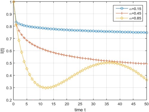
Figure 6. Effects that variation of ρ has on the solution given by (24(24) $\{\begin{array}{l}{I}_1\left(t\right)=I_0,\\ I_n\left(t\right)=I_0{\displaystyle \sum _{k=0}^{n-1}{(-\rho )}^k\frac{{\lambda }^{\frac{k}{2}(k-1)\alpha }{t}^{k\alpha }}{\left(k\alpha \right)!}+\gamma {\displaystyle \sum _{k=1}^{n-1}{(-\rho )}^{k-1}\frac{{\lambda }^{\frac{k}{2}(k-1)\alpha }{t}^{k\alpha }}{\left(k\alpha \right)!},n\in \mathbb{N},n>1.}}\\ I\left(t\right)={\displaystyle \underset{n\to \mathrm{\infty }}{lim}{I}_n\left(t\right).}\end{array}$(24) ).

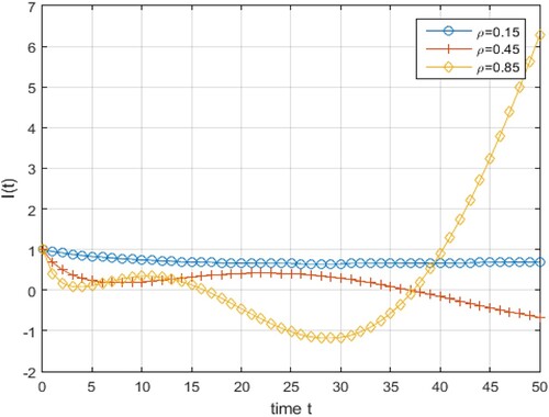
Figure 7. Effects that variation of λ has on the solution given by (24(24) $\{\begin{array}{l}{I}_1\left(t\right)=I_0,\\ I_n\left(t\right)=I_0{\displaystyle \sum _{k=0}^{n-1}{(-\rho )}^k\frac{{\lambda }^{\frac{k}{2}(k-1)\alpha }{t}^{k\alpha }}{\left(k\alpha \right)!}+\gamma {\displaystyle \sum _{k=1}^{n-1}{(-\rho )}^{k-1}\frac{{\lambda }^{\frac{k}{2}(k-1)\alpha }{t}^{k\alpha }}{\left(k\alpha \right)!},n\in \mathbb{N},n>1.}}\\ I\left(t\right)={\displaystyle \underset{n\to \mathrm{\infty }}{lim}{I}_n\left(t\right).}\end{array}$(24) ).

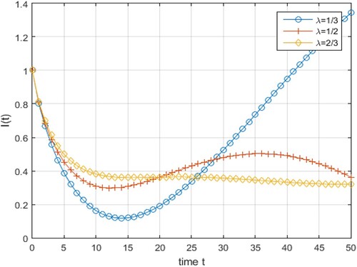
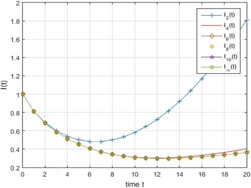
Figure 8. Iterations of the solution given in (24(24) $\{\begin{array}{l}{I}_1\left(t\right)=I_0,\\ I_n\left(t\right)=I_0{\displaystyle \sum _{k=0}^{n-1}{(-\rho )}^k\frac{{\lambda }^{\frac{k}{2}(k-1)\alpha }{t}^{k\alpha }}{\left(k\alpha \right)!}+\gamma {\displaystyle \sum _{k=1}^{n-1}{(-\rho )}^{k-1}\frac{{\lambda }^{\frac{k}{2}(k-1)\alpha }{t}^{k\alpha }}{\left(k\alpha \right)!},n\in \mathbb{N},n>1.}}\\ I\left(t\right)={\displaystyle \underset{n\to \mathrm{\infty }}{lim}{I}_n\left(t\right).}\end{array}$(24) ).

4. Conclusion

This study presented the HSV method for the construction of solutions of fractional differential equations with variable delay that varies with the independent variable. This study shows the potency of the HSV method in obtaining the solutions of differential equations, both with integer-order and fractional derivatives. Solving pantograph-type ODE by using approximate analytical and numerical methods can be considered fairly well developed. Therefore, this study is devoted to pantograph-type equations with Caputo derivatives of fractional variable orders and their applications in Nuclear Physics. The application displays the efficacy of pantograph-type equations with Caputo derivatives of fractional variable orders as an indispensable tool for the modelling of many anomalous phenomena in nature and in the theory of complex systems.

Disclosure statement

The authors declare that they have no known competing financial interests or personal relationships that could have appeared to influence the work reported in this paper.

Availability of data and materials

Data sharing is not applicable to this article as no datasets were generated or analysed during the current study.

Additional information

Funding

MOA acknowledges support from the University of Johannesburg under the GES 4.0 PDRF Award - 223263569. EM acknowledges support from the National Research Foundation of South Africa under grant number 150070.

References

- Mainardi F. Fractional calculus and waves in linear viscoelasticity. London: Imperial College Press; 2010.
- Li C, Deng W. Remarks on fractional derivatives. Appl Math Comput. 2007;187:777–784. doi:10.1016/j.amc.2006.08.163
- Elsgolt's LE, Norkin SB. Introduction to the theory and application of differential equations with deviating arguments. New York (USA): Academic Press; 1973. ISBN: 9780122377501.
- Ockendon JR, Tayler AB. The dynamics of a current collection system for an electric locomotive. Proc R Soc Lond A Math Phys Sci. 1971;322(1551):447–468. doi:10.1098/rspa.1971.0078
- Dehghan M, Shakeri F. The use of the decomposition procedure of adomian for solving a delay differential equation arising in electrodynamics. Phys Scr. 2008;78(6):065004. doi:10.1088/0031-8949/78/06/065004
- Ajello WG, Freedman HI, Wu J. Analysis of a model representing stage-structured population growth with state-dependent time delay. SIAM J Appl Math. 1992;52(3):855–869. doi:10.1137/0152048
- Aibinu MO, Thakur SC, Moyo S. Analyzing population dynamics models via sumudu transform. J Math Comput Sci. 2023;29(03):283–294. doi:10.22436/jmcs
- Mahler K. On a special functional equation. J Lond Math Soc. 1940;s1-15(2):115–123. doi:10.1112/jlms/s1-15.2.115
- Ferguson TS. Lose a dollar or double your fortune. In: Le Cam LM, Neyman J, Scott EL, editors. Proceedings of the 6th Berkeley Symposium on Mathematical Statistics and Probability; Berkeley, CA, USA: University California Press; III, 1972. p. 657–666; ISBN: 9780520021853.
- Robinson RW. Counting labeled acyclic digraphs. In: Harari, F., editor. New Directions in the Theory of Graphs; 1973. New York, NY, USA: Academic Press; p. 239–273. ISBN: 9780123242556.
- Gaver DP. An absorption probability problem. J Math Anal Appl. 1964;9(3):384–393. doi:10.1016/0022-247X(64)90024-1
- Zhang F, Zhang Y. State estimation of neural networks with both time-varying delays and norm-bounded parameter uncertainties via a delay decomposition approach. Commun Nonlinear Sci Numer Simul. 2013;18(12):3517–3529. doi:10.1016/j.cnsns.2013.05.004
- Polyanin AD, Sorokin VG. Nonlinear pantograph-type diffusion PDEs: exact solutions and the principle of analogy. Mathematics. 2021;9(5):511–22. doi:10.3390/math9050511
- Aibinu MO, Thakur SC, Moyo S. Solving delay differential equations via sumudu transform. Int J Nonlinear Anal Appl. 2022;13(2):563–575. doi:10.22075/IJNAA.2021.22682.2402Abstract
- Fox L, Mayers DF, Ockendon JR, et al. On a functional differential equation. IMA J Appl Math. 1971;8(3):271–307. doi:10.1093/imamat/8.3.271
- Bahgat MSM. Approximate analytical solution of the linear and nonlinear multi-pantograph delay differential equations. Phys Scr. 2020;95(5):055219. doi:10.1088/1402-4896/ab6ba2
- Hou C-C, Simos TE, Famelis IT. Neural network solution of pantograph type differential equations. Math Meth Appl Sci. 2020;43(6):3369–3374. doi:10.1002/mma.v43.6
- Alrabaiah H, Ahmad I, Shah K, et al. Qualitative analysis of nonlinear coupled pantograph differential equations of fractional order with integral boundary conditions. Bound Value Probl. 2020;2020(1):138. doi:10.1186/s13661-020-01432-2
- Wang W. Fully-geometric mesh one-leg methods for the generalized pantograph equation: approximating Lyapunov functional and asymptotic contractivity. Appl Numer Math. 2017;117:50–68. doi:10.1016/j.apnum.2017.01.019
- Yang C. Modified Chebyshev collocation method for pantograph-type differential equations. Appl Numer Math. 2018;134:132–144. doi:10.1016/j.apnum.2018.08.002
- Yang C, Lv X. Generalized Jacobi spectral Galerkin method for fractional pantograph differential equation. Math Methods Appl Sci. 2021;44(1):153–165. doi:10.1002/mma.v44.1
- Yel G, Kayhan M, Ciancio A. A new analytical approach to the (1+1)-dimensional conformable fisher equation. Math Model Numer Simul Appl. 2022;2(4):211–220. doi:10.53391/mmnsa.2022.017
- Yavuz M. European option pricing models described by fractional operators with classical and generalized Mittag–Leffler kernels. Numer Methods Partial Differ Equ. 2022;38:434–456. doi:10.1002/num.22645
- Duran S, Durur H, Yavuz M, et al. Discussion of numerical and analytical techniques for the emerging fractional order Murnaghan model in materials science. Opt Quant Electron. 2023;55(6):571. doi: 10.1007/s11082-023-04838-1
- Pak S. Solitary wave solutions for the RLW equation by he's semi inverse method. Int J Nonlinear Sci Numer Simul. 2009;10(4):505–508. doi:10.1515/IJNSNS.2009.10.4.505
- Phang C, Toh YT, Md Nasrudin FS. An operational matrix method based on poly-Bernoulli polynomials for solving fractional delay differential equations. Computation. 2020;8(3):82. doi:10.3390/computation8030082
- Bodkhe DS, Panchal SK. On Sumudu transform of fractional derivatives and its applications to fractional differential equations. Asian J Math Comput Res. 2016;11(1):69–77. https://ikprress.org/index.php/AJOMCOR/article/view/380
- Wu GC, Song TT, Wang SQ. Caputo-Hadamard fractional differential equation on time scales: numerical scheme, asymptotic stability, and chaos. Chaos. 2022;32(9):093143. doi:10.1063/5.0098375
- Song TT, Wu GC, Wei JL. Hadamard fractional calculus on time scales. Fractals. 2022;30(07):2250145. doi:10.1142/S0218348X22501456
- Yavuz M, Sulaiman TA, Usta F, et al. Analysis and numerical computations of the fractional regularized long-wave equation with damping term. Math Methods Appl Sci. 2020;44(9):7538–7555. doi:10.1002/mma.v44.9
- Wei JL, Wu GC, Liu BQ, et al. An optimal neural network design for fractional deep learning of logistic growth, Neural Computing and Applications, 2023, in press, doi:10.1007/s00521-023-08268-8
- Blechschmidt J, Ernst OG. Three ways to solve partial differential equations with neural networks–A review. GAMM-Mitteilungen. 2021;44(2):e202100006. doi:10.1002/gamm.v44.2
- Fang J, Liu C, Simos TE, et al. Neural network solution of single-delay differential equations. Mediterr J Math. 2020;17(1):1–15. doi:10.1007/s00009-019-1452-5
- Hou CC, Simos TE, Famelis IT. Neural network solution of pantograph type differential equations. Math Methods Appl Sci. 2020;43(6):3369–3374. doi:10.1002/mma.v43.6
- Panghal S, Kumar M. Neural network method: delay and system of delay differential equations. Eng Comput. 2022;38(S3):2423–2432. doi:10.1007/s00366-021-01373-z
- Vinodbhai CD, Dubey S. Numerical solution of neutral delay differential equations using orthogonal neural network. Sci Rep. 2023;13(1):3164. doi:10.1038/s41598-023-30127-8
- Colbrook MJ, Antun V, Hansen AC. The difficulty of computing stable and accurate neural networks: on the barriers of deep learning and smale's 18th problem. PNAS. 2022;119(12):e2107151119. doi:10.1073/pnas.2107151119
- Saleh H, Alali E, Ebaid A. Medical applications for the flow of carbon-nanotubes suspended nanofluids in the presence of convective condition using Laplace transform. J Assoc Arab Univ Basic Appl Sci. 2017;24:206–212. doi:10.1016/j.jaubas.2016.12.001
- Khaled S. The exact effects of radiation and joule heating on magnetohydrodynamic Marangoni convection over a flat surface. Therm Sci. 2018;22(1 Part A):63–72. doi:10.2298/TSCI151005050K
- Modanli M, Koksal ME. Laplace transform collocation method for telegraph equations defined by Caputo derivative. Math Model Numer Simul Appl. 2022;2(3):177–186. doi:10.53391/mmnsa.2022.014
- Akgül EK, Akgül A, Yavuz M. New illustrative applications of integral transforms to financial models with different fractional derivatives. Chaos Solitons Fractal. 2021;146:110877. doi:10.1016/j.chaos.2021.110877
- Yavuz M, Sene N. Approximate solutions of the model describing fluid flow using generalized ρ-Laplace transform method and heat balance integral method. Axioms. 2020;9(4):123. doi:10.3390/axioms9040123
- Yavuz M, Abdeljawad T. Nonlinear regularized long-wave models with a new integral transformation applied to the fractional derivative with power and Mittag–Leffler kernel. Adv Differ Equ. 2020;2020(1):367. doi:10.1186/s13662-020-02828-1
- Belgacem FBM, Karaballi A. Sumudu transform fundamental properties investigations and applications. J Appl Math Stoch Anal. 2006;2006:1–23. doi: 10.1155/JAMSA/2006/91083
- Watugala GK. Sumudu transform–a new integral transform to solve differential equations and control engineering problems. Math Eng Ind. 1993;24(1):35–43. doi:10.1080/0020739930240105
- Belgacem FBM, Karaballi AA, Kalla SL. Analytical investigations of the Sumudu transform and applications to integral production equations. Math Prob Eng. 2003;2003(3):103–118. doi:10.1155/S1024123X03207018
- AL-Hussein WRA, Al-Azzawi SN. Approximate solutions for fractional delay differential equations by using Sumudu transform method. In: AIP Conference Proceedings, Vol. 2096, 1, 2019. p. 020007. AIP Publishing LLC.
- Golmankhaneh AK, Tunς C. Sumudu transform in fractal calculus. Appl Math Comput. 2019;350(1):386–401. doi:10.1016/j.amc.2019.01.025
- Alomari AK, Syam MI, Anakira NR, et al. Homotopy Sumudu transform method for solving applications in Physics. Res Phys. 2020;18:103265. doi:10.1016/j.rinp.2020.103265
- Nisar KS, Shaikh A, Rahman G, et al. Solution of fractional kinetic equations involving class of functions and Sumudu transform. Adv Differ Equ. 2020;2020(1):39. doi:10.1186/s13662-020-2513-6
- Roggenkamp PL. The influence of Xenon-135 on reactor operation. Washington Savannah River Company, ID: WSRC-MS-2000-00061, 2000. p. 49–56.
- Zhang W, Zhang D, Wang C, et al. Conceptual design and analysis of a megawatt power level heat pipe cooled space reactor power system. Ann Nucl Energy. 2020;144:107576. doi:10.1016/j.anucene.2020.107576
- Moltot AT, Deresse AT, Edalatpanah SA. Approximate analytical solution to nonlinear delay differential equations by using sumudu iterative method. Adv Math Phys. 2022;2022:1–18. doi:10.1155/2022/2466367
- Sahni M, Parikh M, Sahni R. Sumudu transform for solving ordinary differential equation in a fuzzy environment. J Interdiscip Math. 2021;24(6):1565–1577. doi:10.1080/09720502.2020.1845468
- Nanware JA, Patil NG, Birajdar GA. Applications of Sumudu transform to economic models. Pale J Math. 2022;11(3):636–649. https://pjm.ppu.edu/sites/default/files/papers/PJM_May_%283%292022_636_to_649.pdf
- Wu G. Challenge in the variational iteration method–a new approach to identification of the Lagrange multipliers. J King Saud Univ Sci. 2013;25(2):175–178. doi:10.1016/j.jksus.2012.12.002
- Wu G, Baleanu D. Variational iteration method for fractional calculus–a universal approach by laplace transform. Adv Differ Equ. 2013;2013(1):1–9. doi:10.1186/1687-1847-2013-1
- Tavares D, Almeida R, Torres DFM. Caputo derivatives of fractional variable order: numerical approximations. Commun Nonlinear Sci Numer Simul. 2016;35:69–87. doi:10.1016/j.cnsns.2015.10.027
- Marcillo OE, Maceira M, Chai C, et al. The local seismoacoustic wavefield of a research nuclear reactor and its response to reactor power level. Seismol Res Lett. 2021;92(1):378–387. doi:10.1785/0220200139
- Murray RL. Nuclear energy. 6th ed. Pergamon: Butterworth-Heinemann; 2008. Chapter 6. doi:10.1016/C2013-0-05921-X
- Tayal DC. Nuclear physics. Mumbai: Himalaya Publishing House; 2009. p. 581.
- Stacey WM. Nuclear reactor physics. John Wiley & Sons; 2001. ISBN: 0- 471-39127-1. https://onlinelibrary.wiley.com/doi/book/10.1002/9783527812318
- Lamarsh JR. Introduction to nuclear reactor theory. New York: Addison-Wesley Publishing Company; 2001. p. 501.
- Reuss P. Neutron Physics. EDP Sciences. 2008. ISBN: 978-2759800414.
- Lamarsh JR, Baratta AJ. Introduction to Nuclear Engineering. 3d ed., Prentice-Hall; 2001. ISBN: 0-201-82498-1.
- Lewis EE, Miller WF. Computational Methods of Neutron Transport. American Nuclear Society. 1993. ISBN: 0-894-48452-4.
- WNA. World Nuclear Association (WNA) Image Library. https://www.world-nuclear.org/gallery/reactor-diagrams/pressurized-water-reactor.aspx Accessed 2023 Mar 30.