
 ?Mathematical formulae have been encoded as MathML and are displayed in this HTML version using MathJax in order to improve their display. Uncheck the box to turn MathJax off. This feature requires Javascript. Click on a formula to zoom.
ABSTRACT
The type of symmetry exhibited by a travelling wave can have important implications for its behaviour and properties, such as its polarization, dispersion, and interactions with other waves or boundaries. The fractional differential Duffing problem refers to the mathematical modelling of nonlinear, damped oscillations of a system with fractional derivatives. It is a generalization of the classical Duffing equation, which describes the behaviour of a nonlinear, damped oscillator (the equation becomes symmetric under time-reversal). The fractional derivatives allow for a more accurate description of the system's memory and hereditary properties. The solution of the fractional Duffing equation can provide insight into the complex dynamic behaviour of various physical, biological, and engineering systems. We are concerned with studying a new differential Duffing fractional problem. It involves some sequential Caputo derivatives with an infinite series of Riemann–Liouville integrals and some other functions. We begin by proving a first existence and uniqueness result, then we discuss two types of stability for the obtained uniqueness result. An illustrative examples is given to show the applicability of the result. We are also concerned with applying the Tanh method to obtain new classes of travelling wave solutions for three important classes of (Khalil) fractional conformable problems; the generalized equation of Duffing, the Landau–Ginzburg–Higgs equation and the Sine–Gordon one. Some numerical simulations are plotted and a conclusion is given at the end.
1. Introduction
The Duffing phenomenon is named after Georg Duffing, and refers to the nonlinear behaviour of a mechanical system, such as a spring-mass system, that experiences both damping and a periodic forcing. The nonlinearity results in the occurrence of a variety of dynamic behaviours, including limit cycles and chaos, which are not present in linear systems. The Duffing equation is widely used as a model to study nonlinear vibrations and chaos in various fields, including mechanical engineering, physics, and control systems. The Duffing equation is a nonlinear, second-order ordinary differential equation that describes the dynamics of a system subjected to a periodic driving force and a nonlinear restoring force (see [Citation1–5]).
Traveling waves can exhibit different types of symmetry, depending on the characteristics of the wave and the medium through which it travels. Here are some examples of symmetry in travelling waves:
Reflection symmetry: A wave has reflection symmetry if it looks the same when reflected in a line or plane. For example, a sinusoidal wave that travels along a string has reflection symmetry because it looks the same when reflected in the string.
Translational symmetry: A wave has translational symmetry if it looks the same after it has been shifted by a fixed distance. For example, a wave that travels along an infinitely long string has translational symmetry because it looks the same at any point along the string.
Rotational symmetry: A wave has rotational symmetry if it looks the same after it has been rotated around a fixed point. For example, a circular wave that travels outward from a point source has rotational symmetry because it looks the same when viewed from any angle around the source. Time-reversal symmetry: A wave has time-reversal symmetry if it looks the same when time is reversed. For example, an electromagnetic wave that travels through free space has time-reversal symmetry because it looks the same whether it is moving forward or backward in time. In addition, the Duffing equation is symmetric under the transformation
, which is known as the parity transformation. This means that if the displacement x of the oscillator is replaced with its negative, the equation remains unchanged.
Fractional Differential Equations (FDEs) are mathematical equations that involve derivatives of non-integer order. Unlike traditional differential equations, which involve integer order derivatives, FDEs allow for the modelling of complex physical processes that exhibit memory and hereditary properties. FDEs are widely used in various fields including physics, engineering, finance, and biology to study problems such as anomalous diffusion, control theory, and viscoelasticity. The solution methods for FDEs include the Laplace transform, the Fourier transform, numerical techniques, and variational methods. The term ‘conformable derivative’ refers to a type of derivative that can be used in mathematical models to describe the rate of change of a function. It is similar to a traditional derivative, but is designed to handle functions with non-uniform scales. The concept is used in various branches of mathematics, including fractional calculus and mathematical finance [Citation6].
The fractional Duffing phenomenon refers to the nonlinear behaviour of a mechanical system that experiences both damping and a periodic forcing, described by a fractional differential equation. Fractional differential equations are a generalization of the classical differential equations and can model complex dynamic behaviours, including memory and long-range dependence, which are not possible to capture using classical differential equations. The fractional Duffing equation is used to study nonlinear vibrations and chaos in systems that exhibit fractional dynamic behaviour, such as in viscoelastic materials, complex networks, and biological systems. The fractional Duffing equation has been found to exhibit a wider range of dynamic behaviours compared to the classical Duffing equation, including multistability, bifurcations, and chaotic attractors.
The oscillator phenomena have several applications in science and engineering. One of such oscillators is the Duffing phenomenon [Citation7]. The equation of Duffing is a nonlinear problem [Citation8,Citation9]. It has been used successfully for modelling a variety of physical and chemical processes, reinforcing springs, beam buckling, nonlinear electronic circuits,…
The forced form of Duffing equation is:
where
is the displacement at time,
is the velocity, and
is the acceleration. The numbers p, q, s, r and ω are some given constants.
Up to now, many methods used for solving the above ‘forced’ equation and other nonlinear differential equations are developed, for example the first integral method [Citation10], the exp-function method [Citation11,Citation12], the (G'/G) method [Citation13], the Jacobi method [Citation14], and the tanh method [Citation15,Citation16]. The tanh method seems to be one of the important algebraic methods serving to obtain solutions and explicit travelling waves for nonlinear differential problems, see for instance [Citation15,Citation17,Citation18].
On the other hand, fractional differential problems have attracted attention of researchers for several times; they have been applied in physics, chemistry, biology to model many real word phenomena, see [Citation19–23].
In this sense, in [Citation24], by using Riemann–Liouville derivatives, V.A. Kim has considered the following problem of type Duffing:
Also in [Citation25], Y. Gouari et al. have investigated the following problem with Duffing type that involves sequential derivatives:
Very recently in [Citation12], M. Rakah et al. have taken into account the study of the following problem:
The existence of one solution has been treated by the authors.
In the work [Citation26], the authors have looked for the investigation of the following sequential VdP Duffing equation:
They have studied the problem by using Caputo Hadamard approach. They have established new conditions for studying the solutions for the problem. The stability has also been discussed in their paper.
The aim of the first part of the present work is to study the following generalized fractional differential problem:
(1)
(1)
For (Equation1
(1)
(1) ), we take J the interval
also, we consider that
, and each derivative of the problem is of Caputo,
is the Riemann–Liouville integral, the functions f and g are supposed to be defined from
to
, also
are continuous, and
are defined and continuous over
,
are defined over J,
, the constants
are some reals.
We begin by proving an integral representation for our problem. Then, an existence and uniqueness result is established. Also, we study the stability of the unique ‘proved’ solution. An illustrative example is then discussed in details.
In the second part of the present work, we will use the method of tanh to obtain new travelling waves for three important problems of type:
(2)
(2)
where
are fractional derivatives of conformable type [Citation27] (for more extended operator, one can see [Citation28,Citation29]), with
and a, b, s, d are some real constants.
2. Background
In this Background second section, we have to present to the reader some definitions of fractional calculus theory, see [Citation30,Citation31].
Definition 2.1
We consider and
. Then the derivative of Caputo with order α for v is:
such that
the integer part of the parameter α.
Definition 2.2
The Riemann–Liouville integral of order for any function
is given by
Lemma 2.3
The solution of the generalized fractional equation ,
, has the form:
taking into account that
.
Lemma 2.4
If α and β are two positive parameters, then we have
Lemma 2.5
Let G be a Banach space and is an application that is contractible. Then, Z has exactly one fixed point in G.
Let us now present then prove another lemma.
Lemma 2.6
We consider K and
in
. Then, the BVP
(3)
(3)
is equivalent to the following representation:
(4)
(4)
such that
Proof.
It is easy to see that the equation
permits us to write
(5)
(5)
Using some of the above initial conditions, we get:
By substitution, we get
On the other hand, we have
By using the fact that
, we observe that:
Inserting the values of
in (Equation5
(5)
(5) ), we end the proof.
3. Main results
3.1. Part 1: uniqueness of solutions and stability
Let us consider space
with the norm is defined by
where,
In addition, we define
by:
(6)
(6)
where
Now, we have to consider the three hypotheses:
| (F1): | The given functions of (Equation1 | ||||
| (F2): | There exist non-negative continuous functions | ||||
| (F3): | Suppose that | ||||
Now, we consider the quantities:
and
3.1.1. A unique solution
We present the first result as follows:
Theorem 3.1
We consider that , and
are verified. Also, we suppose
Thus, (Equation1
(1)
(1) ) has a unique solution defined on J.
Proof.
We try to prove the contraction of W.
We take any , so we immediately get
(7)
(7)
We have also
(8)
(8)
With the same arguments as before, we have
(9)
(9)
From (Equation7
(7)
(7) ) and (Equation9
(9)
(9) ), we get
We see that W a contraction application. Therefore, we prove the uniqueness of fixed point for W, which is the solution of (Equation1
(1)
(1) ).
Example:
As an example, we can take the special problem:
(10)
(10)
where,
Theorem 3.1 allows the reader to confirm for the above example, we have exactly one solution.
3.1.2. Stability of the unique solution
We introduce the following definitions
Definition 3.2
We say that (Equation1(1)
(1) ) is stable in the sense of Ulam Hyers if there is a
, such that for each positive ϵ and for an arbitrary solution
of
(11)
(11)
we can obtain a solution
of (Equation1
(1)
(1) ), with
Definition 3.3
We say that (Equation1(1)
(1) ) is stabel in the generalised sens of Ulam Hyers if we can find a function
;
; that verifies for any positive ϵ, and for each solution
of (Equation11
(11)
(11) ), there is
solution of (Equation1
(1)
(1) ); with
We pass to consider the following main theorem.
Theorem 3.4
Suppose all the hypotheses of 3.1 are valid. Then, (Equation1(1)
(1) ) is stable in Ulam Hyers sense.
Proof.
We take a solution of (Equation11
(11)
(11) ). Therefore, Theorem 3.1 guarantees the existence of a unique solution
for (Equation1
(1)
(1) ).
Using (Equation11(11)
(11) ), we observe that
(12)
(12)
Using (Equation11
(11)
(11) ) and (Equation12
(12)
(12) ), we get
Therefore,
Thus,
On the other hand, we have
Consequently,
In consequence, (Equation1
(1)
(1) ) is stable in the sense of Ulam Hyers.
Remark 3.5
By considering the case where , we can obtain the stability in the generalised sense for (Equation1
(1)
(1) ).
3.2. Part 2: new travelling wave solutions by tanh method
We are interested in applying the method of Tanh to solve some fractional conformable problems of type:
where
are the conformable fractional derivative, with α and β are in
and
.
Note that when the above equation can be transformed into the following type of Duffing equation [Citation32]:
(13)
(13)
3.2.1. Conformable derivatives
We need to introduce the following preliminaries (see [Citation27,Citation33,Citation34])
Definition 3.6
Taking the function f defined over . The conformable derivative with a fractional order α in
is:
Definition 3.7
The conformable integral of any function defined over the infinite interval of order α is given by
Based on the above definitions, we have:
and
3.2.2. Method of tanh
We consider the equation
(14)
(14)
where
is the fractional conformable derivative of u of order
. Introducing the new wave variable
(15)
(15)
so, (Equation15
(15)
(15) ) can be transformed to the equation:
(16)
(16)
We then put
(17)
(17)
So, we have
(18)
(18)
Now, we consider
(19)
(19)
The parameter m is to be obtained.
3.2.3. Applications
Example 3.1
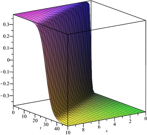
We take the Landau–Ginzburg–Higgs equation [Citation35] (Figure ):
(20)
(20)
Using (Equation15
(15)
(15) ), we change (Equation20
(20)
(20) ) into the following nonlinear ODE
(21)
(21)
Substituting (Equation18
(18)
(18) ) and (Equation19
(19)
(19) ) into (Equation21
(21)
(21) ), we can get
(22)
(22)
We ‘balance’
with
to obtain m = 1.
Figure 1. 3D-plot of case1-travelling wave solution of (Equation20(20)
(20) ) with
and
.
So, we have
(23)
(23)
Substituting (Equation23
(23)
(23) ) into (Equation22
(22)
(22) ), we can get
(24)
(24)
from which we obtain
Solving the above system, we get the following new travelling waves:
Case 1:
(25)
(25)
Case 2:
(26)
(26)
Example 3.2
We take the example of Sine–Gordon equation [Citation32,Citation36] (Figure ):
(27)
(27)
We have
(28)
(28)
Substituting (Equation18
(18)
(18) ) and (Equation19
(19)
(19) ) into (Equation28
(28)
(28) ), we can get
(29)
(29)
On the other hand, we have
(30)
(30)
Substituting (Equation30
(30)
(30) ) into (Equation29
(29)
(29) ), yields
(31)
(31)
Then, we have the algebraic system:
We solve the above system and hence, we have the following cases giving travelling waves:
Figure 2. 3D plot of case1-travelling wave solution of (Equation27(27)
(27) ) with
and
.
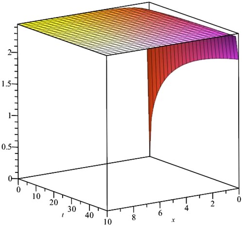
Case 1:
(32)
(32)
Case 2:
(33)
(33)
Example 3.3
Now, we would like to find the travelling waves for the problem [Citation32,Citation36] (Figure ):
(34)
(34)
It can be transformed into the equation
(35)
(35)
Substituting (Equation18
(18)
(18) ) and (Equation19
(19)
(19) ) into (Equation35
(35)
(35) ), we can get
(36)
(36)
So, we have
(37)
(37)
Substituting (Equation37
(37)
(37) ) into (Equation36
(36)
(36) ), we can get
(38)
(38)
The algebraic system allows us to obtain the following travelling wave solutions of (Equation34
(34)
(34) ):
Figure 3. 3D plot of travelling wave solution for case1 of (Equation34(34)
(34) ) with:
and
.
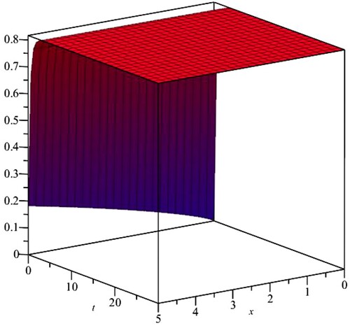
Case 1:
(39)
(39)
Case 2:
(40)
(40)
4. Conclusion
We have first proposed a new sequential nonlinear differential problem with nonlocal integral conditions that involves convergent series in its right-hand sides by means of fractional derivatives (Equation1(1)
(1) ). Our problem involves n sequential derivatives of Caputo type. Then, we have used Banach contraction principle to discuss a result on the existence of a unique solution. An example has been presented. A stability result has also been discussed. In the second part, we have used Khalil approach and applied the method of tanh to find new travelling waves for some interesting fractional differential equations that are similar to (Equation2
(2)
(2) ); we cite Duffing, Landau–Ginzburg–Higgs and CTF Sine-Gordon fractional conformable equations. Some
graphs on the obtained travelling waves are plotted in different cases.
Disclosure statement
No potential conflict of interest was reported by the author(s).
Data availability statement
No data were used to support this study.
References
- Abbas MI, Alessandra MR. Nonlinear fractional differential inclusions with non-singular Mittag-Leffler kernel. AIMS Math. 2022;7(11):20328–20340. doi: 10.3934/math.20221113
- Guariglia E. Fractional calculus, zeta functions and Shannon entropy. Open Math. 2021;19(1):87–100. doi: 10.1515/math-2021-0010
- Guariglia E. Riemann zeta fractional derivative-functional equation and link with primes. Adv Differ Equ. 2019;1:1–15. doi: 10.1186/s13662-019-2202-5
- Li C, Xuanhung D, Peng G. Fractional derivatives in complex planes. Nonlinear Anal Theory Methods Appl. 2009;71(5–6):1857–1869. doi: 10.1016/j.na.2009.01.021
- Ragusa MA. Commutators of fractional integral operators on vanishing-Morrey spaces. J Glob Optim. 2008;40:361–368. doi: 10.1007/s10898-007-9176-7
- Atangana A, Akgul A, Altaf Khan M, et al. Conformable derivative: a derivative associated to the Riemann-Stieltjes integral. Progr Fract Differ Appl. 2022;8(2):321–348. doi: 10.18576/pfda
- Duffing G. Erzwungene schwingungen bei veränderlicher eigenfrequenz und ihre technische bedeutung. Braunschweig, Germany: Vieweg Sohn; 1918. (Sammlung Vieweg).
- Abolfazl J, Hadi F. The application of duffing oscillator in weak signal detection. ECTI Trans Electr Eng Electron Commun. 2011; 9(1):1–6. doi: 10.37936/ecti-eec.201191.172249
- Sunday J. The duffing oscillator: applications and computational simulations. Asian Res J Math. 2017. doi: 10.9734/ARJOM/2017/31199
- Lu B. The first integral method for some time fractional differential equations. J Math Anal Appl. 2012;395:684–693. doi: 10.1016/j.jmaa.2012.05.066
- He JH. Exp-function method for fractional differential equations. Int J Nonlinear Sci Numer Simul. 2013;14(6):363–366. doi: 10.1515/ijnsns-2011-0132
- Rakah M, Anber A, Dahmani Z, et al. An analytic and numerical study for two classes of differential equation of fractional order involving Caputo and Khalil derivative. An Stiint Univ Al I Cuza Iasi Mat (NS). Accepted 2022.
- Zheng B. (G'/G)-Expansion method for solving fractional partial differential equations in the theory of mathematical physics. Commun Theor Phys. 2012;58:623–630. doi: 10.1088/0253-6102/58/5/02
- Lu D, Shi Q. New Jacobi elliptic functions solutions for the combined KdV-MKdV equation. Int J Nonlinear Sci. 2010;10(3):320–325.
- Malfliet W. Solitary wave solutions of nonlinear wave equations. Am J Phys. 1992;60(7):650–654. doi: 10.1119/1.17120
- Rakah M, Dahmani Z, Senouci A. New uniqueness results for fractional differential equations with a caputo and khalil derivatives. Appl Math Inf Sci. 2022;16(6):943–952. doi: 10.18576/amis
- Malfliet W. The tanh method: I. Exact solutions of nonlinear evolution and wave equations. Phys Scr. 1996;54:563–568. doi: 10.1088/0031-8949/54/6/003
- Wazwaz AM. The tanh method for compact and non compact solutions for variants of the KdV-Burger equations. Phys D Nonlinear Phenom. 2006;213:147–151. doi: 10.1016/j.physd.2005.09.018
- Bachar I, Eltayeb H. Existence and uniqueness results for fractional Navier boundary value problems. Adv Differ Equ. 2020;609. doi: 10.1186/s13662-020-03071-4
- Dahmani Z, Abdellaoui MA, Houas M. Coupled systems of fractional integro-differential equations involving several functions. Theory Appl Math Comput Sci. 2015;5(1):53–61.
- Dahmani Z, Bahous Y, Bekkouche Z. A two parameter singular fractional differential equations of Lane emden type. Turkish J Inequal. 2019;3(1):35–53.
- Gouari Y, Dahmani Z, Farooq SE, et al. Fractional singular differential systems of lane emden type: Existence and uniqueness of solutions. Axioms. 2020;9(3):1–18. doi: 10.3390/axioms9030095
- Gouari Y, Dahmani Z, Belhamiti M, et al. Uniqueness of solutions, stability and simulations for a differential problem involving convergent series and time variable singularities. Rocky Mt J Math. 2022. doi: 10.22541/au.163673427.78470853/v1
- Kim VA. Duffing oscillator with external harmonic action and variable fractional Riemann-Liouville derivative characterizing viscous friction. Bull KRASEC Phys Math Sci. 2016;13:46–49. doi: 10.18454/2313-0156-2016-13-2-46-49
- Gouari Y, Dahmani Z, Jebril I. Application of fractional calculus on a new differential problem of duffing type. Adv Math Sci J. 2020;9:10989–11002. doi: 10.37418/amsj
- Abdenebi A, Dahmani Z. New van der Pol-Duffing jerk fractional differential oscillator of sequential type. Mathematics. 2022;10:3546. doi: 10.3390/math10193546
- Khalil R, Al Horani M, Yousef A, et al. A new definition of fractional derivative. J Comput Appl Math. 2014;264:65–70. doi: 10.1016/j.cam.2014.01.002
- Ibrahim RW. K-symbol fractional order discrete-time models of Lozi system. J Differ Equ Appl. 2022;12:1–20 doi: 10.1080/10236198.2022.2158736
- Al-Shamasneh A, Ibrahim RW. Image denoising based on quantum calculus of local fractional entropy. Symmetry. 2023;15(2):396. doi: 10.3390/sym15020396
- Kilbas AA, Srivastava HM, Trujillo JJ. Theory and applications of fractional differential equations. Amsterdam: Elsevier B.V; 2006.
- Miller KS, Ross B. An introduction to the fractional calculus and fractional differential equations. New York: Wiley; 1993.
- Tie-cheng X, Hong-qing Z, Zhen-ya Y. New explicit and exact travelling wave solutions for a class of nonlinear evolution equations. Appl Math Mech. 2001;22:788–793. doi: 10.1007/BF02438222
- Abdeljawad T. On conformable fractional calculus. J Comput Appl Math. 2015;279:57–66. doi: 10.1016/j.cam.2014.10.016
- Dahmani Z, Anber A, Gouari A, et al. Extension of a method for solving nonlinear evolution equations via conformable fractional approach. In: International Conference on Information Technology; IEEE, Amman, Jordan. 2021; p. 38–42.
- Hu WP, Deng ZC, Han SM, et al. Multi-symplectic Runge-Kutta method for Landau Ginzburg-Higgs equation. Appl Math Mech. 2009;30(8):1027–1034. doi: 10.1007/s10483-009-0809-x
- Xie F, Gao X. Exact travelling wave solutions for a class of nonlinear partial differential equations. Chaos Soliton Fract. 2004;19:1113–1117. doi: 10.1016/S0960-0779(03)00298-4