Exploring the role of fractal-fractional operators in mathematical modelling of corruption

Abstract

In the proposed manuscript, we present a novel mathematical model for analysing the persistence of corruption in human communities, based on fractal-fractional concepts and the Mittag-Leffler kernel law. Corruption is considered analogous to a disease that can spread and influence others who are free from corruption. Our model evaluates the equilibrium points of corruption and tests their stability using the corruption reproduction number. We also apply the fixed point theory concept to check for the existence and uniqueness of a solution, in the context of a fractional fractal operator. Solution stability is verified using the perturbed Ulam Hyers technique, and an approximate solution is obtained through the use of Lagrangian polynomials. To test the validity of our model, we simulate all compartments at different fractional orders and time durations, providing additional insights into the dynamics of corruption beyond natural orders.

Keywords:

• Corruption model
• sensitivity analysis
• positive solution
• Mittag-Leffler kernel law
• qualitative analysis
• ulam hyers stability
• approximate solution

Mathematics Subject Classifications:

• 34D20
• 47-04
• 47-08
• 47J05

1. Introduction

In the last few decades, corruption has received increasing attention in the literature and debates on development and political economics. Corruption is generally defined as dishonest or criminal behaviour carried out by individuals or organizations in positions of authority, in order to gain illegal benefits or use their power for personal gain. Such behaviour may include bribery, influence peddling, embezzlement, and other actions that may be permitted in some countries [1,2]. Political corruption refers to the abuse of power by government officials, including politicians, for their personal benefit. Unfortunately, such criminal behaviour is pervasive and occurs with varying degrees and proportions in almost all countries around the world, becoming a significant sociological issue. Corruption is a failure of ethics, and countries invest substantial resources in efforts to combat it. The term ‘anti-corruption’ is a broad umbrella term that encompasses various tactics employed to prevent and combat corruption [3].

Corruption has been a significant barrier to achieving sustainable development goals in developing countries, and it remains a major obstacle for individuals and nations with low standards, showing a strong correlation with poverty. Its effects are not limited to the social and political sectors, as it also has far-reaching impacts on the economy, culture, psychology, and the environment. Corruption has been present throughout history and is not a modern issue. Ancient Indian philosopher Chanakya believed that corruption is an inherent part of the human brain, and avoiding it is as challenging as resisting the allure of honey. Corruption is a complex and pervasive problem, taking on many forms, from blatant to insidious. According to English historian Edward Gibbon, corruption is the most accurate indicator of constitutional liberty. German philosopher Arthur Schopenhauer recognized that even academics and philosophers are susceptible to the same causes of corruption as the cultures in which they live. He drew a distinction between the sincere philosopher, whose sole aim is to learn the truth and bear witness to it, and the dishonest ‘university,’ whose true goal is to gain recognition, earn an honest income, and enjoy a certain status in the public eye [4]. Corruption undermines public confidence in the socio-political system and fosters dishonest practices, immorality, illegality, injustice, subjectivity, inefficiency, and insincerity, all of which corrode the moral foundations of society and undermine the principles of public service.

The use of modelling and optimization techniques can aid in comprehending the dynamics of corruption transmission and devising efficient strategies to address it. Researchers such as Abdulrahman, Brianzoni, and MAU have studied the epidemiological modelling of corruption [5–7]. Alvaro devised a system for evaluating the dynamics of corruption by computing the average rate of corruption spread in society and the equilibrium points at which corruption is either absent or widespread [8]. The SIR mathematical model for dynamic corruption was investigated by Athithan and colleagues, who incorporated optimal control aspects by modifying the equations [9]. Lemecha developed a corruption prevention model that proved the possibility of perfect corruption prevention if the rates of dismissal and corruption are identical [10]. Despite its relevance to development and political economics, corruption has been the subject of relatively few scientific publications.

2. Model formulation

The total population of society, denoted by $\mathcal{N}$, is divided into six compartments: Susceptible individuals ($I_{\mathcal{S}}$), Risky individuals ($I_{\mathcal{R}}$), Corrupt individuals ($I_{\mathcal{C}}$), Punished individuals ($I_{\mathcal{P}}$), Transformed individuals ($I_{\mathcal{T}}$), and Immune individuals ($I_{\mathcal{I}}$).

Motivated by the above studies, we propose a mathematical model to study the transmission and optimal control strategies for corruption behaviour in society [11]. Specifically, we consider a corruption transmission model. (1) $\{\begin{array}{l}{\dot{I}}_{\mathcal{S}}\left(t\right)=\nu \mathrm{\Psi }-{\lambda }_{I_{\mathcal{S}}}{I}_{\mathcal{S}}\left(t\right)I_{\mathcal{C}}\left(t\right)+\theta {\psi }_{I_{\mathcal{T}}}{I}_{\mathcal{T}}\left(t\right)-\gamma I_{\mathcal{S}}\left(t\right),\\ {\dot{I}}_{\mathcal{R}}\left(t\right)={\lambda }_{I_{\mathcal{S}}}{I}_{\mathcal{S}}\left(t\right)I_{\mathcal{C}}\left(t\right)+{\lambda }_{I_{\mathcal{R}}}{I}_{\mathcal{R}}\left(t\right)I_{\mathcal{C}}\left(t\right)-({\psi }_{I_{\mathcal{R}}}+\gamma )I_{\mathcal{R}}\left(t\right),\\ {\dot{I}}_{\mathcal{C}}\left(t\right)=\text{β}{\psi }_{I_{\mathcal{R}}}{I}_{\mathcal{R}}\left(t\right)-{\lambda }_{I_{\mathcal{R}}}{I}_{\mathcal{R}}\left(t\right)I_{\mathcal{C}}\left(t\right)-({\psi }_{I_{\mathcal{C}}}+\gamma )I_{\mathcal{C}}\left(t\right),\\ {\dot{I}}_{\mathcal{P}}\left(t\right)={\psi }_{I_{\mathcal{C}}}{I}_{\mathcal{C}}\left(t\right)-({\psi }_{I_{\mathcal{P}}}+\gamma )I_{\mathcal{P}}\left(t\right),\\ {\dot{I}}_{\mathcal{T}}\left(t\right)={\psi }_{I_{\mathcal{P}}}{I}_{\mathcal{P}}\left(t\right)+(1-\lambda ){\psi }_{I_{\mathcal{R}}}{I}_{\mathcal{R}}\left(t\right)-(\gamma +{\psi }_{I_{\mathcal{T}}})I_{\mathcal{T}}\left(t\right),\\ {\dot{I}}_{\mathcal{I}}\left(t\right)=(1-\nu )\mathrm{\Psi }+(1-\theta ){\psi }_{I_{\mathcal{T}}}{I}_{\mathcal{T}}\left(t\right)-\gamma I_{\mathcal{I}}\left(t\right),\end{array}$(1) with initial conditions (2) $\{\begin{array}{l}{I}_{\mathcal{S}}\ge 0,I_{\mathcal{R}}\ge 0,I_{\mathcal{C}}\ge 0,I_{\mathcal{P}}\ge 0,I_{\mathcal{T}}\ge 0,I_{\mathcal{I}}\ge 0.\end{array}$(2) The parameters used in model (1(1) $\{\begin{array}{l}{\dot{I}}_{\mathcal{S}}\left(t\right)=\nu \mathrm{\Psi }-{\lambda }_{I_{\mathcal{S}}}{I}_{\mathcal{S}}\left(t\right)I_{\mathcal{C}}\left(t\right)+\theta {\psi }_{I_{\mathcal{T}}}{I}_{\mathcal{T}}\left(t\right)-\gamma I_{\mathcal{S}}\left(t\right),\\ {\dot{I}}_{\mathcal{R}}\left(t\right)={\lambda }_{I_{\mathcal{S}}}{I}_{\mathcal{S}}\left(t\right)I_{\mathcal{C}}\left(t\right)+{\lambda }_{I_{\mathcal{R}}}{I}_{\mathcal{R}}\left(t\right)I_{\mathcal{C}}\left(t\right)-({\psi }_{I_{\mathcal{R}}}+\gamma )I_{\mathcal{R}}\left(t\right),\\ {\dot{I}}_{\mathcal{C}}\left(t\right)=\text{β}{\psi }_{I_{\mathcal{R}}}{I}_{\mathcal{R}}\left(t\right)-{\lambda }_{I_{\mathcal{R}}}{I}_{\mathcal{R}}\left(t\right)I_{\mathcal{C}}\left(t\right)-({\psi }_{I_{\mathcal{C}}}+\gamma )I_{\mathcal{C}}\left(t\right),\\ {\dot{I}}_{\mathcal{P}}\left(t\right)={\psi }_{I_{\mathcal{C}}}{I}_{\mathcal{C}}\left(t\right)-({\psi }_{I_{\mathcal{P}}}+\gamma )I_{\mathcal{P}}\left(t\right),\\ {\dot{I}}_{\mathcal{T}}\left(t\right)={\psi }_{I_{\mathcal{P}}}{I}_{\mathcal{P}}\left(t\right)+(1-\lambda ){\psi }_{I_{\mathcal{R}}}{I}_{\mathcal{R}}\left(t\right)-(\gamma +{\psi }_{I_{\mathcal{T}}})I_{\mathcal{T}}\left(t\right),\\ {\dot{I}}_{\mathcal{I}}\left(t\right)=(1-\nu )\mathrm{\Psi }+(1-\theta ){\psi }_{I_{\mathcal{T}}}{I}_{\mathcal{T}}\left(t\right)-\gamma I_{\mathcal{I}}\left(t\right),\end{array}$(1) ) are as follows: ν represents the individuals who have not recruited immunity, Ψ represents the population growth through recruitment, ${\lambda }_{I_{\mathcal{S}}}$ is the probability of corruption transfer per contact, θ represents the rate of individuals transferred to the susceptible class, γ represents the natural death rate, ${\xi }_{I_{\mathcal{T}}}$ is the outflow of the proportion of people undergoing transformation, ${\lambda }_{I_{\mathcal{R}}}$ is the rate of corruption class to risk cases, ${\psi }_{I_{\mathcal{R}}}$ is the proportionality of the outflow of the risk population, β is the rate of the risk class switching to the corruption cases, ${\psi }_{I_{\mathcal{C}}}$ is the rate of corrupt individuals entering the punished class, and ${\xi }_{I_{\mathcal{P}}}$ represents the rate of corrupt individuals entering the transferred class.

The generalized analysis of modern calculus has garnered significant interest from mathematics and physics scholars over the last few decades, due to its numerous applications in the fields of physics and other material sciences for simulating a vast number of real-world phenomena in physical, chaos theory, and biological sciences [12,13]. In modern calculus mathematical models, the power of the derivative and integration can be chosen as any integer value or any value lying between integers. Fractional calculus employs many concepts used for different fractional operators that are employed in a wide range of applied science domains [14–16]. Fractional calculus has been successfully used by researchers in a variety of fields, including quantum physics, fluid dynamics, electromagnetic theory, viscoelasticity, and signal processing. To comprehend these systems' behaviour and draw meaningful conclusions from experimental data, fractional differential equations and fractional integral operators are useful tools [17–21]. In particular, in the area of mathematical physics, several scientists have successfully employed fractional calculus to describe a broad variety of phenomena in various domains. A robust mathematical foundation for analysing systems and processes that display non-local or non-integer order behaviour is provided by fractional calculus [22–25]. Fractional calculus also provides a greater comprehension of fundamental physical concepts and can result in fresh perceptions and discoveries. It has shown to be especially helpful in the study of anomalous diffusion, power-law correlations, and self-similar patterns, all of which are seen in a variety of natural and artificial systems. Researchers have applied useful operators to solve linear and nonlinear complex problems, demonstrating the validity of the operators used [26–29]. In modern calculus, the power of the derivative and integration can take on any integer value or any value between integers, thereby generalizing the concept of classical calculus [30–32]. Similarly, if the equation being considered has a fractal dimension, then the fractal derivative becomes unity $\lambda t^{\lambda -1}$. Atangana presented the concept of a fractal-fractional (FF) operator and examined the relationship between fractal and fractional calculus [33]. Fractal-fractional calculus is a new field that has emerged from the combination of fractal and fractional notions. By using this derivative, complex problems can be solved with both operators simultaneously. If we take the fractional order of the derivative to be one, we obtain an ordinary system, and by taking a non-integer order, we have a fractional system. This combined operators approach is significant for studying real-world problems that have a fractal dimension and require the use of fractional derivatives alone. Thus, these operators offer new opportunities for the analysis of complex phenomena [33–37].

The system (1(1) $\{\begin{array}{l}{\dot{I}}_{\mathcal{S}}\left(t\right)=\nu \mathrm{\Psi }-{\lambda }_{I_{\mathcal{S}}}{I}_{\mathcal{S}}\left(t\right)I_{\mathcal{C}}\left(t\right)+\theta {\psi }_{I_{\mathcal{T}}}{I}_{\mathcal{T}}\left(t\right)-\gamma I_{\mathcal{S}}\left(t\right),\\ {\dot{I}}_{\mathcal{R}}\left(t\right)={\lambda }_{I_{\mathcal{S}}}{I}_{\mathcal{S}}\left(t\right)I_{\mathcal{C}}\left(t\right)+{\lambda }_{I_{\mathcal{R}}}{I}_{\mathcal{R}}\left(t\right)I_{\mathcal{C}}\left(t\right)-({\psi }_{I_{\mathcal{R}}}+\gamma )I_{\mathcal{R}}\left(t\right),\\ {\dot{I}}_{\mathcal{C}}\left(t\right)=\text{β}{\psi }_{I_{\mathcal{R}}}{I}_{\mathcal{R}}\left(t\right)-{\lambda }_{I_{\mathcal{R}}}{I}_{\mathcal{R}}\left(t\right)I_{\mathcal{C}}\left(t\right)-({\psi }_{I_{\mathcal{C}}}+\gamma )I_{\mathcal{C}}\left(t\right),\\ {\dot{I}}_{\mathcal{P}}\left(t\right)={\psi }_{I_{\mathcal{C}}}{I}_{\mathcal{C}}\left(t\right)-({\psi }_{I_{\mathcal{P}}}+\gamma )I_{\mathcal{P}}\left(t\right),\\ {\dot{I}}_{\mathcal{T}}\left(t\right)={\psi }_{I_{\mathcal{P}}}{I}_{\mathcal{P}}\left(t\right)+(1-\lambda ){\psi }_{I_{\mathcal{R}}}{I}_{\mathcal{R}}\left(t\right)-(\gamma +{\psi }_{I_{\mathcal{T}}})I_{\mathcal{T}}\left(t\right),\\ {\dot{I}}_{\mathcal{I}}\left(t\right)=(1-\nu )\mathrm{\Psi }+(1-\theta ){\psi }_{I_{\mathcal{T}}}{I}_{\mathcal{T}}\left(t\right)-\gamma I_{\mathcal{I}}\left(t\right),\end{array}$(1) ), mentioned earlier, can be described by including a fractional order $0<\rho \le 1$ and a fractal dimension $0<\kappa \le 1$. The resulting system is given below: (3) $\begin{array}{rl}{}_0^{FFABC}{D}_t^{\rho ,\kappa }{I}_{\mathcal{S}}\left(t\right)& =\nu \mathrm{\Psi }-{\lambda }_{I_{\mathcal{S}}}\left(t\right)I_{\mathcal{S}}{I}_{\mathcal{C}}\left(t\right)+\theta {\psi }_{I_{\mathcal{T}}}{I}_{\mathcal{T}}\left(t\right)-\gamma I_{\mathcal{S}}\left(t\right),\\ {}_0^{FFABC}{D}_t^{\rho ,\kappa }{I}_{\mathcal{R}}\left(t\right)& ={\lambda }_{I_{\mathcal{S}}}{I}_{\mathcal{S}}\left(t\right)+{\lambda }_{I_{\mathcal{R}}}{I}_{\mathcal{R}}\left(t\right)I_{\mathcal{C}}\left(t\right)-({\psi }_{I_{\mathcal{R}}}+\gamma )I_{\mathcal{R}}\left(t\right),\\ {}_0^{FFABC}{D}_t^{\rho ,\kappa }{I}_{\mathcal{C}}\left(t\right)& =\text{β}{\psi }_{I_{\mathcal{R}}}{I}_{\mathcal{R}}\left(t\right)-{\lambda }_{I_{\mathcal{R}}}{I}_{\mathcal{R}}\left(t\right)I_{\mathcal{C}}\left(t\right)-({\psi }_{I_{\mathcal{C}}}+\gamma )I_{\mathcal{C}}\left(t\right),\\ {}_0^{FFABC}{D}_t^{\rho ,\kappa }{I}_{\mathcal{P}}\left(t\right)& ={\psi }_{I_{\mathcal{C}}}{I}_{\mathcal{C}}\left(t\right)-({\psi }_{I_{\mathcal{P}}}+\gamma )I_{\mathcal{P}}\left(t\right),\\ {}_0^{FFABC}{D}_t^{\rho ,\kappa }{I}_{\mathcal{T}}\left(t\right)& ={\psi }_{I_{\mathcal{P}}}{I}_{\mathcal{P}}\left(t\right)+(1-\lambda ){\psi }_{I_{\mathcal{R}}}{I}_{\mathcal{R}}\left(t\right)-(\gamma +{\psi }_{I_{\mathcal{T}}})I_{\mathcal{T}}\left(t\right),\\ {}_0^{FFABC}{D}_t^{\rho ,\kappa }{I}_{\mathcal{I}}\left(t\right)& =(1-\nu )\mathrm{\Phi }+(1-\theta ){\psi }_{I_{\mathcal{T}}}{I}_{\mathcal{T}}\left(t\right)-\gamma I_{\mathcal{I}}\left(t\right).\end{array}$(3) The system (3(3) $\begin{array}{rl}{}_0^{FFABC}{D}_t^{\rho ,\kappa }{I}_{\mathcal{S}}\left(t\right)& =\nu \mathrm{\Psi }-{\lambda }_{I_{\mathcal{S}}}\left(t\right)I_{\mathcal{S}}{I}_{\mathcal{C}}\left(t\right)+\theta {\psi }_{I_{\mathcal{T}}}{I}_{\mathcal{T}}\left(t\right)-\gamma I_{\mathcal{S}}\left(t\right),\\ {}_0^{FFABC}{D}_t^{\rho ,\kappa }{I}_{\mathcal{R}}\left(t\right)& ={\lambda }_{I_{\mathcal{S}}}{I}_{\mathcal{S}}\left(t\right)+{\lambda }_{I_{\mathcal{R}}}{I}_{\mathcal{R}}\left(t\right)I_{\mathcal{C}}\left(t\right)-({\psi }_{I_{\mathcal{R}}}+\gamma )I_{\mathcal{R}}\left(t\right),\\ {}_0^{FFABC}{D}_t^{\rho ,\kappa }{I}_{\mathcal{C}}\left(t\right)& =\text{β}{\psi }_{I_{\mathcal{R}}}{I}_{\mathcal{R}}\left(t\right)-{\lambda }_{I_{\mathcal{R}}}{I}_{\mathcal{R}}\left(t\right)I_{\mathcal{C}}\left(t\right)-({\psi }_{I_{\mathcal{C}}}+\gamma )I_{\mathcal{C}}\left(t\right),\\ {}_0^{FFABC}{D}_t^{\rho ,\kappa }{I}_{\mathcal{P}}\left(t\right)& ={\psi }_{I_{\mathcal{C}}}{I}_{\mathcal{C}}\left(t\right)-({\psi }_{I_{\mathcal{P}}}+\gamma )I_{\mathcal{P}}\left(t\right),\\ {}_0^{FFABC}{D}_t^{\rho ,\kappa }{I}_{\mathcal{T}}\left(t\right)& ={\psi }_{I_{\mathcal{P}}}{I}_{\mathcal{P}}\left(t\right)+(1-\lambda ){\psi }_{I_{\mathcal{R}}}{I}_{\mathcal{R}}\left(t\right)-(\gamma +{\psi }_{I_{\mathcal{T}}})I_{\mathcal{T}}\left(t\right),\\ {}_0^{FFABC}{D}_t^{\rho ,\kappa }{I}_{\mathcal{I}}\left(t\right)& =(1-\nu )\mathrm{\Phi }+(1-\theta ){\psi }_{I_{\mathcal{T}}}{I}_{\mathcal{T}}\left(t\right)-\gamma I_{\mathcal{I}}\left(t\right).\end{array}$(3) ) can be solved by using the aforementioned fractional order ρ and fractal dimension κ, along with the initial conditions given by (2(2) $\{\begin{array}{l}{I}_{\mathcal{S}}\ge 0,I_{\mathcal{R}}\ge 0,I_{\mathcal{C}}\ge 0,I_{\mathcal{P}}\ge 0,I_{\mathcal{T}}\ge 0,I_{\mathcal{I}}\ge 0.\end{array}$(2) ). Recently, a number of scholars have employed the fractal-fractional scenario to model a variety of real-world problems [38–44]. However, most dynamical systems require highly laborious and accurate solutions, making the study of these equations quite challenging. To obtain iterative numerical solutions for such problems, several numerical approaches have been developed. In this study, we employ the Lagrange polynomial in conjunction with the Adams-Bashforth numerical technique, which has been shown to aid in the analysis of various dynamical systems [45]. In this article, we first discuss the stability analysis of the system (3(3) $\begin{array}{rl}{}_0^{FFABC}{D}_t^{\rho ,\kappa }{I}_{\mathcal{S}}\left(t\right)& =\nu \mathrm{\Psi }-{\lambda }_{I_{\mathcal{S}}}\left(t\right)I_{\mathcal{S}}{I}_{\mathcal{C}}\left(t\right)+\theta {\psi }_{I_{\mathcal{T}}}{I}_{\mathcal{T}}\left(t\right)-\gamma I_{\mathcal{S}}\left(t\right),\\ {}_0^{FFABC}{D}_t^{\rho ,\kappa }{I}_{\mathcal{R}}\left(t\right)& ={\lambda }_{I_{\mathcal{S}}}{I}_{\mathcal{S}}\left(t\right)+{\lambda }_{I_{\mathcal{R}}}{I}_{\mathcal{R}}\left(t\right)I_{\mathcal{C}}\left(t\right)-({\psi }_{I_{\mathcal{R}}}+\gamma )I_{\mathcal{R}}\left(t\right),\\ {}_0^{FFABC}{D}_t^{\rho ,\kappa }{I}_{\mathcal{C}}\left(t\right)& =\text{β}{\psi }_{I_{\mathcal{R}}}{I}_{\mathcal{R}}\left(t\right)-{\lambda }_{I_{\mathcal{R}}}{I}_{\mathcal{R}}\left(t\right)I_{\mathcal{C}}\left(t\right)-({\psi }_{I_{\mathcal{C}}}+\gamma )I_{\mathcal{C}}\left(t\right),\\ {}_0^{FFABC}{D}_t^{\rho ,\kappa }{I}_{\mathcal{P}}\left(t\right)& ={\psi }_{I_{\mathcal{C}}}{I}_{\mathcal{C}}\left(t\right)-({\psi }_{I_{\mathcal{P}}}+\gamma )I_{\mathcal{P}}\left(t\right),\\ {}_0^{FFABC}{D}_t^{\rho ,\kappa }{I}_{\mathcal{T}}\left(t\right)& ={\psi }_{I_{\mathcal{P}}}{I}_{\mathcal{P}}\left(t\right)+(1-\lambda ){\psi }_{I_{\mathcal{R}}}{I}_{\mathcal{R}}\left(t\right)-(\gamma +{\psi }_{I_{\mathcal{T}}})I_{\mathcal{T}}\left(t\right),\\ {}_0^{FFABC}{D}_t^{\rho ,\kappa }{I}_{\mathcal{I}}\left(t\right)& =(1-\nu )\mathrm{\Phi }+(1-\theta ){\psi }_{I_{\mathcal{T}}}{I}_{\mathcal{T}}\left(t\right)-\gamma I_{\mathcal{I}}\left(t\right).\end{array}$(3) ). Several stability analyses have been conducted in the past, but from an optimization and numerical perspective, the Hyers-Ulam (U-H) aspect of stability is the most beneficial and straightforward approach for calculating the projected solution of the system (3(3) $\begin{array}{rl}{}_0^{FFABC}{D}_t^{\rho ,\kappa }{I}_{\mathcal{S}}\left(t\right)& =\nu \mathrm{\Psi }-{\lambda }_{I_{\mathcal{S}}}\left(t\right)I_{\mathcal{S}}{I}_{\mathcal{C}}\left(t\right)+\theta {\psi }_{I_{\mathcal{T}}}{I}_{\mathcal{T}}\left(t\right)-\gamma I_{\mathcal{S}}\left(t\right),\\ {}_0^{FFABC}{D}_t^{\rho ,\kappa }{I}_{\mathcal{R}}\left(t\right)& ={\lambda }_{I_{\mathcal{S}}}{I}_{\mathcal{S}}\left(t\right)+{\lambda }_{I_{\mathcal{R}}}{I}_{\mathcal{R}}\left(t\right)I_{\mathcal{C}}\left(t\right)-({\psi }_{I_{\mathcal{R}}}+\gamma )I_{\mathcal{R}}\left(t\right),\\ {}_0^{FFABC}{D}_t^{\rho ,\kappa }{I}_{\mathcal{C}}\left(t\right)& =\text{β}{\psi }_{I_{\mathcal{R}}}{I}_{\mathcal{R}}\left(t\right)-{\lambda }_{I_{\mathcal{R}}}{I}_{\mathcal{R}}\left(t\right)I_{\mathcal{C}}\left(t\right)-({\psi }_{I_{\mathcal{C}}}+\gamma )I_{\mathcal{C}}\left(t\right),\\ {}_0^{FFABC}{D}_t^{\rho ,\kappa }{I}_{\mathcal{P}}\left(t\right)& ={\psi }_{I_{\mathcal{C}}}{I}_{\mathcal{C}}\left(t\right)-({\psi }_{I_{\mathcal{P}}}+\gamma )I_{\mathcal{P}}\left(t\right),\\ {}_0^{FFABC}{D}_t^{\rho ,\kappa }{I}_{\mathcal{T}}\left(t\right)& ={\psi }_{I_{\mathcal{P}}}{I}_{\mathcal{P}}\left(t\right)+(1-\lambda ){\psi }_{I_{\mathcal{R}}}{I}_{\mathcal{R}}\left(t\right)-(\gamma +{\psi }_{I_{\mathcal{T}}})I_{\mathcal{T}}\left(t\right),\\ {}_0^{FFABC}{D}_t^{\rho ,\kappa }{I}_{\mathcal{I}}\left(t\right)& =(1-\nu )\mathrm{\Phi }+(1-\theta ){\psi }_{I_{\mathcal{T}}}{I}_{\mathcal{T}}\left(t\right)-\gamma I_{\mathcal{I}}\left(t\right).\end{array}$(3) ).

The main focus of this research article is to investigate the application of the fractal-fractional operator to a mathematical model representing corruption as a disease in society. By analysing the model under this operator, the researchers aim to study the non-singular dynamics and complex geometry of each quantity in the model. The article begins by testing the model for various characteristics of integer order, such as feasibility, equilibrium point, reproduction number, and stability. The researchers then move on to analyse the model for the existence of a solution, its stability, and an approximate solution in the fractal-fractional format with an extra degree of choices for fractional order and fractal dimension. The range of fractional order and fractal dimension lies between 0 and 1 and is represented as a continuous spectrum in the graphical representation. The ultimate goal of this research is to offer new insights into the control of corruption in society using a mathematical model based on the principles of infectious disease control.

3. Preliminary

Definition 3.1

[33]

A continuous function $\mathsf{Q}\left(t\right)$ in $(a,b)$ with fractal dimension $0<\kappa <1$ and fractional order $0<\rho <1$ can be defined in $ABC$ sense as ${}^{FFABC}{D}^{\rho ,\kappa }\left(\mathsf{Q}\right(t\left)\right)=\frac{M\left(\rho \right)}{1-\rho }\frac{\mathrm{d}}{\mathrm{d}{u}^{\kappa }}{\int }_0^t{\mathbf{\text{E}}}_{\rho }[\frac{-\rho }{1-\rho }(t-u{)}^{\rho }]\mathsf{Q}(u)\mathrm{d}u,$where the normalization constant is $M\left(0\right)=M\left(1\right)=1$.

While the integration can be written as ${}^{FFABC}{I}_0^{\rho }\left(\mathsf{Q}\right(t\left)\right)=\frac{1-\rho }{M\left(\rho \right)}{t}^{\kappa -1}\mathsf{Q}\left(t\right)+\frac{\kappa \rho }{M\left(\rho \right)\mathrm{\Gamma }\left(\rho \right)}{\int }_0^t(t-u{)}^{\rho -1}{u}^{\kappa -1}\mathsf{Q}(u)\mathrm{d}u.$

Lemma 3.1

[46]

Let us define the solution for the given problem in view of $0<\rho ,\kappa <1$ $\begin{array}{rl}{}^{FFABC}{D}_0^{\rho }\mathsf{Q}\left(t\right)& =\kappa t^{\kappa -1}\mathbb{Y}(t,\mathsf{Q}(t\left)\right),t\in [0,T],\\ \mathsf{Q}\left(0\right)& ={\mathsf{Q}}_0,0<\rho ,\kappa \le 1,\end{array}$is provided by $\mathsf{Q}\left(t\right)={\mathsf{Q}}_0+\frac{(1-\rho )}{M\left(\rho \right)}{t}^{\kappa -1}\mathbb{Y}(t,\mathsf{Q}(t\left)\right)+\frac{\kappa \rho }{\mathrm{\Gamma }\left(\rho \right)M\left(\rho \right)}{\int }_0^t(t-u{)}^{\rho -1}{u}^{r-1}\mathbb{Y}(u,\mathsf{Q}\left(u\right))\mathrm{d}u.$

4. Fundamental properties

Here we show that the proposed model (1(1) $\{\begin{array}{l}{\dot{I}}_{\mathcal{S}}\left(t\right)=\nu \mathrm{\Psi }-{\lambda }_{I_{\mathcal{S}}}{I}_{\mathcal{S}}\left(t\right)I_{\mathcal{C}}\left(t\right)+\theta {\psi }_{I_{\mathcal{T}}}{I}_{\mathcal{T}}\left(t\right)-\gamma I_{\mathcal{S}}\left(t\right),\\ {\dot{I}}_{\mathcal{R}}\left(t\right)={\lambda }_{I_{\mathcal{S}}}{I}_{\mathcal{S}}\left(t\right)I_{\mathcal{C}}\left(t\right)+{\lambda }_{I_{\mathcal{R}}}{I}_{\mathcal{R}}\left(t\right)I_{\mathcal{C}}\left(t\right)-({\psi }_{I_{\mathcal{R}}}+\gamma )I_{\mathcal{R}}\left(t\right),\\ {\dot{I}}_{\mathcal{C}}\left(t\right)=\text{β}{\psi }_{I_{\mathcal{R}}}{I}_{\mathcal{R}}\left(t\right)-{\lambda }_{I_{\mathcal{R}}}{I}_{\mathcal{R}}\left(t\right)I_{\mathcal{C}}\left(t\right)-({\psi }_{I_{\mathcal{C}}}+\gamma )I_{\mathcal{C}}\left(t\right),\\ {\dot{I}}_{\mathcal{P}}\left(t\right)={\psi }_{I_{\mathcal{C}}}{I}_{\mathcal{C}}\left(t\right)-({\psi }_{I_{\mathcal{P}}}+\gamma )I_{\mathcal{P}}\left(t\right),\\ {\dot{I}}_{\mathcal{T}}\left(t\right)={\psi }_{I_{\mathcal{P}}}{I}_{\mathcal{P}}\left(t\right)+(1-\lambda ){\psi }_{I_{\mathcal{R}}}{I}_{\mathcal{R}}\left(t\right)-(\gamma +{\psi }_{I_{\mathcal{T}}})I_{\mathcal{T}}\left(t\right),\\ {\dot{I}}_{\mathcal{I}}\left(t\right)=(1-\nu )\mathrm{\Psi }+(1-\theta ){\psi }_{I_{\mathcal{T}}}{I}_{\mathcal{T}}\left(t\right)-\gamma I_{\mathcal{I}}\left(t\right),\end{array}$(1) ) is feasible by demonstrating that all compartments in the model are positive for any duration of time t. This indicates that the corruption model has a non-negative solution for $t\ge 0$.

4.1. Boundedness of the model (1)

Theorem 4.1

The feasible region Ω, where $\mathrm{\Omega }=\left\{I_{\mathcal{S}}\right(t),I_{\mathcal{R}}(t),I_{\mathcal{C}}(t),I_{\mathcal{P}}(t),I_{\mathcal{I}}(t),I_{\mathcal{T}}(t)\in {\mathsf{R}}^{\mathsf{6}}:0<\mathcal{N}\le \frac{\mathrm{\Psi }}{\gamma }\}$, for the initial conditions $I_{\mathcal{S}}>0,I_{\mathcal{R}}\ge 0,I_{\mathcal{C}}\ge 0,I_{\mathcal{P}}\ge 0,I_{\mathcal{I}}\ge 0,I_{\mathcal{T}}\ge 0$ is positive invariant.

Proof.

Let us consider $\mathcal{N}\left(t\right)=I_{\mathcal{S}}\left(t\right)+I_{\mathcal{R}}\left(t\right)+I_{\mathcal{C}}\left(t\right)+I_{\mathcal{P}}\left(t\right)+I_{\mathcal{I}}\left(t\right)+I_{\mathcal{T}}\left(t\right)$, ${\dot{\mathcal{N}}\left(t\right)={\dot{I}}_{\mathcal{S}}\left(t\right)+{\dot{I}}_{\mathcal{R}}\left(t\right)+\dot{I}}_{\mathcal{C}}\left(t\right)+{\dot{I}}_{\mathcal{P}}\left(t\right)+{\dot{I}}_{\mathcal{I}}\left(t\right)+{\dot{I}}_{\mathcal{T}}\left(t\right).$adding all equations of (1(1) $\{\begin{array}{l}{\dot{I}}_{\mathcal{S}}\left(t\right)=\nu \mathrm{\Psi }-{\lambda }_{I_{\mathcal{S}}}{I}_{\mathcal{S}}\left(t\right)I_{\mathcal{C}}\left(t\right)+\theta {\psi }_{I_{\mathcal{T}}}{I}_{\mathcal{T}}\left(t\right)-\gamma I_{\mathcal{S}}\left(t\right),\\ {\dot{I}}_{\mathcal{R}}\left(t\right)={\lambda }_{I_{\mathcal{S}}}{I}_{\mathcal{S}}\left(t\right)I_{\mathcal{C}}\left(t\right)+{\lambda }_{I_{\mathcal{R}}}{I}_{\mathcal{R}}\left(t\right)I_{\mathcal{C}}\left(t\right)-({\psi }_{I_{\mathcal{R}}}+\gamma )I_{\mathcal{R}}\left(t\right),\\ {\dot{I}}_{\mathcal{C}}\left(t\right)=\text{β}{\psi }_{I_{\mathcal{R}}}{I}_{\mathcal{R}}\left(t\right)-{\lambda }_{I_{\mathcal{R}}}{I}_{\mathcal{R}}\left(t\right)I_{\mathcal{C}}\left(t\right)-({\psi }_{I_{\mathcal{C}}}+\gamma )I_{\mathcal{C}}\left(t\right),\\ {\dot{I}}_{\mathcal{P}}\left(t\right)={\psi }_{I_{\mathcal{C}}}{I}_{\mathcal{C}}\left(t\right)-({\psi }_{I_{\mathcal{P}}}+\gamma )I_{\mathcal{P}}\left(t\right),\\ {\dot{I}}_{\mathcal{T}}\left(t\right)={\psi }_{I_{\mathcal{P}}}{I}_{\mathcal{P}}\left(t\right)+(1-\lambda ){\psi }_{I_{\mathcal{R}}}{I}_{\mathcal{R}}\left(t\right)-(\gamma +{\psi }_{I_{\mathcal{T}}})I_{\mathcal{T}}\left(t\right),\\ {\dot{I}}_{\mathcal{I}}\left(t\right)=(1-\nu )\mathrm{\Psi }+(1-\theta ){\psi }_{I_{\mathcal{T}}}{I}_{\mathcal{T}}\left(t\right)-\gamma I_{\mathcal{I}}\left(t\right),\end{array}$(1) ), we obtain (4) $\dot{\mathcal{N}}\left(t\right)=\mathrm{\Psi }-\gamma \mathcal{N},$(4) after integrating both sides of (4(4) $\dot{\mathcal{N}}\left(t\right)=\mathrm{\Psi }-\gamma \mathcal{N},$(4) ), we get $\mathrm{\Omega }=\left\{I_{\mathcal{S}}\right(t),I_{\mathcal{R}}(t),I_{\mathcal{C}}(t),I_{\mathcal{P}}(t),I_{\mathcal{I}}(t),I_{\mathcal{T}}(t)\le \frac{\mathrm{\Psi }}{\gamma }\},$where t is very large $\mathit{i}\mathit{.}\mathit{e}\mathit{,}\mathit{t}\to \mathrm{\infty }$, which means that $\frac{\mathrm{\Psi }}{\gamma }$ is Supremum of $\mathcal{N}$, so it is positive invariant.

4.2. Corruption-free equilibrium point

In corruption-free equilibrium, we consider $I_{\mathcal{R}}=0=I_{\mathcal{C}}$. So the corruption-free equilibrium ${\mathfrak{D}}_0=(I_{{\mathcal{S}}_0},I_{{\mathcal{R}}_0},I_{{\mathcal{C}}_0},I_{{\mathcal{P}}_0},I_{{\mathcal{I}}_0},I_{{\mathcal{T}}_0})=(\frac{\nu \mathrm{\Psi }}{\gamma },0,0,0,0,\frac{(1-\nu )\mathrm{\Psi }}{\gamma }).$

4.3. Basic reproduction value for corruption transmission

It is essential to calculate the threshold value ${\mathfrak{R}}_{\mathcal{C}}$ of considered problem for stability of the equilibrium point. For this, we use the next-generation method [47], the given system can be written as $\begin{array}{rl}{\dot{I}}_{\mathcal{R}}\left(t\right)& ={\lambda }_{I_{\mathcal{S}}}{I}_{\mathcal{S}}{I}_{\mathcal{C}}+{\lambda }_{I_{\mathcal{R}}}{I}_{\mathcal{R}}{I}_{\mathcal{C}}-({\psi }_{I_{\mathcal{R}}}+\gamma )I_{\mathcal{R}},\\ {\dot{I}}_{\mathcal{C}}\left(t\right)& =\text{β}{\psi }_{I_{\mathcal{R}}}{I}_{\mathcal{R}}-{\lambda }_{I_{\mathcal{R}}}{I}_{\mathcal{R}}{I}_{\mathcal{C}}-({\psi }_{I_{\mathcal{C}}}+\gamma )I_{\mathcal{C}},\end{array}$using the next-generation matrix method as $\mathsf{F}=\left(\begin{array}{c}{\lambda }_{I_{\mathcal{S}}}{I}_{\mathcal{S}}{I}_{\mathcal{C}}+{\lambda }_{I_{\mathcal{R}}}{I}_{\mathcal{R}}{I}_{\mathcal{C}},\\ -{\lambda }_{I_{\mathcal{R}}}{I}_{\mathcal{R}}{I}_{\mathcal{C}}\end{array}\right),$and $\mathsf{V}=\left(\begin{array}{c}({\psi }_{I_{\mathcal{R}}}+\gamma )I_{\mathcal{R}}\\ -\text{β}{\psi }_{I_{\mathcal{R}}}{I}_{\mathcal{R}}+({\psi }_{I_{\mathcal{C}}}+\gamma )I_{\mathcal{C}}\end{array}\right).$Here, we obtain $\mathcal{J}=\left(\begin{array}{cc}{\lambda }_{I_{\mathcal{R}}}{I}_{\mathcal{C}}& {\lambda }_{I_{\mathcal{S}}}{I}_{\mathcal{S}}+{\lambda }_{I_{\mathcal{R}}}{I}_{\mathcal{R}}\\ -{\lambda }_{I_{\mathcal{R}}}{I}_{\mathcal{C}}& {\lambda }_{I_{\mathcal{R}}}{I}_{\mathcal{R}}\end{array}\right),$and $\mathcal{N}=\left(\begin{array}{cc}({\psi }_{I_{\mathcal{R}}}+\gamma )& 0\\ -\text{β}{\psi }_{I_{\mathcal{R}}}& ({\psi }_{I_{\mathcal{C}}}+\gamma )\end{array}\right).$The corruption transmission reproduction number is the spectral-radius of next-generation matrix $\mathcal{J}{\mathcal{N}}^{-1}$, given by (5) ${\mathfrak{R}}_{\mathcal{C}}=\frac{{\lambda }_{I_{\mathcal{S}}}\nu \text{β}{\psi }_{I_{\mathcal{R}}}\mathrm{\Psi }}{\gamma ({\psi }_{I_{\mathcal{R}}}+\gamma )({\psi }_{I_{\mathcal{C}}}+\gamma )}.$(5)

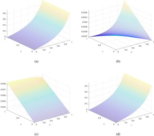
5. Sensitivity analysis

The sensitivity analysis is examined of some of the parameters which are used in the considered system. With the help method we identify the parameters that have a significant effect on the basic reproduction number. The approach of Chintis [48] is utilized to calculate the sensitivity index of ${\mathfrak{R}}_C$. Specifically, the sensitivity index ${\mathrm{\Delta }}_h^{{\mathfrak{R}}_C}$ of a parameter h is presented by the formula ${\mathrm{\Delta }}_h^{{\mathfrak{R}}_C}=\frac{\mathrm{\partial }{\mathfrak{R}}_C}{\mathrm{\partial }k}\frac{h}{{\mathfrak{R}}_C}$. Figure 1(a) represents the sensitivity of the parameter λ with respect to ${\mathfrak{R}}_C$ is depicted. It demonstrates how variations in λ impact the value of ${\mathfrak{R}}_C$. Figure 1(b) shows the sensitivity of the parameter ν with respect to ${\mathfrak{R}}_C$. It indicates the influence of changes in ν on the value of ${\mathfrak{R}}_C$. Similarly, Figure 1(c,d), respectively, shows the sensitivity analysis of the parameters ${\psi }_v$ and ${\psi }_{\gamma }$ in relation to ${\mathfrak{R}}_C$. They provide insights into how modifications in these parameters affect the value of ${\mathfrak{R}}_C$.

6. Qualitative analysis

Now, we seek the existence and uniqueness of solutions for the proposed system, which are essential for the study of dynamical systems. To achieve this, we employ the fixed point approach [49]. Using the differentiability of the integral, the proposed model (3(3) $\begin{array}{rl}{}_0^{FFABC}{D}_t^{\rho ,\kappa }{I}_{\mathcal{S}}\left(t\right)& =\nu \mathrm{\Psi }-{\lambda }_{I_{\mathcal{S}}}\left(t\right)I_{\mathcal{S}}{I}_{\mathcal{C}}\left(t\right)+\theta {\psi }_{I_{\mathcal{T}}}{I}_{\mathcal{T}}\left(t\right)-\gamma I_{\mathcal{S}}\left(t\right),\\ {}_0^{FFABC}{D}_t^{\rho ,\kappa }{I}_{\mathcal{R}}\left(t\right)& ={\lambda }_{I_{\mathcal{S}}}{I}_{\mathcal{S}}\left(t\right)+{\lambda }_{I_{\mathcal{R}}}{I}_{\mathcal{R}}\left(t\right)I_{\mathcal{C}}\left(t\right)-({\psi }_{I_{\mathcal{R}}}+\gamma )I_{\mathcal{R}}\left(t\right),\\ {}_0^{FFABC}{D}_t^{\rho ,\kappa }{I}_{\mathcal{C}}\left(t\right)& =\text{β}{\psi }_{I_{\mathcal{R}}}{I}_{\mathcal{R}}\left(t\right)-{\lambda }_{I_{\mathcal{R}}}{I}_{\mathcal{R}}\left(t\right)I_{\mathcal{C}}\left(t\right)-({\psi }_{I_{\mathcal{C}}}+\gamma )I_{\mathcal{C}}\left(t\right),\\ {}_0^{FFABC}{D}_t^{\rho ,\kappa }{I}_{\mathcal{P}}\left(t\right)& ={\psi }_{I_{\mathcal{C}}}{I}_{\mathcal{C}}\left(t\right)-({\psi }_{I_{\mathcal{P}}}+\gamma )I_{\mathcal{P}}\left(t\right),\\ {}_0^{FFABC}{D}_t^{\rho ,\kappa }{I}_{\mathcal{T}}\left(t\right)& ={\psi }_{I_{\mathcal{P}}}{I}_{\mathcal{P}}\left(t\right)+(1-\lambda ){\psi }_{I_{\mathcal{R}}}{I}_{\mathcal{R}}\left(t\right)-(\gamma +{\psi }_{I_{\mathcal{T}}})I_{\mathcal{T}}\left(t\right),\\ {}_0^{FFABC}{D}_t^{\rho ,\kappa }{I}_{\mathcal{I}}\left(t\right)& =(1-\nu )\mathrm{\Phi }+(1-\theta ){\psi }_{I_{\mathcal{T}}}{I}_{\mathcal{T}}\left(t\right)-\gamma I_{\mathcal{I}}\left(t\right).\end{array}$(3) ) can be expressed as: (6) $\{\begin{array}{rl}{}_0^{FFABC}{D}_t^{\rho }{I}_{\mathcal{S}}\left(t\right)& =\kappa t^{\kappa -1}\left({ϝ}_1\right(t,I_{\mathcal{S}})=\nu \mathrm{\Psi }-{\lambda }_{I_{\mathcal{S}}}(t\left)I_{\mathcal{S}}{I}_{\mathcal{C}}\right(t)+\theta {\psi }_{I_{\mathcal{T}}}{I}_{\mathcal{T}}(t)-\gamma I_{\mathcal{S}}(t),\\ {}_0^{FFABC}{D}_t^{\rho }{I}_{\mathcal{R}}\left(t\right)& =\kappa t^{\kappa -1}\left({ϝ}_2\right(t,I_{\mathcal{R}})={\lambda }_{I_{\mathcal{S}}}{I}_{\mathcal{S}}(t)+{\lambda }_{I_{\mathcal{R}}}{I}_{\mathcal{R}}(t\left)I_{\mathcal{C}}\right(t)-({\psi }_{I_{\mathcal{R}}}+\gamma \left)I_{\mathcal{R}}\right(t),\\ {}_0^{FFABC}{D}_t^{\rho }{I}_{\mathcal{C}}\left(t\right)& =\kappa t^{\kappa -1}\left({ϝ}_2\right(t,I_{\mathcal{C}})=\text{β}{\psi }_{I_{\mathcal{R}}}{I}_{\mathcal{R}}(t)-{\lambda }_{I_{\mathcal{R}}}{I}_{\mathcal{R}}(t\left)I_{\mathcal{C}}\right(t)-({\psi }_{I_{\mathcal{C}}}+\gamma \left)I_{\mathcal{C}}\right(t),\\ {}_0^{FFABC}{D}_t^{\rho }{I}_{\mathcal{P}}\left(t\right)& =\kappa t^{\kappa -1}\left({ϝ}_4\right(t,I_{\mathcal{P}})={\psi }_{I_{\mathcal{C}}}{I}_{\mathcal{C}}(t)-({\psi }_{I_{\mathcal{P}}}+\gamma \left)I_{\mathcal{P}}\right(t),\\ {}_0^{FFABC}{D}_t^{\rho }{I}_{\mathcal{I}}\left(t\right)& =\kappa t^{\kappa -1}\left({ϝ}_5\right(t,I_{\mathcal{I}})={\psi }_{I_{\mathcal{P}}}{I}_{\mathcal{P}}(t)+(1-\lambda \left){\psi }_{I_{\mathcal{R}}}{I}_{\mathcal{R}}\right(t)-(\gamma +{\psi }_{I_{\mathcal{T}}}\left)I_{\mathcal{T}}\right(t),\\ {}_0^{FFABC}{D}_t^{\rho }{I}_{\mathcal{T}}\left(t\right)& =\kappa t^{\kappa -1}\left({ϝ}_6\right(t,I_{\mathcal{T}})=(1-\nu )\mathrm{\Phi }+(1-\theta \left){\psi }_{I_{\mathcal{T}}}{I}_{\mathcal{T}}\right(t)-\gamma I_{\mathcal{I}}(t).\end{array}$(6) Setting (7) ${\mathcal{G}}_k=\underset{C[J,J_k]}{sup}|{ϝ}_k(t,I_{\mathcal{S}},I_{\mathcal{R}},I_{\mathcal{C}},I_{\mathcal{P}},I_{\mathcal{I}},I_{\mathcal{T}})|=||{ϝ}_k(t,I_{\mathcal{S}},I_{\mathcal{R}},I_{\mathcal{C}},I_{\mathcal{P}},I_{\mathcal{I}},I_{\mathcal{T}})||,$(7) where k = 1, 2,.., 6, and (8) $C[J,d_k]=[t-J,t+J]\times [v-J_k,v+J_k]=\mathcal{U}\times {\mathcal{U}}_k,\mathrm{w}\mathrm{h}\mathrm{e}\mathrm{r}\mathrm{e}k=1,\dots ,6.$(8) Here, defining a norm on $C[J,J_k]$, by using Fixed point theorem of Banach for $k=1,\dots ,6.$ As (9) $||\mathsf{Q}\left(t\right)||=su{p}_{t\in X}|{ϝ}_k\left(t\right)|,\mathrm{w}\mathrm{h}\mathrm{e}\mathrm{r}\mathrm{e}X=[t-J,t+J].$(9) For simplicity express Equation (6(6) $\{\begin{array}{rl}{}_0^{FFABC}{D}_t^{\rho }{I}_{\mathcal{S}}\left(t\right)& =\kappa t^{\kappa -1}\left({ϝ}_1\right(t,I_{\mathcal{S}})=\nu \mathrm{\Psi }-{\lambda }_{I_{\mathcal{S}}}(t\left)I_{\mathcal{S}}{I}_{\mathcal{C}}\right(t)+\theta {\psi }_{I_{\mathcal{T}}}{I}_{\mathcal{T}}(t)-\gamma I_{\mathcal{S}}(t),\\ {}_0^{FFABC}{D}_t^{\rho }{I}_{\mathcal{R}}\left(t\right)& =\kappa t^{\kappa -1}\left({ϝ}_2\right(t,I_{\mathcal{R}})={\lambda }_{I_{\mathcal{S}}}{I}_{\mathcal{S}}(t)+{\lambda }_{I_{\mathcal{R}}}{I}_{\mathcal{R}}(t\left)I_{\mathcal{C}}\right(t)-({\psi }_{I_{\mathcal{R}}}+\gamma \left)I_{\mathcal{R}}\right(t),\\ {}_0^{FFABC}{D}_t^{\rho }{I}_{\mathcal{C}}\left(t\right)& =\kappa t^{\kappa -1}\left({ϝ}_2\right(t,I_{\mathcal{C}})=\text{β}{\psi }_{I_{\mathcal{R}}}{I}_{\mathcal{R}}(t)-{\lambda }_{I_{\mathcal{R}}}{I}_{\mathcal{R}}(t\left)I_{\mathcal{C}}\right(t)-({\psi }_{I_{\mathcal{C}}}+\gamma \left)I_{\mathcal{C}}\right(t),\\ {}_0^{FFABC}{D}_t^{\rho }{I}_{\mathcal{P}}\left(t\right)& =\kappa t^{\kappa -1}\left({ϝ}_4\right(t,I_{\mathcal{P}})={\psi }_{I_{\mathcal{C}}}{I}_{\mathcal{C}}(t)-({\psi }_{I_{\mathcal{P}}}+\gamma \left)I_{\mathcal{P}}\right(t),\\ {}_0^{FFABC}{D}_t^{\rho }{I}_{\mathcal{I}}\left(t\right)& =\kappa t^{\kappa -1}\left({ϝ}_5\right(t,I_{\mathcal{I}})={\psi }_{I_{\mathcal{P}}}{I}_{\mathcal{P}}(t)+(1-\lambda \left){\psi }_{I_{\mathcal{R}}}{I}_{\mathcal{R}}\right(t)-(\gamma +{\psi }_{I_{\mathcal{T}}}\left)I_{\mathcal{T}}\right(t),\\ {}_0^{FFABC}{D}_t^{\rho }{I}_{\mathcal{T}}\left(t\right)& =\kappa t^{\kappa -1}\left({ϝ}_6\right(t,I_{\mathcal{T}})=(1-\nu )\mathrm{\Phi }+(1-\theta \left){\psi }_{I_{\mathcal{T}}}{I}_{\mathcal{T}}\right(t)-\gamma I_{\mathcal{I}}(t).\end{array}$(6) ) as (10) $\begin{array}{rl}{}_0^{FFABC}{D}_t^{\rho }\mathsf{Q}\left(t\right)& =\kappa t^{\kappa -1}\mathbb{K}(t,\mathsf{Q}(t\left)\right)\\ \mathsf{Q}\left(0\right)& ={\mathsf{Q}}_0.\end{array}$(10) Where (11) $\mathsf{Q}\left(t\right)=\{\begin{array}{l}{I}_{\mathcal{S}}\left(t\right),\\ I_{\mathcal{R}}\left(t\right),\\ I_{\mathcal{C}}\left(t\right),\\ I_{\mathcal{P}}\left(t\right),\\ I_{\mathcal{T}}\left(t\right),\\ I_{\mathcal{I}}\left(t\right).\end{array}\mathsf{Q}\left(0\right)=\{\begin{array}{l}{I}_{\mathcal{S}}\left(0\right),\\ I_{\mathcal{R}}\left(0\right),\\ I_{\mathcal{C}}\left(0\right),\\ I_{\mathcal{P}}\left(0\right),\\ I_{\mathcal{T}}\left(0\right),\\ I_{\mathcal{I}}\left(0\right).\end{array}\mathbb{K}(t,\mathsf{Q}(t\left)\right)=\{\begin{array}{l}{ϝ}_1(t,I_{\mathcal{S}},I_{\mathcal{R}},I_{\mathcal{C}},I_{\mathcal{P}},I_{\mathcal{I}},I_{\mathcal{T}}),\\ {ϝ}_2(t,I_{\mathcal{S}},I_{\mathcal{R}},I_{\mathcal{C}},I_{\mathcal{P}},I_{\mathcal{I}},I_{\mathcal{T}}),\\ {ϝ}_3(t,I_{\mathcal{S}},I_{\mathcal{R}},I_{\mathcal{C}},I_{\mathcal{P}},I_{\mathcal{I}},I_{\mathcal{T}}),\\ {ϝ}_4(t,I_{\mathcal{S}},I_{\mathcal{R}},I_{\mathcal{C}},I_{\mathcal{P}},I_{\mathcal{I}},I_{\mathcal{T}}),\\ {ϝ}_5(t,I_{\mathcal{S}},I_{\mathcal{R}},I_{\mathcal{C}},I_{\mathcal{P}},I_{\mathcal{I}},I_{\mathcal{T}}),\\ {ϝ}_6(t,I_{\mathcal{S}},I_{\mathcal{R}},I_{\mathcal{C}},I_{\mathcal{P}},I_{\mathcal{I}},I_{\mathcal{T}}).\end{array}$(11) Using fractal-fractional-integration to Equation (10(10) $\begin{array}{rl}{}_0^{FFABC}{D}_t^{\rho }\mathsf{Q}\left(t\right)& =\kappa t^{\kappa -1}\mathbb{K}(t,\mathsf{Q}(t\left)\right)\\ \mathsf{Q}\left(0\right)& ={\mathsf{Q}}_0.\end{array}$(10) ), we get (12) $\mathsf{Q}\left(t\right)=\mathsf{Q}\left(0\right)+\frac{\kappa (1-\rho )t^{\kappa -1}}{M\left(\rho \right)}\mathbb{K}(t,\mathsf{Q}(t\left)\right)+\frac{\kappa \rho }{M\left(\rho \right)}{\int }_0^t{u}^{\rho -1}\mathbb{K}(u,\mathsf{Q}(u\left)\right)\mathrm{d}u.$(12) Now we defining the Picard's operator which as $\mathcal{T}:C(X,X_1,X_2,X_3,X_4,X_5,X_6)\to C(X,X_1,X_2,X_3,X_4,X_5,X_6).$From Equations (10(10) $\begin{array}{rl}{}_0^{FFABC}{D}_t^{\rho }\mathsf{Q}\left(t\right)& =\kappa t^{\kappa -1}\mathbb{K}(t,\mathsf{Q}(t\left)\right)\\ \mathsf{Q}\left(0\right)& ={\mathsf{Q}}_0.\end{array}$(10) ) and (12(12) $\mathsf{Q}\left(t\right)=\mathsf{Q}\left(0\right)+\frac{\kappa (1-\rho )t^{\kappa -1}}{M\left(\rho \right)}\mathbb{K}(t,\mathsf{Q}(t\left)\right)+\frac{\kappa \rho }{M\left(\rho \right)}{\int }_0^t{u}^{\rho -1}\mathbb{K}(u,\mathsf{Q}(u\left)\right)\mathrm{d}u.$(12) ), $\mathcal{T}$ is formulated as (13) $\mathcal{T}\left(\mathsf{Q}\right(t\left)\right)=\mathsf{Q}\left(0\right)+\frac{\kappa (1-\rho )t^{\kappa -1}}{M\left(\rho \right)}\mathbb{K}(t,\mathsf{Q}(t\left)\right)+\frac{\kappa \rho }{M\left(\rho \right)}{\int }_0^t{u}^{\rho -1}\mathbb{K}(u,\mathsf{Q}(u\left)\right)\mathrm{d}u.$(13) Further, we considered $\mathsf{Q}\left(t\right)$ obeys the condition as given $||\mathsf{Q}||\le max(J,J_1,J_2,J_3,J_4,J_5,J_6),$so $\begin{array}{rl}||\mathcal{T}\left(\mathsf{Q}\right(t\left)\right)-\mathsf{Q}\left(0\right)||& =\underset{t\in X}{sup}\left|\frac{\kappa (1-\rho )t^{\kappa -1}}{M\left(\rho \right)}\mathbb{K}\right(t,\mathsf{Q}\left(t\right))+\frac{\kappa \rho }{M\left(\rho \right)}{\int }_0^t{u}^{\rho -1}\mathbb{K}(u,\mathsf{Q}\left(u\right)\left)\mathrm{d}u\right|\\ & \le \frac{\kappa (1-\rho )T^{\kappa -1}}{M\left(\rho \right)}||\mathbb{K}(t,\mathsf{Q}(t\left)\right)||+\frac{\kappa \rho }{M\left(\rho \right)}{\int }_0^t{u}^{\rho -1}||\mathbb{K}(u,\mathsf{Q}(u\left)\right)||\mathrm{d}u\\ & \le (\frac{\kappa (1-\rho )T^{\kappa -1}}{M\left(\rho \right)}+\frac{\kappa T^{\rho }}{M\left(\rho \right)})\mathcal{G},\mathcal{G}=max\left({\mathcal{G}}_k\right)\mathrm{f}\mathrm{o}\mathrm{r}k=1,\dots ,6,\\ & <\mathcal{G}J\le max(J,J_1,J_2,J_3,J_4,J_5,J_6)=\overline{J},T=sup\{|t|:t\in X\}.\end{array}$Where $(\frac{\kappa (1-\rho )T^{\kappa -1}}{M\left(\rho \right)}+\frac{\kappa T^{\rho }}{M\left(\rho \right)})<J$ and $J<\frac{\overline{J}}{\mathcal{G}}$.

Figure 1. The plots show sensitivity analysis of different parameters with the basic reproductive number ${\mathfrak{R}}_C$.

Next, we will assess the following equation to see whether our model is unique. (14) $||\mathcal{T}{\mathsf{Q}}_1-\mathcal{T}{\mathsf{Q}}_2||=\underset{t\in X}{sup}|{\mathsf{Q}}_1-{\mathsf{Q}}_2|,$(14) from Equations (13(13) $\mathcal{T}\left(\mathsf{Q}\right(t\left)\right)=\mathsf{Q}\left(0\right)+\frac{\kappa (1-\rho )t^{\kappa -1}}{M\left(\rho \right)}\mathbb{K}(t,\mathsf{Q}(t\left)\right)+\frac{\kappa \rho }{M\left(\rho \right)}{\int }_0^t{u}^{\rho -1}\mathbb{K}(u,\mathsf{Q}(u\left)\right)\mathrm{d}u.$(13) ) and (14(14) $||\mathcal{T}{\mathsf{Q}}_1-\mathcal{T}{\mathsf{Q}}_2||=\underset{t\in X}{sup}|{\mathsf{Q}}_1-{\mathsf{Q}}_2|,$(14) ), follows $\begin{array}{rl}& ||\mathcal{T}{\mathsf{Q}}_1-\mathcal{T}{\mathsf{Q}}_2||\\ & =\underset{t\in X}{sup}\left|\mathsf{Q}\right(0)+\frac{\kappa (1-\rho )t^{\kappa -1}}{M\left(\rho \right)}({\mathsf{Q}}_1\left(t\right)-{\mathsf{Q}}_2\left(t\right))+\frac{\kappa \rho }{M\left(\rho \right)}{\int }_0^t{u}^{\rho -1}({\mathsf{Q}}_1\left(t\right)-{\mathsf{Q}}_2\left(t\right)\left)\mathrm{d}u\right|\\ & \le \frac{\kappa (1-\rho )T^{\kappa -1}}{M\left(\rho \right)}\varpi \underset{t\in X}{sup}|\left({\mathsf{Q}}_1\right(t)-{\mathsf{Q}}_2(t\left)\right)|\\ & +\frac{\kappa \rho \varpi }{M\left(\rho \right)}\underset{t\in X}{sup}{\int }_0^t{u}^{\rho -1}|\left({\mathsf{Q}}_1\right(u)-{\mathsf{Q}}_2(u\left)\right)|\mathrm{d}u,\varpi <1\\ & \le (\frac{\kappa (1-\rho )T^{\kappa -1}}{M\left(\rho \right)}+\frac{\kappa T^{\rho }}{M\left(\rho \right)})\varpi ||{\mathsf{Q}}_1-{\mathsf{Q}}_2||\\ & \le J\varpi ||{\mathsf{Q}}_1-{\mathsf{Q}}_2||.\end{array}$As $\mathbb{K}$ has a contraction which implies that $J\varpi <1$. This also shows that $\mathcal{T}$ is contraction. So we conclude that the proposed model (3(3) $\begin{array}{rl}{}_0^{FFABC}{D}_t^{\rho ,\kappa }{I}_{\mathcal{S}}\left(t\right)& =\nu \mathrm{\Psi }-{\lambda }_{I_{\mathcal{S}}}\left(t\right)I_{\mathcal{S}}{I}_{\mathcal{C}}\left(t\right)+\theta {\psi }_{I_{\mathcal{T}}}{I}_{\mathcal{T}}\left(t\right)-\gamma I_{\mathcal{S}}\left(t\right),\\ {}_0^{FFABC}{D}_t^{\rho ,\kappa }{I}_{\mathcal{R}}\left(t\right)& ={\lambda }_{I_{\mathcal{S}}}{I}_{\mathcal{S}}\left(t\right)+{\lambda }_{I_{\mathcal{R}}}{I}_{\mathcal{R}}\left(t\right)I_{\mathcal{C}}\left(t\right)-({\psi }_{I_{\mathcal{R}}}+\gamma )I_{\mathcal{R}}\left(t\right),\\ {}_0^{FFABC}{D}_t^{\rho ,\kappa }{I}_{\mathcal{C}}\left(t\right)& =\text{β}{\psi }_{I_{\mathcal{R}}}{I}_{\mathcal{R}}\left(t\right)-{\lambda }_{I_{\mathcal{R}}}{I}_{\mathcal{R}}\left(t\right)I_{\mathcal{C}}\left(t\right)-({\psi }_{I_{\mathcal{C}}}+\gamma )I_{\mathcal{C}}\left(t\right),\\ {}_0^{FFABC}{D}_t^{\rho ,\kappa }{I}_{\mathcal{P}}\left(t\right)& ={\psi }_{I_{\mathcal{C}}}{I}_{\mathcal{C}}\left(t\right)-({\psi }_{I_{\mathcal{P}}}+\gamma )I_{\mathcal{P}}\left(t\right),\\ {}_0^{FFABC}{D}_t^{\rho ,\kappa }{I}_{\mathcal{T}}\left(t\right)& ={\psi }_{I_{\mathcal{P}}}{I}_{\mathcal{P}}\left(t\right)+(1-\lambda ){\psi }_{I_{\mathcal{R}}}{I}_{\mathcal{R}}\left(t\right)-(\gamma +{\psi }_{I_{\mathcal{T}}})I_{\mathcal{T}}\left(t\right),\\ {}_0^{FFABC}{D}_t^{\rho ,\kappa }{I}_{\mathcal{I}}\left(t\right)& =(1-\nu )\mathrm{\Phi }+(1-\theta ){\psi }_{I_{\mathcal{T}}}{I}_{\mathcal{T}}\left(t\right)-\gamma I_{\mathcal{I}}\left(t\right).\end{array}$(3) ) possesses a unique root.

7. Ulam Hyer's stability analysis

Here, we study the stability analysis of the proposed model using the Ulam-Hyers type of stability analysis. Let $\vartheta \left(t\right)$ be a perturbation variable relative to the root with $\vartheta \left(0\right)=0$. Then, we can write the perturbed solution as:

• $|\vartheta \left(t\right)|\le ϵifϵ>0,$

• ${}_0^{FFABC}{D}_t^{\rho ,\kappa }\mathsf{Q}\left(t\right)=\mathsf{A}(t,\mathsf{Q}(t\left)\right)+\vartheta \left(t\right)$.

Lemma 7.1

The root of proposed Equation (3(3) $\begin{array}{rl}{}_0^{FFABC}{D}_t^{\rho ,\kappa }{I}_{\mathcal{S}}\left(t\right)& =\nu \mathrm{\Psi }-{\lambda }_{I_{\mathcal{S}}}\left(t\right)I_{\mathcal{S}}{I}_{\mathcal{C}}\left(t\right)+\theta {\psi }_{I_{\mathcal{T}}}{I}_{\mathcal{T}}\left(t\right)-\gamma I_{\mathcal{S}}\left(t\right),\\ {}_0^{FFABC}{D}_t^{\rho ,\kappa }{I}_{\mathcal{R}}\left(t\right)& ={\lambda }_{I_{\mathcal{S}}}{I}_{\mathcal{S}}\left(t\right)+{\lambda }_{I_{\mathcal{R}}}{I}_{\mathcal{R}}\left(t\right)I_{\mathcal{C}}\left(t\right)-({\psi }_{I_{\mathcal{R}}}+\gamma )I_{\mathcal{R}}\left(t\right),\\ {}_0^{FFABC}{D}_t^{\rho ,\kappa }{I}_{\mathcal{C}}\left(t\right)& =\text{β}{\psi }_{I_{\mathcal{R}}}{I}_{\mathcal{R}}\left(t\right)-{\lambda }_{I_{\mathcal{R}}}{I}_{\mathcal{R}}\left(t\right)I_{\mathcal{C}}\left(t\right)-({\psi }_{I_{\mathcal{C}}}+\gamma )I_{\mathcal{C}}\left(t\right),\\ {}_0^{FFABC}{D}_t^{\rho ,\kappa }{I}_{\mathcal{P}}\left(t\right)& ={\psi }_{I_{\mathcal{C}}}{I}_{\mathcal{C}}\left(t\right)-({\psi }_{I_{\mathcal{P}}}+\gamma )I_{\mathcal{P}}\left(t\right),\\ {}_0^{FFABC}{D}_t^{\rho ,\kappa }{I}_{\mathcal{T}}\left(t\right)& ={\psi }_{I_{\mathcal{P}}}{I}_{\mathcal{P}}\left(t\right)+(1-\lambda ){\psi }_{I_{\mathcal{R}}}{I}_{\mathcal{R}}\left(t\right)-(\gamma +{\psi }_{I_{\mathcal{T}}})I_{\mathcal{T}}\left(t\right),\\ {}_0^{FFABC}{D}_t^{\rho ,\kappa }{I}_{\mathcal{I}}\left(t\right)& =(1-\nu )\mathrm{\Phi }+(1-\theta ){\psi }_{I_{\mathcal{T}}}{I}_{\mathcal{T}}\left(t\right)-\gamma I_{\mathcal{I}}\left(t\right).\end{array}$(3) ) being perturb (15) $\begin{array}{rl}{}_0^{FFABC}{D}_t^{\rho ,\kappa }\mathsf{Q}\left(t\right)& =\mathbb{K}(t,\mathsf{Q}(t\left)\right)+\varpi \left(t\right),\\ \mathsf{Q}\left(0\right)& ={\mathsf{Q}}_0,\end{array}$(15) obeys the equation (16) $\begin{array}{rl}& \left|\mathsf{Q}\right(t)-\left[\phantom{{\int }_0^t}{\mathsf{Q}}_0\right(t)-\left(\mathbb{K}\right(t,\mathsf{Q}\left(t\right))+{\varpi }_0(t\left)\right)\frac{\kappa (1-\rho )}{M\left(\rho \right)}{t}^{\kappa -1}\\ & +\frac{\rho \kappa }{M\left(\rho \right)}{\int }_0^t{u}^{\gamma -1}\mathbb{K}(u,\mathsf{Q}(u\left)\right)\mathrm{d}u]|,\\ & \le (\frac{\kappa T^{\rho }}{M\left(\rho \right)}+\frac{\kappa (1-\rho )T^{\kappa -1}}{M\left(\rho \right)})N_{\mathbb{K}},\end{array}$(16)

Proof.

The derivation of 7.1 is easy, so we omit it.

Theorem 7.1

From Equations (10(10) $\begin{array}{rl}{}_0^{FFABC}{D}_t^{\rho }\mathsf{Q}\left(t\right)& =\kappa t^{\kappa -1}\mathbb{K}(t,\mathsf{Q}(t\left)\right)\\ \mathsf{Q}\left(0\right)& ={\mathsf{Q}}_0.\end{array}$(10) ) and (16(16) $\begin{array}{rl}& \left|\mathsf{Q}\right(t)-\left[\phantom{{\int }_0^t}{\mathsf{Q}}_0\right(t)-\left(\mathbb{K}\right(t,\mathsf{Q}\left(t\right))+{\varpi }_0(t\left)\right)\frac{\kappa (1-\rho )}{M\left(\rho \right)}{t}^{\kappa -1}\\ & +\frac{\rho \kappa }{M\left(\rho \right)}{\int }_0^t{u}^{\gamma -1}\mathbb{K}(u,\mathsf{Q}(u\left)\right)\mathrm{d}u]|,\\ & \le (\frac{\kappa T^{\rho }}{M\left(\rho \right)}+\frac{\kappa (1-\rho )T^{\kappa -1}}{M\left(\rho \right)})N_{\mathbb{K}},\end{array}$(16) ) the root of Equation (7(7) ${\mathcal{G}}_k=\underset{C[J,J_k]}{sup}|{ϝ}_k(t,I_{\mathcal{S}},I_{\mathcal{R}},I_{\mathcal{C}},I_{\mathcal{P}},I_{\mathcal{I}},I_{\mathcal{T}})|=||{ϝ}_k(t,I_{\mathcal{S}},I_{\mathcal{R}},I_{\mathcal{C}},I_{\mathcal{P}},I_{\mathcal{I}},I_{\mathcal{T}})||,$(7) ) is Ulam Hyers stable, therefore the solution of the proposed model is Ulam Hyers stable for $\mathcal{Z}<1$. where $\mathcal{Z}=(\frac{\kappa T^{\rho }}{M\left(\rho \right)}+\frac{\kappa (1-\rho )T^{\kappa -1}}{M\left(\rho \right)})N_{\mathbb{K}}.$

Proof.

Let $\mathsf{Q}\in \mathcal{A}$ is unique, and $\tilde{\mathsf{Q}}$ is another zero of (3(3) $\begin{array}{rl}{}_0^{FFABC}{D}_t^{\rho ,\kappa }{I}_{\mathcal{S}}\left(t\right)& =\nu \mathrm{\Psi }-{\lambda }_{I_{\mathcal{S}}}\left(t\right)I_{\mathcal{S}}{I}_{\mathcal{C}}\left(t\right)+\theta {\psi }_{I_{\mathcal{T}}}{I}_{\mathcal{T}}\left(t\right)-\gamma I_{\mathcal{S}}\left(t\right),\\ {}_0^{FFABC}{D}_t^{\rho ,\kappa }{I}_{\mathcal{R}}\left(t\right)& ={\lambda }_{I_{\mathcal{S}}}{I}_{\mathcal{S}}\left(t\right)+{\lambda }_{I_{\mathcal{R}}}{I}_{\mathcal{R}}\left(t\right)I_{\mathcal{C}}\left(t\right)-({\psi }_{I_{\mathcal{R}}}+\gamma )I_{\mathcal{R}}\left(t\right),\\ {}_0^{FFABC}{D}_t^{\rho ,\kappa }{I}_{\mathcal{C}}\left(t\right)& =\text{β}{\psi }_{I_{\mathcal{R}}}{I}_{\mathcal{R}}\left(t\right)-{\lambda }_{I_{\mathcal{R}}}{I}_{\mathcal{R}}\left(t\right)I_{\mathcal{C}}\left(t\right)-({\psi }_{I_{\mathcal{C}}}+\gamma )I_{\mathcal{C}}\left(t\right),\\ {}_0^{FFABC}{D}_t^{\rho ,\kappa }{I}_{\mathcal{P}}\left(t\right)& ={\psi }_{I_{\mathcal{C}}}{I}_{\mathcal{C}}\left(t\right)-({\psi }_{I_{\mathcal{P}}}+\gamma )I_{\mathcal{P}}\left(t\right),\\ {}_0^{FFABC}{D}_t^{\rho ,\kappa }{I}_{\mathcal{T}}\left(t\right)& ={\psi }_{I_{\mathcal{P}}}{I}_{\mathcal{P}}\left(t\right)+(1-\lambda ){\psi }_{I_{\mathcal{R}}}{I}_{\mathcal{R}}\left(t\right)-(\gamma +{\psi }_{I_{\mathcal{T}}})I_{\mathcal{T}}\left(t\right),\\ {}_0^{FFABC}{D}_t^{\rho ,\kappa }{I}_{\mathcal{I}}\left(t\right)& =(1-\nu )\mathrm{\Phi }+(1-\theta ){\psi }_{I_{\mathcal{T}}}{I}_{\mathcal{T}}\left(t\right)-\gamma I_{\mathcal{I}}\left(t\right).\end{array}$(3) ), then one follows $\begin{array}{rl}|\mathsf{Q}\left(t\right)-\tilde{\mathsf{Q}}\left(t\right)|& =\left|\mathsf{Q}\right(t)-\left({\mathsf{Q}}_0\right(t)+(\mathbb{K}(t,\tilde{\mathsf{Q}}(t\left)\right)-{\mathbb{K}}_0\left(t\right))\frac{\kappa (1-\rho )}{M\left(\rho \right)}{t}^{\kappa -1}\\ & +\frac{\rho \kappa }{M\left(\rho \right)}{\int }_0^t{u}^{\rho -1}\mathbb{K}(u,\tilde{\mathsf{Q}}(u\left)\right)\mathrm{d}u)|\\ & \le \left|\mathsf{Q}\right(t)-\left({\mathsf{Q}}_0\right(t)+(\mathbb{K}(t,\mathsf{Q}(t\left)\right)-{\mathbb{K}}_0\left(t\right))\frac{\kappa (1-\rho )}{M\left(\rho \right)}{t}^{\kappa -1}\\ & +\frac{\rho \kappa }{M\left(\rho \right)}{\int }_0^t{u}^{\rho -1}\mathbb{K}(u,\mathsf{Q}(u\left)\right)\mathrm{d}u)|\\ & +|\left({\mathsf{Q}}_0\right(t)+(\mathbb{K}(t,\mathsf{Q}(t\left)\right)-{\mathbb{K}}_0\left(t\right))\frac{\kappa (1-\rho )}{M\left(\rho \right)}{t}^{\kappa -1}\\ & +\frac{\rho \kappa }{M\left(\rho \right)}{\int }_0^t{u}^{\rho -1}\mathbb{K}(u,\mathsf{Q}(u\left)\right)\mathrm{d}u)\\ & -\left({\mathsf{Q}}_0\right(t)+(\mathbb{K}(t,\tilde{\mathsf{Q}}(t\left)\right)-{\mathbb{K}}_0\left(t\right))\frac{\kappa (1-\rho )}{M\left(\rho \right)}{t}^{\kappa -1}\\ & +\frac{\rho \kappa }{M\left(\rho \right)}{\int }_0^t{u}^{\rho -1}\mathbb{K}(u,\tilde{\mathsf{Q}}(u\left)\right)\mathrm{d}u)|\\ & \le {\mathrm{\wp }}_{\rho ,\kappa }+\frac{\kappa (1-\rho )T^{\kappa -1}{N}_{\mathbb{K}}}{M\left(\rho \right)}||\mathsf{Q}-\tilde{\mathsf{Q}}||+\frac{\kappa T^{\rho }{N}_{\mathbb{K}}}{M\left(\rho \right)}||\mathsf{Q}-\tilde{\mathsf{Q}}||\\ & \le {\mathrm{\wp }}_{\rho ,\kappa }+\mathcal{Z}||\mathsf{Q}-\tilde{\mathsf{Q}}||.\end{array}$Therefore, from the above terms $||\mathsf{Q}-\tilde{\mathsf{Q}}||\le \frac{{\mathrm{\wp }}_{\rho ,\kappa }}{1-\mathcal{Z}}||\mathsf{Q}-\tilde{\mathsf{Q}}||.$Which shows the stability of the zero of the proposed model.

8. Approximate scheme

To establish a numerical approach for the proposed problem with FF operator and Mittag-Leffler law, the Adams-Bashforth FF operator with Lagrange interpolating method is used. A numerical method called the Adams-Bashforth method is used to approximately solve fractional and ordinary differential equations (ODEs). The derivative at the current time step is estimated using a mixture of prior function values and their corresponding derivatives. It then updates the function value for the following time step using this derivative estimate. The method's specific coefficients are based on the scheme's order. To do so, the FF integral of (6(6) $\{\begin{array}{rl}{}_0^{FFABC}{D}_t^{\rho }{I}_{\mathcal{S}}\left(t\right)& =\kappa t^{\kappa -1}\left({ϝ}_1\right(t,I_{\mathcal{S}})=\nu \mathrm{\Psi }-{\lambda }_{I_{\mathcal{S}}}(t\left)I_{\mathcal{S}}{I}_{\mathcal{C}}\right(t)+\theta {\psi }_{I_{\mathcal{T}}}{I}_{\mathcal{T}}(t)-\gamma I_{\mathcal{S}}(t),\\ {}_0^{FFABC}{D}_t^{\rho }{I}_{\mathcal{R}}\left(t\right)& =\kappa t^{\kappa -1}\left({ϝ}_2\right(t,I_{\mathcal{R}})={\lambda }_{I_{\mathcal{S}}}{I}_{\mathcal{S}}(t)+{\lambda }_{I_{\mathcal{R}}}{I}_{\mathcal{R}}(t\left)I_{\mathcal{C}}\right(t)-({\psi }_{I_{\mathcal{R}}}+\gamma \left)I_{\mathcal{R}}\right(t),\\ {}_0^{FFABC}{D}_t^{\rho }{I}_{\mathcal{C}}\left(t\right)& =\kappa t^{\kappa -1}\left({ϝ}_2\right(t,I_{\mathcal{C}})=\text{β}{\psi }_{I_{\mathcal{R}}}{I}_{\mathcal{R}}(t)-{\lambda }_{I_{\mathcal{R}}}{I}_{\mathcal{R}}(t\left)I_{\mathcal{C}}\right(t)-({\psi }_{I_{\mathcal{C}}}+\gamma \left)I_{\mathcal{C}}\right(t),\\ {}_0^{FFABC}{D}_t^{\rho }{I}_{\mathcal{P}}\left(t\right)& =\kappa t^{\kappa -1}\left({ϝ}_4\right(t,I_{\mathcal{P}})={\psi }_{I_{\mathcal{C}}}{I}_{\mathcal{C}}(t)-({\psi }_{I_{\mathcal{P}}}+\gamma \left)I_{\mathcal{P}}\right(t),\\ {}_0^{FFABC}{D}_t^{\rho }{I}_{\mathcal{I}}\left(t\right)& =\kappa t^{\kappa -1}\left({ϝ}_5\right(t,I_{\mathcal{I}})={\psi }_{I_{\mathcal{P}}}{I}_{\mathcal{P}}(t)+(1-\lambda \left){\psi }_{I_{\mathcal{R}}}{I}_{\mathcal{R}}\right(t)-(\gamma +{\psi }_{I_{\mathcal{T}}}\left)I_{\mathcal{T}}\right(t),\\ {}_0^{FFABC}{D}_t^{\rho }{I}_{\mathcal{T}}\left(t\right)& =\kappa t^{\kappa -1}\left({ϝ}_6\right(t,I_{\mathcal{T}})=(1-\nu )\mathrm{\Phi }+(1-\theta \left){\psi }_{I_{\mathcal{T}}}{I}_{\mathcal{T}}\right(t)-\gamma I_{\mathcal{I}}(t).\end{array}$(6) ) is taken, which gives: $\{\begin{array}{rl}{}_0^{FFABC}{D}_t^{\rho }{I}_{\mathcal{S}}\left(t\right)& =\kappa t^{\kappa -1}\left({ϝ}_1\right(t,I_{\mathcal{S}}),\\ {}_0^{FFABC}{D}_t^{\rho }{I}_{\mathcal{R}}\left(t\right)& =\kappa t^{\kappa -1}\left({ϝ}_2\right(t,I_{\mathcal{R}}),\\ {}_0^{FFABC}{D}_t^{\rho }{I}_{\mathcal{C}}\left(t\right)& =\kappa t^{\kappa -1}\left({ϝ}_2\right(t,I_{\mathcal{C}}),\\ {}_0^{FFABC}{D}_t^{\rho }{I}_{\mathcal{P}}\left(t\right)& =\kappa t^{\kappa -1}\left({ϝ}_4\right(t,I_{\mathcal{P}}),\\ {}_0^{FFABC}{D}_t^{\rho }{I}_{\mathcal{I}}\left(t\right)& =\kappa t^{\kappa -1}\left({ϝ}_5\right(t,I_{\mathcal{I}}),\\ {}_0^{FFABC}{D}_t^{\rho }{I}_{\mathcal{T}}\left(t\right)& =\kappa t^{\kappa -1}\left({ϝ}_6\right(t,I_{\mathcal{T}}).\end{array}$here ${ϝ}_1,\dots ,{ϝ}_6$ are presented in (6(6) $\{\begin{array}{rl}{}_0^{FFABC}{D}_t^{\rho }{I}_{\mathcal{S}}\left(t\right)& =\kappa t^{\kappa -1}\left({ϝ}_1\right(t,I_{\mathcal{S}})=\nu \mathrm{\Psi }-{\lambda }_{I_{\mathcal{S}}}(t\left)I_{\mathcal{S}}{I}_{\mathcal{C}}\right(t)+\theta {\psi }_{I_{\mathcal{T}}}{I}_{\mathcal{T}}(t)-\gamma I_{\mathcal{S}}(t),\\ {}_0^{FFABC}{D}_t^{\rho }{I}_{\mathcal{R}}\left(t\right)& =\kappa t^{\kappa -1}\left({ϝ}_2\right(t,I_{\mathcal{R}})={\lambda }_{I_{\mathcal{S}}}{I}_{\mathcal{S}}(t)+{\lambda }_{I_{\mathcal{R}}}{I}_{\mathcal{R}}(t\left)I_{\mathcal{C}}\right(t)-({\psi }_{I_{\mathcal{R}}}+\gamma \left)I_{\mathcal{R}}\right(t),\\ {}_0^{FFABC}{D}_t^{\rho }{I}_{\mathcal{C}}\left(t\right)& =\kappa t^{\kappa -1}\left({ϝ}_2\right(t,I_{\mathcal{C}})=\text{β}{\psi }_{I_{\mathcal{R}}}{I}_{\mathcal{R}}(t)-{\lambda }_{I_{\mathcal{R}}}{I}_{\mathcal{R}}(t\left)I_{\mathcal{C}}\right(t)-({\psi }_{I_{\mathcal{C}}}+\gamma \left)I_{\mathcal{C}}\right(t),\\ {}_0^{FFABC}{D}_t^{\rho }{I}_{\mathcal{P}}\left(t\right)& =\kappa t^{\kappa -1}\left({ϝ}_4\right(t,I_{\mathcal{P}})={\psi }_{I_{\mathcal{C}}}{I}_{\mathcal{C}}(t)-({\psi }_{I_{\mathcal{P}}}+\gamma \left)I_{\mathcal{P}}\right(t),\\ {}_0^{FFABC}{D}_t^{\rho }{I}_{\mathcal{I}}\left(t\right)& =\kappa t^{\kappa -1}\left({ϝ}_5\right(t,I_{\mathcal{I}})={\psi }_{I_{\mathcal{P}}}{I}_{\mathcal{P}}(t)+(1-\lambda \left){\psi }_{I_{\mathcal{R}}}{I}_{\mathcal{R}}\right(t)-(\gamma +{\psi }_{I_{\mathcal{T}}}\left)I_{\mathcal{T}}\right(t),\\ {}_0^{FFABC}{D}_t^{\rho }{I}_{\mathcal{T}}\left(t\right)& =\kappa t^{\kappa -1}\left({ϝ}_6\right(t,I_{\mathcal{T}})=(1-\nu )\mathrm{\Phi }+(1-\theta \left){\psi }_{I_{\mathcal{T}}}{I}_{\mathcal{T}}\right(t)-\gamma I_{\mathcal{I}}(t).\end{array}$(6) ), using the integral to the first equation, we have $I_{\mathcal{S}}\left(t\right)=I_{\mathcal{S}}\left(0\right)+\frac{\kappa (1-\rho )t^{\kappa -1}}{M\left(\rho \right)}{ϝ}_1(t,I_{\mathcal{S}})+\frac{\rho \kappa }{M\left(\rho \right)}{\int }_0^t(t-u{)}^{\rho -1}{u}^{\kappa -1}{ϝ}_1(t,I_{\mathcal{S}})\mathrm{d}u,$and considering $t=t_{J+1}$, for $J=0,1,2,\dots .$ $\begin{array}{rl}& I_{\mathcal{S}}\left(t_{J+1}\right)-I_{\mathcal{S}}\left(0\right)\\ & =\frac{\kappa (1-\rho )t_J^{\kappa -1}}{M\left(\rho \right)}{ϝ}_1(t_J,I_{\mathcal{S}}^J(t\left)\right)+\frac{\rho \kappa }{M\left(\rho \right)}{\int }_0^{t_{J+1}}(t_{J+1}-u{)}^{\rho -1}{u}^{\kappa -1}{ϝ}_1(t,I_{\mathcal{S}})\mathrm{d}u,\\ & =\frac{\kappa (1-\rho )t_J^{\kappa -1}}{M\left(\rho \right)}{ϝ}_1(t_J,I_{\mathcal{S}}^J(t\left)\right)+\frac{\rho \kappa }{M\left(\rho \right)}\sum _{i=1}^J{\int }_0^{t_{J+1}}(t_{J+1}-u{)}^{\rho -1}{u}^{\kappa -1}{ϝ}_1(t,I_{\mathcal{S}})\mathrm{d}u,\end{array}$The interpolation polynomial through the approximate function ${ϝ}_1$ on interval $[t_j,t_{J+1}]$, will be ${ϝ}_1\cong \frac{{ϝ}_1}{\mathrm{\Delta }}(t-t_{i-1})-\frac{{\mathbf{\text{R}}}_1}{\mathrm{\Delta }}(t-t_r)$gives (17) $\begin{array}{rl}{I}_{\mathcal{S}}\left(t_{J+1}\right)& =I_{\mathcal{S}}\left(0\right)+\frac{(1-\rho )}{M\left(\rho \right)}\left(t_{J+1}^{\kappa -1}\right)[{ϝ}_1(I_{\mathcal{S}}\left(t_c\right),t_c)]+\frac{\kappa \rho }{M\left(\rho \right)\mathrm{\Gamma }\left(\rho \right)}\sum _{i=0}^J(\frac{{ϝ}_1(I_{\mathcal{S}}\left(t_c\right),t_c)}{\mathrm{\Delta }}\\ & \times {\int }_J^{t_{i+1}}(t-t_{i-1})(t_{i+1}-t{)}^{\rho -1}{t}_J^{\kappa -1}dt\\ & -\frac{{ϝ}_1(I_{\mathcal{S}}\left(t_c\right),t_c)}{\mathrm{\Delta }}{\int }_J^{t_{i+1}}(t-t_i)(t_{J+1}-t{)}^{\rho -1}{t}_J^{\kappa -1}dt),\\ I_{\mathcal{S}}\left(t_{J+1}\right)& =I_{\mathcal{S}}\left(0\right)+\frac{(1-\rho )}{M\left(\rho \right)}\left(t_{J+1}^{\kappa -1}\right)[{ϝ}_1(I_{\mathcal{S}}\left(t_c\right),t_c)]+\frac{\kappa \rho }{M\left(\rho \right)\mathrm{\Gamma }\left(\rho \right)}\\ & \times \sum _{i=0}^J(\frac{{ϝ}_1(I_{\mathcal{S}}\left(t_i\right),t_i)}{\mathrm{\Delta }}{\mathbf{\text{I}}}_{i-1,\rho }-\frac{t_{i-1}^{\kappa -1}{ϝ}_1(I_{\mathcal{S}}\left(t_{i-1}\right),t_{i-1})}{\mathrm{\Delta }}{\mathbf{\text{I}}}_{i,\rho }),\end{array}$(17) simplifying ${\mathbf{\text{I}}}_{i-1,\rho }$ and ${\mathbf{\text{I}}}_{i,\rho }$, we obtain $\begin{array}{rl}{\mathbf{\text{I}}}_{i-1,\rho }& ={\int }_i^{t_{i+1}}(t-t_{i-1})(t_{J+1}-t{)}^{\rho -1}dt,\\ & =-\frac{1}{\rho }[(t_{i+1}-t_{i-1})(t_{J+1}-t_{i+1}{)}^{\sigma }-(t_i-t_{i-1}\left)\right(t_{J+1}-t_i{)}^{\kappa }]\\ & -\frac{1}{\rho (\rho -1)}[(t_{J+1}-t_{i+1}{)}^{\rho +1}-(t_{J+1}-t_i{)}^{\rho +1}],\end{array}$and $\begin{array}{rl}{\mathbf{\text{I}}}_{i,\rho }& ={\int }_i^{t_{i+1}}(t-t_i)(t_{J+1}-t{)}^{\rho -1}dt,\\ & =-\frac{1}{\rho }[(t_{i+1}-t_i)(t_{J+1}-t_{i+1}{)}^{\rho }]\\ & -\frac{1}{\rho (\rho -1)}[(t_{J+1}-t_{i+1}{)}^{\rho +1}-(t_{J+1}-t_i{)}^{\kappa +1}],\end{array}$letting $t_i=i\mathrm{\Delta },$ we have (18) $\begin{array}{rl}{\mathbf{\text{I}}}_{i-1,\rho }& =-\frac{{\mathrm{\Delta }}^{\rho +1}}{\rho }[(i+1-(i-1\left)\right)(c+1-(i+1){)}^{\rho }-(i-(i-1)\left)\right(J+1-i^{\rho })]\\ & -\frac{{\mathrm{\Delta }}^{\rho +1}}{\rho (\rho -1)}[(c+1-(i+1){)}^{\rho +1}-(J+1-i{)}^{\rho +1}],\\ & =\frac{{\mathrm{\Delta }}^{\rho +1}}{\rho (\rho -1)}[-2(\rho +1)(J-i{)}^{\rho }\\ & +(\rho +1)(J+1-i{)}^{\rho }-(J-i{)}^{\rho +1}+(J+1-i{)}^{\rho +1}],\\ & =\frac{{\mathrm{\Delta }}^{\rho +1}}{\rho (\rho -1)}[(J-i{)}^{\rho }(-2(\rho +1)-(J-i))+(J+1-i{)}^{\rho }(\rho +1+J+1-i)],\\ & =\frac{{\mathrm{\Delta }}^{\rho +1}}{\rho (\rho -1)}[(J+1-i{)}^{\rho }(J-i+2+\rho )-(J-i{)}^{\rho }(J-i+2+2\rho )],\end{array}$(18) and (19) $\begin{array}{rl}{\mathbf{\text{I}}}_{i,\rho }& =-\frac{{\mathrm{\Delta }}^{\rho +1}}{\rho }[(J+1-i)(J+1-(i+1){)}^{\rho }]\\ & -\frac{{\mathrm{\Delta }}^{\rho +1}}{\rho (\rho -1)}[(J+1-(i+1){)}^{\rho +1}-(J+1-i{)}^{\rho +1}],\\ & =\frac{{\mathrm{\Delta }}^{\rho +1}}{\rho (\rho -1)}[-(\rho +1)(J-i{)}^{\rho }-(J-i{)}^{\rho +1}+(J+1-i{)}^{\rho +1}],\\ & =\frac{{\mathrm{\Delta }}^{\rho +1}}{\rho (\rho -1)}[(J-i{)}^{\rho }(-(i+1)-(J-i))+(J+1-i{)}^{\rho +1}],\\ & =\frac{{\mathrm{\Delta }}^{\rho +1}}{\rho (\rho -1)}[(J+1-i{)}^{\rho +1}-(J-i{)}^{\rho }(J-i+1+\rho )],\end{array}$(19) On substituting Equations (18(18) $\begin{array}{rl}{\mathbf{\text{I}}}_{i-1,\rho }& =-\frac{{\mathrm{\Delta }}^{\rho +1}}{\rho }[(i+1-(i-1\left)\right)(c+1-(i+1){)}^{\rho }-(i-(i-1)\left)\right(J+1-i^{\rho })]\\ & -\frac{{\mathrm{\Delta }}^{\rho +1}}{\rho (\rho -1)}[(c+1-(i+1){)}^{\rho +1}-(J+1-i{)}^{\rho +1}],\\ & =\frac{{\mathrm{\Delta }}^{\rho +1}}{\rho (\rho -1)}[-2(\rho +1)(J-i{)}^{\rho }\\ & +(\rho +1)(J+1-i{)}^{\rho }-(J-i{)}^{\rho +1}+(J+1-i{)}^{\rho +1}],\\ & =\frac{{\mathrm{\Delta }}^{\rho +1}}{\rho (\rho -1)}[(J-i{)}^{\rho }(-2(\rho +1)-(J-i))+(J+1-i{)}^{\rho }(\rho +1+J+1-i)],\\ & =\frac{{\mathrm{\Delta }}^{\rho +1}}{\rho (\rho -1)}[(J+1-i{)}^{\rho }(J-i+2+\rho )-(J-i{)}^{\rho }(J-i+2+2\rho )],\end{array}$(18) ) and (19(19) $\begin{array}{rl}{\mathbf{\text{I}}}_{i,\rho }& =-\frac{{\mathrm{\Delta }}^{\rho +1}}{\rho }[(J+1-i)(J+1-(i+1){)}^{\rho }]\\ & -\frac{{\mathrm{\Delta }}^{\rho +1}}{\rho (\rho -1)}[(J+1-(i+1){)}^{\rho +1}-(J+1-i{)}^{\rho +1}],\\ & =\frac{{\mathrm{\Delta }}^{\rho +1}}{\rho (\rho -1)}[-(\rho +1)(J-i{)}^{\rho }-(J-i{)}^{\rho +1}+(J+1-i{)}^{\rho +1}],\\ & =\frac{{\mathrm{\Delta }}^{\rho +1}}{\rho (\rho -1)}[(J-i{)}^{\rho }(-(i+1)-(J-i))+(J+1-i{)}^{\rho +1}],\\ & =\frac{{\mathrm{\Delta }}^{\rho +1}}{\rho (\rho -1)}[(J+1-i{)}^{\rho +1}-(J-i{)}^{\rho }(J-i+1+\rho )],\end{array}$(19) ) into Equation (17(17) $\begin{array}{rl}{I}_{\mathcal{S}}\left(t_{J+1}\right)& =I_{\mathcal{S}}\left(0\right)+\frac{(1-\rho )}{M\left(\rho \right)}\left(t_{J+1}^{\kappa -1}\right)[{ϝ}_1(I_{\mathcal{S}}\left(t_c\right),t_c)]+\frac{\kappa \rho }{M\left(\rho \right)\mathrm{\Gamma }\left(\rho \right)}\sum _{i=0}^J(\frac{{ϝ}_1(I_{\mathcal{S}}\left(t_c\right),t_c)}{\mathrm{\Delta }}\\ & \times {\int }_J^{t_{i+1}}(t-t_{i-1})(t_{i+1}-t{)}^{\rho -1}{t}_J^{\kappa -1}dt\\ & -\frac{{ϝ}_1(I_{\mathcal{S}}\left(t_c\right),t_c)}{\mathrm{\Delta }}{\int }_J^{t_{i+1}}(t-t_i)(t_{J+1}-t{)}^{\rho -1}{t}_J^{\kappa -1}dt),\\ I_{\mathcal{S}}\left(t_{J+1}\right)& =I_{\mathcal{S}}\left(0\right)+\frac{(1-\rho )}{M\left(\rho \right)}\left(t_{J+1}^{\kappa -1}\right)[{ϝ}_1(I_{\mathcal{S}}\left(t_c\right),t_c)]+\frac{\kappa \rho }{M\left(\rho \right)\mathrm{\Gamma }\left(\rho \right)}\\ & \times \sum _{i=0}^J(\frac{{ϝ}_1(I_{\mathcal{S}}\left(t_i\right),t_i)}{\mathrm{\Delta }}{\mathbf{\text{I}}}_{i-1,\rho }-\frac{t_{i-1}^{\kappa -1}{ϝ}_1(I_{\mathcal{S}}\left(t_{i-1}\right),t_{i-1})}{\mathrm{\Delta }}{\mathbf{\text{I}}}_{i,\rho }),\end{array}$(17) ), we obtain (20) $\begin{array}{rl}& I_{\mathcal{S}}\left(t_{c+1}\right)\\ & =\{\begin{array}{rl}& I_{\mathcal{S}}\left(0\right)+\frac{(1-\rho )}{M\left(\rho \right)}\left(t_{c+1}^{\kappa -1}\right)[{ϝ}_1(I_{\mathcal{S}}\left(t_J\right),t_J)]\\ & +\frac{\kappa \rho }{M\left(\rho \right)\mathrm{\Gamma }\left(\rho \right)}{\sum }_{i=0}^J(\frac{t_r^{\kappa -1}{ϝ}_1(I_{\mathcal{S}}\left(t_i\right),t_i)}{\mathrm{\Delta }}\\ & \times [\frac{{\mathrm{\Delta }}^{\rho +1}}{\rho (\rho -1)}[(J+1-i{)}^{\rho }(J-i+2+\rho )-(J-i{)}^{\rho }(J-i+2+2\rho )]]\\ & -\frac{t_{i-1}^{\kappa -1}{ϝ}_1(I_{\mathcal{S}}\left(t_{i-1}\right),t_{i-1})}{\mathrm{\Delta }}\\ & [\frac{{\mathrm{\Delta }}^{\rho +1}}{\rho (\rho -1)}[(J+1-i{)}^{\rho +1}-(J-i{)}^{\rho }(J-i+1+\rho )]]).\end{array}\end{array}$(20) Considering the remaining terms of the system as follows: (21) $\begin{array}{rl}& I_{\mathcal{R}}\left(t_{c+1}\right)\\ & =\{\begin{array}{rl}& I_{\mathcal{R}}\left(0\right)+\frac{(1-\rho )}{M\left(\rho \right)}\left(t_{c+1}^{\kappa -1}\right)[{ϝ}_1(I_{\mathcal{R}}\left(t_J\right),t_J)]+\frac{\kappa \rho }{M\left(\rho \right)\mathrm{\Gamma }\left(\rho \right)}\\ & {\sum }_{i=0}^J(\frac{t_r^{\kappa -1}{ϝ}_2(I_{\mathcal{R}}\left(t_i\right),t_i)}{\mathrm{\Delta }}[\frac{{\mathrm{\Delta }}^{\rho +1}}{\rho (\rho -1)}\\ & \times [(J+1-i{)}^{\rho }(J-i+2+\rho )-(J-i{)}^{\rho }(J-i+2+2\rho )]]\\ & -\frac{t_{i-1}^{\kappa -1}{ϝ}_2(I_{\mathcal{R}}\left(t_{i-1}\right),t_{i-1})}{\mathrm{\Delta }}\\ & [\frac{{\mathrm{\Delta }}^{\rho +1}}{\rho (\rho -1)}[(J+1-i{)}^{\rho +1}-(J-i{)}^{\rho }(J-i+1+\rho )]]),\end{array}\end{array}$(21) (22) $\begin{array}{rl}& I_{\mathcal{C}}\left(t_{c+1}\right)\\ & =\{\begin{array}{rl}& I_{\mathcal{C}}\left(0\right)+\frac{(1-\rho )}{M\left(\rho \right)}\left(t_{c+1}^{\kappa -1}\right)[{ϝ}_3(I_{\mathcal{C}}\left(t_J\right),t_J)]+\frac{\kappa \rho }{M\left(\rho \right)\mathrm{\Gamma }\left(\rho \right)}\\ & {\sum }_{i=0}^J(\frac{t_r^{\kappa -1}{ϝ}_3(I_{\mathcal{C}}\left(t_i\right),t_i)}{\mathrm{\Delta }}[\frac{{\mathrm{\Delta }}^{\rho +1}}{\rho (\rho -1)}\\ & \times [(J+1-i{)}^{\rho }(J-i+2+\rho )-(J-i{)}^{\rho }(J-i+2+2\rho )]]\\ & -\frac{t_{i-1}^{\kappa -1}{ϝ}_3(I_{\mathcal{C}}\left(t_{i-1}\right),t_{i-1})}{\mathrm{\Delta }}\\ & [\frac{{\mathrm{\Delta }}^{\rho +1}}{\rho (\rho -1)}[(J+1-i{)}^{\rho +1}-(J-i{)}^{\rho }(J-i+1+\rho )]]),\end{array}\end{array}$(22) (23) $\begin{array}{rl}& I_{\mathcal{P}}\left(t_{c+1}\right)\\ & =\{\begin{array}{rl}& I_{\mathcal{P}}\left(0\right)+\frac{(1-\rho )}{M\left(\rho \right)}\left(t_{c+1}^{\kappa -1}\right)[{ϝ}_4(I_{\mathcal{P}}\left(t_J\right),t_J)]+\frac{\kappa \rho }{M\left(\rho \right)\mathrm{\Gamma }\left(\rho \right)}\\ & \times \sum _{i=0}^J(\frac{t_r^{\kappa -1}{ϝ}_4(I_{\mathcal{P}}\left(t_i\right),t_i)}{\mathrm{\Delta }}[\frac{{\mathrm{\Delta }}^{\rho +1}}{\rho (\rho -1)}\\ & \times [(J+1-i{)}^{\rho }(J-i+2+\rho )-(J-i{)}^{\rho }(J-i+2+2\rho )]]\\ & -\frac{t_{i-1}^{\kappa -1}{ϝ}_4(I_{\mathcal{P}}\left(t_{i-1}\right),t_{i-1})}{\mathrm{\Delta }}\\ & [\frac{{\mathrm{\Delta }}^{\rho +1}}{\rho (\rho -1)}[(J+1-i{)}^{\rho +1}-(J-i{)}^{\rho }(J-i+1+\rho )]]),\end{array}\end{array}$(23) (24) $\begin{array}{rl}& I_{\mathcal{I}}\left(t_{c+1}\right)\\ & =\{\begin{array}{rl}& I_{\mathcal{I}}\left(0\right)+\frac{(1-\rho )}{M\left(\rho \right)}\left(t_{c+1}^{\kappa -1}\right)[{ϝ}_5(I_{\mathcal{I}}\left(t_J\right),t_J)]+\frac{\kappa \rho }{M\left(\rho \right)\mathrm{\Gamma }\left(\rho \right)}\sum _{i=0}^J(\frac{t_r^{\kappa -1}{ϝ}_5(I_{\mathcal{I}}\left(t_i\right),t_i)}{\mathrm{\Delta }}\\ & \times [\frac{{\mathrm{\Delta }}^{\rho +1}}{\rho (\rho -1)}[(J+1-i{)}^{\rho }(J-i+2+\rho )-(J-i{)}^{\rho }(J-i+2+2\rho )]]\\ & -\frac{t_{i-1}^{\kappa -1}{ϝ}_5(I_{\mathcal{I}}\left(t_{i-1}\right),t_{i-1})}{\mathrm{\Delta }}\\ & [\frac{{\mathrm{\Delta }}^{\rho +1}}{\rho (\rho -1)}[(J+1-i{)}^{\rho +1}-(J-i{)}^{\rho }(J-i+1+\rho )]]),\end{array}\end{array}$(24) (25) $\begin{array}{rl}& I_{\mathcal{T}}\left(t_{c+1}\right)\\ & =\{\begin{array}{rl}& I_{\mathcal{T}}\left(0\right)+\frac{(1-\rho )}{M\left(\rho \right)}\left(t_{c+1}^{\kappa -1}\right)[{ϝ}_6(I_{\mathcal{T}}\left(t_J\right),t_J)]+\frac{\kappa \rho }{M\left(\rho \right)\mathrm{\Gamma }\left(\rho \right)}\sum _{i=0}^J(\frac{t_r^{\kappa -1}{ϝ}_6(I_{\mathcal{T}}\left(t_i\right),t_i)}{\mathrm{\Delta }}\\ & \times [\frac{{\mathrm{\Delta }}^{\rho +1}}{\rho (\rho -1)}[(J+1-i{)}^{\rho }(J-i+2+\rho )-(J-i{)}^{\rho }(J-i+2+2\rho )]]\\ & -\frac{t_{i-1}^{\kappa -1}{ϝ}_6(I_{\mathcal{T}}\left(t_{i-1}\right),t_{i-1})}{\mathrm{\Delta }}\\ & [\frac{{\mathrm{\Delta }}^{\rho +1}}{\rho (\rho -1)}[(J+1-i{)}^{\rho +1}-(J-i{)}^{\rho }(J-i+1+\rho )]]),\end{array}\end{array}$(25) are the approximate solution for the considered model (3(3) $\begin{array}{rl}{}_0^{FFABC}{D}_t^{\rho ,\kappa }{I}_{\mathcal{S}}\left(t\right)& =\nu \mathrm{\Psi }-{\lambda }_{I_{\mathcal{S}}}\left(t\right)I_{\mathcal{S}}{I}_{\mathcal{C}}\left(t\right)+\theta {\psi }_{I_{\mathcal{T}}}{I}_{\mathcal{T}}\left(t\right)-\gamma I_{\mathcal{S}}\left(t\right),\\ {}_0^{FFABC}{D}_t^{\rho ,\kappa }{I}_{\mathcal{R}}\left(t\right)& ={\lambda }_{I_{\mathcal{S}}}{I}_{\mathcal{S}}\left(t\right)+{\lambda }_{I_{\mathcal{R}}}{I}_{\mathcal{R}}\left(t\right)I_{\mathcal{C}}\left(t\right)-({\psi }_{I_{\mathcal{R}}}+\gamma )I_{\mathcal{R}}\left(t\right),\\ {}_0^{FFABC}{D}_t^{\rho ,\kappa }{I}_{\mathcal{C}}\left(t\right)& =\text{β}{\psi }_{I_{\mathcal{R}}}{I}_{\mathcal{R}}\left(t\right)-{\lambda }_{I_{\mathcal{R}}}{I}_{\mathcal{R}}\left(t\right)I_{\mathcal{C}}\left(t\right)-({\psi }_{I_{\mathcal{C}}}+\gamma )I_{\mathcal{C}}\left(t\right),\\ {}_0^{FFABC}{D}_t^{\rho ,\kappa }{I}_{\mathcal{P}}\left(t\right)& ={\psi }_{I_{\mathcal{C}}}{I}_{\mathcal{C}}\left(t\right)-({\psi }_{I_{\mathcal{P}}}+\gamma )I_{\mathcal{P}}\left(t\right),\\ {}_0^{FFABC}{D}_t^{\rho ,\kappa }{I}_{\mathcal{T}}\left(t\right)& ={\psi }_{I_{\mathcal{P}}}{I}_{\mathcal{P}}\left(t\right)+(1-\lambda ){\psi }_{I_{\mathcal{R}}}{I}_{\mathcal{R}}\left(t\right)-(\gamma +{\psi }_{I_{\mathcal{T}}})I_{\mathcal{T}}\left(t\right),\\ {}_0^{FFABC}{D}_t^{\rho ,\kappa }{I}_{\mathcal{I}}\left(t\right)& =(1-\nu )\mathrm{\Phi }+(1-\theta ){\psi }_{I_{\mathcal{T}}}{I}_{\mathcal{T}}\left(t\right)-\gamma I_{\mathcal{I}}\left(t\right).\end{array}$(3) ).

9. Numerical simulation

We now present the simulation results for all six agents using available data on arbitrary orders of derivatives and fractal dimension, along with a time duration in days. 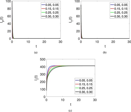The initial values are set as $I_{\mathcal{S}}\left(0\right)=100$, $I_{\mathcal{R}}\left(0\right)=300$, $I_{\mathcal{C}}\left(0\right)=200$, $I_{\mathcal{P}}\left(0\right)=100$, $I_{\mathcal{T}}\left(0\right)=90$, and $I_{\mathcal{I}}\left(0\right)=100$, and the parameters used are listed in Table 1. The graphical representation is done in the sense of the fractal-fractional Atangana–Baleanu derivative. Figure 2(a–f) shows the graphical view of the six compartments of the proposed model for corruption model of the human society. The dynamics is provided under the fractional operator of Caputo along with fractal dimension showing the effects of both parameters. At the beginning, the susceptible population quite decreases but after some it increases and become stable on different fractional orders. The class of risk population slightly increases but after some time it decreases and then become stable. The classes of corrupted population decline for all fractional orders and like this the the punished and transferred population declines. By this result the last class of immune individuals which are free of corruption increases and then become stable. Figures 3(a)–4(c) also show the graphical view of the six compartments of the proposed model for corruption model of the human society. The dynamics is provided under the fractional operator of Atangana–Baleanu along with fractal dimension showing the effects of both parameters. Here only the time duration is increased.

Table 1. Parameters along with numerical values of model (3(3) $\begin{array}{rl}{}_0^{FFABC}{D}_t^{\rho ,\kappa }{I}_{\mathcal{S}}\left(t\right)& =\nu \mathrm{\Psi }-{\lambda }_{I_{\mathcal{S}}}\left(t\right)I_{\mathcal{S}}{I}_{\mathcal{C}}\left(t\right)+\theta {\psi }_{I_{\mathcal{T}}}{I}_{\mathcal{T}}\left(t\right)-\gamma I_{\mathcal{S}}\left(t\right),\\ {}_0^{FFABC}{D}_t^{\rho ,\kappa }{I}_{\mathcal{R}}\left(t\right)& ={\lambda }_{I_{\mathcal{S}}}{I}_{\mathcal{S}}\left(t\right)+{\lambda }_{I_{\mathcal{R}}}{I}_{\mathcal{R}}\left(t\right)I_{\mathcal{C}}\left(t\right)-({\psi }_{I_{\mathcal{R}}}+\gamma )I_{\mathcal{R}}\left(t\right),\\ {}_0^{FFABC}{D}_t^{\rho ,\kappa }{I}_{\mathcal{C}}\left(t\right)& =\text{β}{\psi }_{I_{\mathcal{R}}}{I}_{\mathcal{R}}\left(t\right)-{\lambda }_{I_{\mathcal{R}}}{I}_{\mathcal{R}}\left(t\right)I_{\mathcal{C}}\left(t\right)-({\psi }_{I_{\mathcal{C}}}+\gamma )I_{\mathcal{C}}\left(t\right),\\ {}_0^{FFABC}{D}_t^{\rho ,\kappa }{I}_{\mathcal{P}}\left(t\right)& ={\psi }_{I_{\mathcal{C}}}{I}_{\mathcal{C}}\left(t\right)-({\psi }_{I_{\mathcal{P}}}+\gamma )I_{\mathcal{P}}\left(t\right),\\ {}_0^{FFABC}{D}_t^{\rho ,\kappa }{I}_{\mathcal{T}}\left(t\right)& ={\psi }_{I_{\mathcal{P}}}{I}_{\mathcal{P}}\left(t\right)+(1-\lambda ){\psi }_{I_{\mathcal{R}}}{I}_{\mathcal{R}}\left(t\right)-(\gamma +{\psi }_{I_{\mathcal{T}}})I_{\mathcal{T}}\left(t\right),\\ {}_0^{FFABC}{D}_t^{\rho ,\kappa }{I}_{\mathcal{I}}\left(t\right)& =(1-\nu )\mathrm{\Phi }+(1-\theta ){\psi }_{I_{\mathcal{T}}}{I}_{\mathcal{T}}\left(t\right)-\gamma I_{\mathcal{I}}\left(t\right).\end{array}$(3) ).

Parameter	Value	Parameter	Value
ν	0.0431	Ψ	70
${\lambda }_{I_{\mathcal{S}}}$	0.01025	θ	0.043
γ	0.0163	${\xi }_{I_{\mathcal{T}}}$	0.45
${\lambda }_{I_{\mathcal{R}}}$	0.003	${\psi }_{I_{\mathcal{R}}}$	0.0023
β	0.51	${\psi }_{I_{\mathcal{C}}}$	0.082
${\xi }_{I_{\mathcal{P}}}$	0.21

Figure 2. Graphical view of all agent of the human society on different arbitrary orders $\rho =\kappa =0.75,0.85,0.95,1$ and time duration.

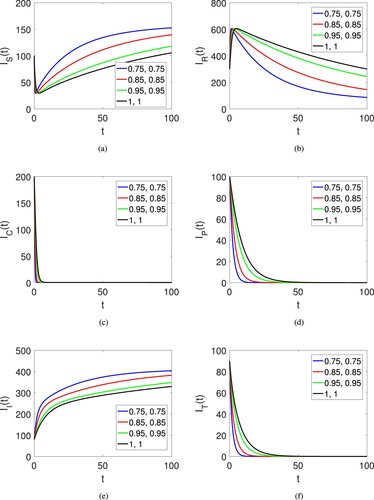
Figure 3. Graphical view of the three agent for the corruption model of the human society on different arbitrary orders $\rho =\kappa =0.75,0.85,0.95,1$ and time duration.

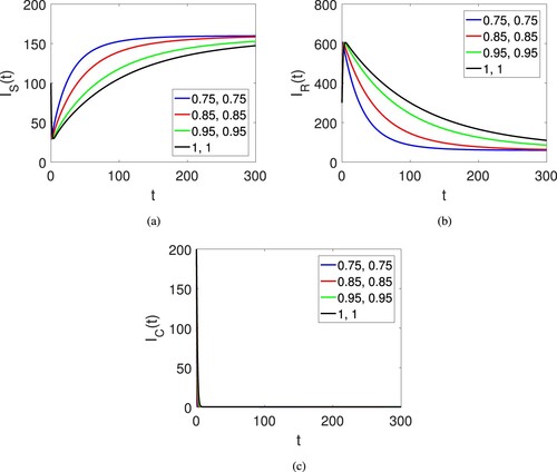
Figure 4. Graphical view of the three agent for the corruption model of the human society on different arbitrary orders $\rho =\kappa =0.75,0.85,0.95,1$ and time duration.

Next, Figure 5(a–f) also shows the graphical view of the six compartments of the proposed model for corruption model of the human society on small fractional orders and fractal dimensions with initial data $I_{\mathcal{S}}\left(0\right)=100,I_{\mathcal{R}}\left(0\right)=300,I_{\mathcal{C}}\left(0\right)=200,I_{\mathcal{P}}\left(0\right)=100,I_{\mathcal{T}}\left(0\right)=90,I_{\mathcal{T}}\left(0\right)=80$. The dynamics is provided under the fractional operator of Atangana Baleanu along with fractal dimension showing the effects of both parameters. Here only the time duration is increased. Next, Figures 6(a)–7(c) also show the graphical representation of the six compartments of the proposed model for corruption model of the human society on very small fractional orders and fractal dimensions. The dynamics is provided under the fractional operator of Atangana Baleanu along with fractal dimension showing the effects of both parameters. Here only impact of order of derivative is tested.

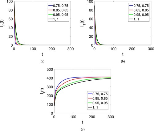
Figure 5. Graphical view of all agent of the human society on different arbitrary orders $\rho =\kappa =0.35,0.45,0.55,0.65$ and time duration.

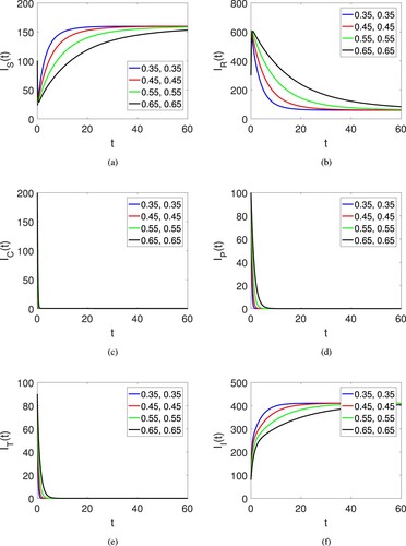
Figure 6. Graphical view of the three agent of the human society on different arbitrary orders $\rho =\kappa =0.05,0.15,0.25,0.30$ and time duration.

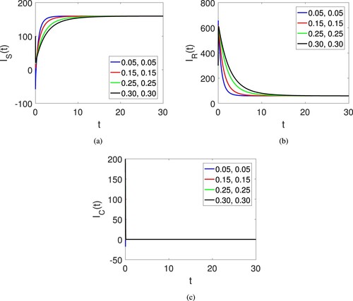
Figure 7. Graphical view of the three agent of the human society on different arbitrary orders $\rho =\kappa =0.05,0.15,0.25,0.30$ and time duration.

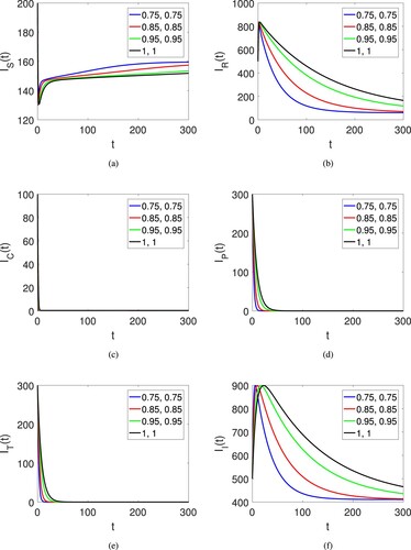
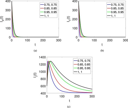
Next, Figure 8(a–f) also shows the graphical view of the six compartments of the proposed model for corruption model of the human society on large fractional orders and fractal dimensions along with another set of initial data $I_{\mathcal{S}}\left(0\right)=200,I_{\mathcal{R}}\left(0\right)=500,I_{\mathcal{C}}\left(0\right)=100,I_{\mathcal{P}}\left(0\right)=300,I_{\mathcal{T}}\left(0\right)=300,I_{\mathcal{T}}\left(0\right)=500$. The dynamics is provided under the fractional operator of Atangana Baleanu along with fractal dimension showing the effects of both parameters. Here only the quantities are converging to the equilibrium points.

Figure 8. Graphical view of the all agent of the human society on different arbitrary orders $\rho =\kappa =0.75,0.85,0.95,1$ on another set of initial data and time duration.

Next, Figures 9(a)–10(c) also show the graphical view of the six compartments of the proposed model for corruption model of the human society on fractional orders and fractal dimensions along with variation in the initial data $I_{\mathcal{S}}\left(0\right)=180,I_{\mathcal{R}}\left(0\right)=500,I_{\mathcal{C}}\left(0\right)=300,I_{\mathcal{P}}\left(0\right)=400,I_{\mathcal{T}}\left(0\right)=400,I_{\mathcal{T}}\left(0\right)=600$. The dynamics is provided under the fractional operator of Atangana Baleanu along with fractal dimension showing the effects of both parameters. Here only the time duration is increased.

Figure 9. Graphical view of the three agent of the human society on different arbitrary orders $\rho =\kappa =0.75,0.85,0.95,1$ on another set of initial data and time duration.

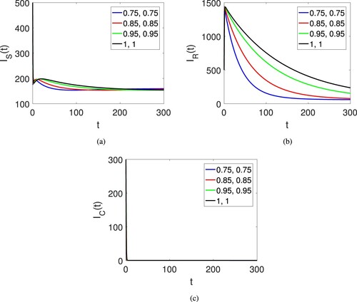
Figure 10. Graphical view of the three agent of the human society on different arbitrary orders $\rho =\kappa =0.75,0.85,0.95,1$ on another set of initial data and time duration.

10. Conclusion

In this research article, we have obtained comparable results for controlling corruption in human society by utilizing a more informative derivative of fractal dimensions and fractional order to describe the complex dynamics of the corruption model. We have controlled the corruption analysis by applying a corruption reproductive value less than unity. We have also established the existence and uniqueness of solutions using the field of fixed point theory. The stability of the dynamic solutions has been shown using the Ulam Hyers stability method. Our approximate solution scheme provides a choice for the order and dimension to take any value lying between 0 and 1 in the last expression of the solution. The results have been graphed for different fractional and fractal orders, varying the time duration. As the order of derivative increases, the curves converge to the integer order dynamics. We have also changed the initial data twice and shown that all quantities converge to their equilibrium points for different fractal dimension and fractional orders. Therefore, we conclude that corruption analysis and complex dynamics can be well investigated using fractal fractional operators. In cases where the quantities of the model decline, stability can be achieved quickly at small fractional orders, whereas for growing quantities, higher orders are beneficial for quick convergence. Moreover, the analysis provides the total density of each quantity lying between 0 and 1 in the form of a continuous spectrum, unlike discrete dynamics in the case of integer order dynamics. This concept has the potential to be expanded to encompass a wide range of quantities, accommodating fractal dimensions and fractional orders that fall within any interval between distinct integer orders.

Acknowledgments

This work was supported by the Deanship of Scientific Research, Vice Presidency for Graduate Studies and Scientific Research, King Faisal University, Saudi Arabia Project No. GRANT3,785. This study is supported via funding from Prince Sattam bin Abdulaziz University project number (PSAU/2023/R/1444).

Disclosure statement

No potential conflict of interest was reported by the author(s).

Correction Statement

This article has been corrected with minor changes. These changes do not impact the academic content of the article.

References

- Kaufmann D. Myths and realities of governance and corruption. Available at SSRN 829244. 2005.
- Kaufmann D, Vicente PC. Legal corruption. Econ Politics. 2011;23(2):195–219. doi: 10.1111/ecpo.2011.23.issue-2
- Lehtinen J, Locatelli G, Sainati T, et al. The grand challenge: effective anti-corruption measures in projects. Int J Proj Manag. 2022;40(4):347–361. doi: 10.1016/j.ijproman.2022.04.003
- Gibbon E. History of the decline and fall of the roman empire† volume 1. New York: Prabhat Prakashan; 2021.
- Abdulrahman S. Stability analysis of the transmission dynamics and control of corruption. Pac J Sci Technol. 2014;15(1):99–113. https://www.akamai.university/files/theme/AkamaiJournal/PJST15_1_99.pdf
- Brianzoni S, Coppier R, Michetti E. Complex dynamics in a growth model with corruption in public procurement. Discrete Dynamics in Nature and Society 2011. 2011..
- Khan MAU. The corruption prevention model. J Discret Math Sci Cryptogr. 2000;3(1-3):173–178. doi: 10.1080/09720529.2000.10697905
- Cuervo-Cazurra A. Corruption in international business. J World Bus. 2016;51(1):35–49. doi: 10.1016/j.jwb.2015.08.015
- Athithan S, Ghosh M, Li X-Z. Mathematical modeling and optimal control of corruption dynamics. Asian-Eur J Math. 2018;11(06):1850090. doi: 10.1142/S1793557118500900
- Lemecha L. Modelling corruption dynamics and its analysis. Ethiop J Sci Sustain Dev. 2018;5(2):13–27. doi: 10.20372/ejssdastu:v5.i2.2018.34
- Jose SA, Raja R, Alzabut J, et al. Mathematical modeling on transmission and optimal control strategies of corruption dynamics. Nonlinear Dyn. 2022;109(4):3169–3187. doi: 10.1007/s11071-022-07581-6
- Shah K, Abdalla B, Abdeljawad T, et al. Analysis of multipoint impulsive problem of fractional-order differential equations. Bound Value Probl. 2023;2023(1):1–17. doi: 10.1186/s13661-022-01688-w
- Owolabi KM, Pindza E. A nonlinear epidemic model for tuberculosis with Caputo operator and fixed point theory. Healthcare Anal. 2022;2:100111. doi: 10.1016/j.health.2022.100111
- Eskandari Z, Avazzadeh Z, Khoshsiar Ghaziani R, et al. Dynamics and bifurcations of a discrete-time Lotka–Volterra model using nonstandard finite difference discretization method. Mathematical Methods in the Applied Sciences. 2022.
- Jin F, Qian Z-S, Chu Y-M, et al. On nonlinear evolution model for drinking behavior under Caputo-Fabrizio derivative. J Appl Anal Comput. 2022;12(2):790–806. doi: 10.11948/20210357
- Doungmo Goufo EF. Chaotic processes using the two-parameter derivative with non-singular and non-local kernel: basic theory and applications. Chaos Interdiscip J Nonlinear Sci. 2016;26(8):084305. doi: 10.1063/1.4958921
- Sinan M, Ansari KJ, Kanwal A, et al. Analysis of the mathematical model of cutaneous Leishmaniasis disease. Alex Eng J. 2023;72:117–134. doi: 10.1016/j.aej.2023.03.065
- Li B, Liang H, Shi L, et al. Complex dynamics of kopel model with nonsymmetric response between oligopolists. Chaos Solitons Fractals. 2022;156:111860. doi: 10.1016/j.chaos.2022.111860
- Sadek L, Sadek O, Talibi Alaoui H, et al. Fractional order modeling of predicting covid-19 with isolation and vaccination strategies in morocco. CMES-Comput Model Eng Sci. 2023;136:1931–1950. doi: 10.32604/cmes.2023.025033
- He Q, Zhang X, Xia P, et al. A comparison research on dynamic characteristics of Chinese and American energy prices. J Glob Inf Manag. 2023;31(1):1–16. doi: 10.4018/JGIM
- Li B, Liang H, He Q. Multiple and generic bifurcation analysis of a discrete Hindmarsh-Rose model. Chaos Solitons Fractals. 2021;146:110856. doi: 10.1016/j.chaos.2021.110856
- Ansari KJ, Asma FI, Shah K, et al. On new updated concept for delay differential equations with piecewise Caputo fractional-order derivative. Waves in Random and Complex Media; 2023. p. 1–20.
- Li B, Zhang Y, Li X, et al. Bifurcation analysis and complex dynamics of a Kopel triopoly model. J Comput Appl Math. 2023;426:115089. doi: 10.1016/j.cam.2023.115089
- Karaagac B, Owolabi k.M. . Numerical analysis of polio model: a mathematical approach to epidemiological model using derivative with Mittag–Leffler Kernel. Math Methods Appl Sci. 2023;46(7):8175–8192. doi: 10.1002/mma.7607
- Karaagac B, Owolabi KM, Nisar KS. Analysis and dynamics of illicit drug use described by fractional derivative with Mittag-Leffler kernel. CMC-Comput Mater Cont. 2020;65(3):1905–1924. doi: 10.32604/cmc.2020.011623
- Li B, Eskandari Z, Avazzadeh Z. Dynamical behaviors of an SIR epidemic model with discrete time. Fractal Fract. 2022;6(11):659. doi: 10.3390/fractalfract6110659
- Owolabi KM. Analysis and simulation of herd behaviour dynamics based on derivative with nonlocal and nonsingular kernel. Results Phys. 2021;22:103941. doi: 10.1016/j.rinp.2021.103941
- He Q, Xia PF, Hu C, et al. PUBLIC information, actual intervention and inflation expectations. Transform Bus Econ. 2022;21(3C):644–666. http://www.transformations.knf.vu.lt/57c/article/publ
- Jiang X, Li J, Li B, et al. Bifurcation, chaos, and circuit realisation of a new four-dimensional memristor system. Int J Nonlinear Sci Numer Simul; 2022. doi: 10.1515/ijnsns-2021-0393
- Kanno R. Representation of random walk in fractal space-time. Phys A Stat Mech Appl. 1998;248(1-2):165–175. doi: 10.1016/S0378-4371(97)00422-6
- Chen W, Sun H, Zhang X, et al. Anomalous diffusion modeling by fractal and fractional derivatives. Comput Math Appl. 2010;59(5):1754–1758. doi: 10.1016/j.camwa.2009.08.020
- Sun HG, Meerschaert MM, Zhang Y, et al. A fractal Richards' equation to capture the non-Boltzmann scaling of water transport in unsaturated media. Adv Water Resour. 2013;52:292–295. doi: 10.1016/j.advwatres.2012.11.005
- Atangana A. Fractal-fractional differentiation and integration: connecting fractal calculus and fractional calculus to predict complex system. Chaos Solitons Fractals. 2017;102:396–406. doi: 10.1016/j.chaos.2017.04.027
- Etemad S, Shikongo A, Owolabi KM, et al. A new fractal-fractional version of giving up smoking model: application of lagrangian piece-wise interpolation along with asymptotical stability. Mathematics. 2022;10(22):4369. doi: 10.3390/math10224369
- Li B, Eskandari Z. . Dynamical analysis of a discrete-time SIR epidemic model. J Frankl Inst. 2023;360(12):7989–8007. doi: 10.1016/j.jfranklin.2023.06.006
- Atangana A, Akg'ul A, Owolabi KM. Analysis of fractal fractional differential equations. Alex Eng J. 2020;59(3):1117–1134. doi: 10.1016/j.aej.2020.01.005
- Rahman Mur. Generalized fractal–fractional order problems under non-singular Mittag-Leffler kernel. Results Phys. 2022;35:105346. doi: 10.1016/j.rinp.2022.105346
- Mahmood T, Rahman Mu, Arfan M, et al. Mathematical study of algae as a bio-fertilizer using fractal–fractional dynamic model. Math Comput Simul. 2023;203:207–222. doi: 10.1016/j.matcom.2022.06.028
- Zhang L, Rahman Mu, Haidong Q, et al. Fractal-fractional anthroponotic cutaneous leishmania model study in sense of caputo derivative. Alex Eng J. 2022;61(6):4423–4433. doi: 10.1016/j.aej.2021.10.001
- Owolabi KM, Shikongo A. Fractal fractional operator method on HER2+ breast cancer dynamics. Int J Appl Comput Math. 2021;7(3):85. doi: 10.1007/s40819-021-01030-5
- Owolabi KM, Atangana A, Akgul A. Modelling and analysis of fractal-fractional partial differential equations: application to reaction-diffusion model. Alex Eng J. 2020;59(4):2477–2490. doi: 10.1016/j.aej.2020.03.022
- Adnan AA, Rahman Mur, Arfan M, et al. Investigation of time-fractional SIQR Covid-19 mathematical model with fractal-fractional Mittag-Leffler kernel. Alex Eng J. 2022;61(10):7771–7779. doi: 10.1016/j.aej.2022.01.030
- Qu H, Rahman Mur, Arfan M, et al. Investigating fractal-fractional mathematical model of tuberculosis (TB) under fractal-fractional Caputo operator. Fractals. 2022;30(05):2240126. doi: 10.1142/S0218348X22401260
- Liu P, Rahman Mur, Din A. Fractal fractional based transmission dynamics of COVID-19 epidemic model. Comput Methods Biomech Biomed Eng. 2022;25(16):1852–1869. doi: 10.1080/10255842.2022.2040489
- Gomez-Aguilar JF. Chaos and multiple attractors in a fractal–fractional Shinriki's oscillator model. Phys A Stat Mech Appl. 2020;539:122918. doi: 10.1016/j.physa.2019.122918
- Abdeljawad T, Baleanu D. Discrete fractional differences with nonsingular discrete Mittag-Leffler kernels. Adv Differ Equ. 2016;2016:1–18. doi: 10.1186/s13662-016-0949-5
- Van den Driessche P, Watmough J. Reproduction numbers and sub-threshold endemic equilibria for compartmental models of disease transmission. Math Biosci. 2002;180(1-2):29–48. doi: 10.1016/S0025-5564(02)00108-6
- Chitnis N, Cushing JM, Hyman JM. Bifurcation analysis of a mathematical model for malaria transmission. SIAM J Appl Math. 2006;67(1):24–45. doi: 10.1137/050638941
- Shah K, Alqudah MA, Jarad F, et al. Semi-analytical study of pine wilt disease model with convex rate under Caputo–Febrizio fractional order derivative. Chaos Solitons Fractals. 2020;135:109754. doi: 10.1016/j.chaos.2020.109754