An efficient numerical approach for solving singularly perturbed parabolic differential equations with large negative shift and integral boundary condition

Abstract

In this study, we consider singularly perturbed large negative shift parabolic reaction–diffusion with integral boundary condition. The continuous solution's properties are discussed. On a non-uniform Shishkin mesh, the spatial derivative is discretized using the tension spline method, and the temporal derivative is discretized using the Crank–Nicolson method. In order to handle the integral boundary condition, Simpson's rule is used. After conducting an error analysis, it was determined that the method was uniformly convergent. To support the theoretical findings, numerical examples are taken into account and solved for different values of the perturbation parameter and mesh sizes. It is proved to be uniformly convergent to almost second order.

Keywords:

• Singular perturbation
• parabolic differential equations
• large negative shift
• tension spline method
• Shishkin mesh
• integral boundary condition

Mathematics Subject Classification (2010):

• 65L11
• 65L12
• 65M06
• 65M12

1. Introduction

A partial differential equation in which the highest derivative is multiplied by a small parameter ε and involves at least a delay (negative shift) term arise in various practical phenomena, such as biological and chemical reactions, population growth [1], fluid flows, water quality problems in river networks [2], the drift-diffusion model of semiconductor devices [3], in the study of variational problems of control theory [4] and biological modelling [5], etc.

A wide range of delay partial differential equations models can be found in [6]. For many years, it has been difficult to compute the solutions to these delay equations. Traditional numerical methods using a uniform mesh to solve these problems are unstable for small values of ε. Moreover, they don't produce accurate results unless an unreasonably small mesh size is chosen, $h\ll ϵ$, where h is basically the spatial step length, which is not realistic. Also, it can be difficult to determine the exact solutions of SPPDEs with delay analytically; for this reason, it's essential to search for fundamental numerical approaches, especially non-classical robust schemes. In this context, the fitting techniques (i.e. operator and layer-adapted mesh) are a competitive computational scheme to overcome this drawback. If the delay parameter is small, the PDE with delay can be reduced to a PDE without using Taylor series expansion. The resulting PDE can be solved numerically or analytically. However, when the delay parameter is significant, this approach fails, and a PDE model cannot be used as a substitute for a PDE model with delay [7].

Many researchers have been working on parameter-robust numerical methods for singularly perturbed delay ordinary and partial differential equations with shift parameter(s) in the space variable, as well as investigating the effects of the shift parameters on solution behaviour. For instance, (see, [8–14] for reference), proposed various numerical methods based on fitting techniques for solving a second-order singularly perturbed parabolic partial differential equations with shift parameter(s) in the space variable and determine how shift parameter effects affect the solution's boundary layer behaviour. Besides, (see, [15–17] and the references therein) have developed ε-uniform numerical methods for singularly perturbed delay ODEs with integral boundary conditions. On the other hand, many methods have been developed for solving singularly perturbed boundary-value problem for a linear and nonlinear second order delay differential equation, and convergence analysis of difference scheme is given in [18–21] see also references cited in them. In addition a system of reaction diffusion model whose highest order derivatives are multiplied with a small perturbation parameter, is considered for numerical analysis in [22–24]. In [25], Das and Natasan constructed a second order uniformly convergent scheme for robin type singularly perturbed reaction–diffusion problems using adaptively generated grid. A parabolic convection–diffusion–reaction problem where the diffusion and convection terms are multiplied by two small parameters, respectively was discussed in [26]. In [27], Kumar and Kumari constructed a uniformly convergent implicit scheme for singularly perturbed parabolic reaction–diffusion problems with large space delay.

The existence and uniqueness of the second-order parabolic delay differential equations with integral boundary conditions and their applications are discussed in [28]. For the singularly perturbed reaction–diffusion problem partial delay differential equation with non-local boundary condition, Elango et al., [29], suggested the conventional finite difference scheme on a rectangular piecewise uniform mesh using a trapezoidal rule. In Gobena and Duressa [30–33], a parameter uniform numerical method is constructed using non-standard and exponentially fitted finite difference method, and an optimal fitted numerical scheme is considered in [34] to resolves the boundary and interior layers and uniformly convergent with respect to ε. However, there are still few numerical approaches to be discovered in recent years that can solve singularly perturbed parabolic delay reaction–diffusion problems with integral boundary conditions and superior accuracy and parameter uniform convergence.

To the best of our knowledge, fitted tension spline method has not been used for solving the problem under consideration. In this paper, we employ the Crank–Nicolson method for temporal discretization and the tension spline method on non-uniform meshes to spatial discretization. In the future, this article might assist other scholars with the advancement of this issue

The following are the article's main contributions:

• Provide a description of singularly perturbed delay partial differential equation.

• Suggested alternative numerical approach to the problem.

• Utilizing convergence analysis, determine the theoretical convergence order of the suggested approach.

• Numerical test examples are given to demonstrate the accuracy of the suggested approach and the graphically shown result of the problem.

• The outcomes of our suggested solution are compared with the results of other.

The remaining of the work is structured as follows: Section 2 deals with problem formulation, properties of the exact solution, bounds on the solution, and its derivatives. In Section 3, numerical method formulation is described. In Section 4, the error estimate of the numerical method is given. In Section 5, to validate the method, numerical illustrations are given, and finally, the conclusion of the work is given in Section 6.

Notations : We define $D^{\ast }=D_1\cup D_2$, where $D_1=(0,1)\times (0,T],D_2=(1,2)\times (0,T]$.

2. Problem formulation

The time-dependent singularly perturbed differential equation with integral boundary condition and large delay in the spatial direction is given by (1) ${\text{£}}_{ϵ}u(x,t)\equiv \frac{\mathrm{\partial }u(x,t)}{\mathrm{\partial }t}-ϵ\frac{{\mathrm{\partial }}^{2}u(x,t)}{\mathrm{\partial }{x}^2}+a(x,t)u(x,t)+b(x,t)u(x-1,t)=f(x,t),(x,t)\in D,$(1) where $D=\mathrm{\Omega }\times \mathrm{\Lambda }=(0,2)\times (0,T],\overline{D}=[0,2]\times [0,T]$ with smooth boundary $\mathrm{\partial }D=\overline{D}-D=D_l\cup D_b\cup D_r$ for some fixed positive number T, subject to initial and interval-boundary conditions (2) $\{\begin{array}{l}u(x,0)=\phi (x,0),x\in D_b=\left\{\right(x,0):0\le x\le 2\}\\ u(x,t)=\varphi (x,t),(x,t)\in D_l=\left\{\right(x,t);-1\le x\le 0,t\in \mathrm{\Lambda }\},\\ B_{r}u(x,t)\equiv u(2,t)-ϵ{\displaystyle {\int }_0^{2}g\left(x\right)u(x,t)\mathrm{d}x=\psi (x,t),(x,t)\in D_r=\left\{\right(2,t):t\in \mathrm{\Lambda }\}.}\end{array}$(2) where ε is a singular perturbation parameter satisfying $0<ϵ\ll 1$. The coefficient functions $a(x,t),b(x,t)$, source function $f(x,t)$ and the initial and boundary solutions $\phi (x,0),\varphi (x,t),\psi (x,t),g\left(x\right)$ are assumed to be sufficiently smooth, bounded and independent of ε that satisfy (3) $a(x,t)\ge \hat{\alpha }>0,b(x,t)\le \widehat{\text{β}}<0,\hat{\alpha }+\widehat{\text{β}}>0,\mathrm{o}\mathrm{n}\overline{D}.$(3) Further, $g\left(x\right)$ is non-negative function and monotonic with ${\int }_0^{2}g\left(x\right)\mathrm{d}x-1<0$. The problem (1(1) ${\text{£}}_{ϵ}u(x,t)\equiv \frac{\mathrm{\partial }u(x,t)}{\mathrm{\partial }t}-ϵ\frac{{\mathrm{\partial }}^{2}u(x,t)}{\mathrm{\partial }{x}^2}+a(x,t)u(x,t)+b(x,t)u(x-1,t)=f(x,t),(x,t)\in D,$(1) )–(2(2) $\{\begin{array}{l}u(x,0)=\phi (x,0),x\in D_b=\left\{\right(x,0):0\le x\le 2\}\\ u(x,t)=\varphi (x,t),(x,t)\in D_l=\left\{\right(x,t);-1\le x\le 0,t\in \mathrm{\Lambda }\},\\ B_{r}u(x,t)\equiv u(2,t)-ϵ{\displaystyle {\int }_0^{2}g\left(x\right)u(x,t)\mathrm{d}x=\psi (x,t),(x,t)\in D_r=\left\{\right(2,t):t\in \mathrm{\Lambda }\}.}\end{array}$(2) ) can be re-written as, (4) ${\text{£}}_{ϵ}u(x,t)=\hat{H}(x,t),$(4) where (5) $\begin{array}{rl}{\text{£}}_{ϵ}u(x,t)& =\{\begin{array}{ll}{\text{£}}_{1,ϵ}u(x,t)={\displaystyle \frac{\mathrm{\partial }u(x,t)}{\mathrm{\partial }t}}-ϵ{\displaystyle \frac{{\mathrm{\partial }}^{2}u(x,t)}{\mathrm{\partial }{x}^2}}+a(x,t)u(x,t),& (x,t)\in D_1,\\ {\text{£}}_{2,ϵ}u(x,t)={\text{£}}_{1,ϵ}u(x,t)+b(x,t)u(x-1,t),& (x,t)\in D_2.\end{array}\end{array}$(5) (6) $\begin{array}{rl}\hat{H}(x,t)& =\{\begin{array}{ll}f(x,t)-b(x,t)\varphi (x-1,t),& (x,t)\in D_1,\\ f(x,t),& (x,t)\in D_2.\end{array}\end{array}$(6) with boundary conditions (7) $\{\begin{array}{l}u(x,0)=\phi (x,0),x\in D_b,u(x,t)=\varphi (x,t),(x,t)\in D_l,\\ u(1^{-},t)=u(1^{+},t),u_x(1^{-},t)=u_x(1^{+},t),\\ B_{r}u(x,t)\equiv u(2,t)-ϵ{\int }_0^{2}g\left(x\right)u(x,t)\mathrm{d}x=\psi (x,t),(x,t)\in D_r.\end{array}$(7) The reduced problem corresponding to singularly perturbed delay parabolic PDE (5(5) $\begin{array}{rl}{\text{£}}_{ϵ}u(x,t)& =\{\begin{array}{ll}{\text{£}}_{1,ϵ}u(x,t)={\displaystyle \frac{\mathrm{\partial }u(x,t)}{\mathrm{\partial }t}}-ϵ{\displaystyle \frac{{\mathrm{\partial }}^{2}u(x,t)}{\mathrm{\partial }{x}^2}}+a(x,t)u(x,t),& (x,t)\in D_1,\\ {\text{£}}_{2,ϵ}u(x,t)={\text{£}}_{1,ϵ}u(x,t)+b(x,t)u(x-1,t),& (x,t)\in D_2.\end{array}\end{array}$(5) )–(7(7) $\{\begin{array}{l}u(x,0)=\phi (x,0),x\in D_b,u(x,t)=\varphi (x,t),(x,t)\in D_l,\\ u(1^{-},t)=u(1^{+},t),u_x(1^{-},t)=u_x(1^{+},t),\\ B_{r}u(x,t)\equiv u(2,t)-ϵ{\int }_0^{2}g\left(x\right)u(x,t)\mathrm{d}x=\psi (x,t),(x,t)\in D_r.\end{array}$(7) ) is given as (8) $\{\begin{array}{ll}{u}^0(x,0)=\phi (x,0),& x\in D_b,\\ {\displaystyle \frac{\mathrm{\partial }{u}^0}{\mathrm{\partial }t}}+a(x,t)u^0(x,0)=f(x,t)-b(x,t)\varphi (x-1,t),& (x,t)\in D_1,\\ {\displaystyle \frac{\mathrm{\partial }{u}^0}{\mathrm{\partial }t}}+a(x,t)u^0(x,0)+b(x,t)u^0(x-1,t)=f(x,t),& (x,t)\in D_2.\end{array}$(8) As $u^0(x,t)$ need not satisfy $u^0(0,t)=u(0,t)$ and $u^0(2,t)=u(2,t),$ the solution $u(x,t)$ exhibits boundary layers at $x=0$ and $x=2.$ Further, as $u^0(1^{-},t)$ need not be equal to $u^0(1^{+},t),$ the solution $u(x,t)$ exhibits interior layers at $x=1.$ Moreover, The existence and uniqueness of the solution of (5(5) $\begin{array}{rl}{\text{£}}_{ϵ}u(x,t)& =\{\begin{array}{ll}{\text{£}}_{1,ϵ}u(x,t)={\displaystyle \frac{\mathrm{\partial }u(x,t)}{\mathrm{\partial }t}}-ϵ{\displaystyle \frac{{\mathrm{\partial }}^{2}u(x,t)}{\mathrm{\partial }{x}^2}}+a(x,t)u(x,t),& (x,t)\in D_1,\\ {\text{£}}_{2,ϵ}u(x,t)={\text{£}}_{1,ϵ}u(x,t)+b(x,t)u(x-1,t),& (x,t)\in D_2.\end{array}\end{array}$(5) )–(7(7) $\{\begin{array}{l}u(x,0)=\phi (x,0),x\in D_b,u(x,t)=\varphi (x,t),(x,t)\in D_l,\\ u(1^{-},t)=u(1^{+},t),u_x(1^{-},t)=u_x(1^{+},t),\\ B_{r}u(x,t)\equiv u(2,t)-ϵ{\int }_0^{2}g\left(x\right)u(x,t)\mathrm{d}x=\psi (x,t),(x,t)\in D_r.\end{array}$(7) ) can be established by assuming that the data are $\mathit{H}\ddot{\mathit{o}}\mathit{l}\mathit{d}\mathit{e}\mathit{r}$ continuous and imposing appropriate compatibility at intersections points $(0,0),(2,0),(-1,0)$ and $(1,0)$ (see [35]). The necessary compatibility conditions are: (9) $\phi (0,0)=\varphi (0,0),\phi (2,0)=\psi (2,0).$(9) and (10) $\{\begin{array}{l}{\displaystyle \frac{\mathrm{\partial }\varphi (0,0)}{\mathrm{\partial }t}}-ϵ{\displaystyle \frac{{\mathrm{\partial }}^2\phi (0,0)}{\mathrm{\partial }{x}^2}}+a(0,0)\phi (0,0)+b(0,0)\varphi (-1,0)=f(0,0),\\ {\displaystyle \frac{\mathrm{\partial }\psi (2,0)}{\mathrm{\partial }t}}-ϵ{\displaystyle \frac{{\mathrm{\partial }}^2\phi (2,0)}{\mathrm{\partial }{x}^2}}+a(2,0)\phi (2,0)+b(2,0)\phi (1,0)=f(2,0).\end{array}$(10) so that the data matches at the corner points. By the above assumptions, it is possible to obtain a unique solution for the considered continuous problem. And by the approaches in [36], we have

Lemma 2.1

The solution $u(x,t)$ of (5(5) $\begin{array}{rl}{\text{£}}_{ϵ}u(x,t)& =\{\begin{array}{ll}{\text{£}}_{1,ϵ}u(x,t)={\displaystyle \frac{\mathrm{\partial }u(x,t)}{\mathrm{\partial }t}}-ϵ{\displaystyle \frac{{\mathrm{\partial }}^{2}u(x,t)}{\mathrm{\partial }{x}^2}}+a(x,t)u(x,t),& (x,t)\in D_1,\\ {\text{£}}_{2,ϵ}u(x,t)={\text{£}}_{1,ϵ}u(x,t)+b(x,t)u(x-1,t),& (x,t)\in D_2.\end{array}\end{array}$(5) )–(7(7) $\{\begin{array}{l}u(x,0)=\phi (x,0),x\in D_b,u(x,t)=\varphi (x,t),(x,t)\in D_l,\\ u(1^{-},t)=u(1^{+},t),u_x(1^{-},t)=u_x(1^{+},t),\\ B_{r}u(x,t)\equiv u(2,t)-ϵ{\int }_0^{2}g\left(x\right)u(x,t)\mathrm{d}x=\psi (x,t),(x,t)\in D_r.\end{array}$(7) ) satisfies the estimate (11) $|u(x,t)-\phi (x,0)|\le Ct,(x,t)\in \overline{D}.$(11)

where C is a constant independent of ε.

Proof.

The result follows from the compatibility condition and for the detailed proof see [37, 38].

Lemma 2.2

The solution $u(x,t)$ of the continuous problem equations (5(5) $\begin{array}{rl}{\text{£}}_{ϵ}u(x,t)& =\{\begin{array}{ll}{\text{£}}_{1,ϵ}u(x,t)={\displaystyle \frac{\mathrm{\partial }u(x,t)}{\mathrm{\partial }t}}-ϵ{\displaystyle \frac{{\mathrm{\partial }}^{2}u(x,t)}{\mathrm{\partial }{x}^2}}+a(x,t)u(x,t),& (x,t)\in D_1,\\ {\text{£}}_{2,ϵ}u(x,t)={\text{£}}_{1,ϵ}u(x,t)+b(x,t)u(x-1,t),& (x,t)\in D_2.\end{array}\end{array}$(5) )–(7(7) $\{\begin{array}{l}u(x,0)=\phi (x,0),x\in D_b,u(x,t)=\varphi (x,t),(x,t)\in D_l,\\ u(1^{-},t)=u(1^{+},t),u_x(1^{-},t)=u_x(1^{+},t),\\ B_{r}u(x,t)\equiv u(2,t)-ϵ{\int }_0^{2}g\left(x\right)u(x,t)\mathrm{d}x=\psi (x,t),(x,t)\in D_r.\end{array}$(7) ) is bounded as: (12) $|u(x,t)|\le C,\mathrm{\forall }(x,t)\in \overline{D}$(12)

Proof.

From Lemma 2.1, we have $|u(x,t)|=|u(x,t)-\phi (x,0)+\phi (x,0)|\le |u(x,t)-\phi (x,0)|+|\phi (x,0)|\le Ct.$which implies that $|u(x,t)|\le Ct+\underset{x\in [0,2]}{sup}|\phi (x,0)|,\mathrm{\forall }(x,t)\in \overline{D}.$ Since $t\in [0,T],$ so it is bounded and $\phi (x,0)\in C^2(\overline{\mathrm{\Omega }}=[0,2\left]\right).$ Therefore, $Ct+\underset{x\in [0,2]}{sup}|\phi (x,0)|$ is bounded by some constant C and hence $|u(x,t)|\le C,\mathrm{\forall }(x,t)\in \overline{D}=[0,2]\times [0,T].$

2.1. The analytical problem

Let ${\text{£}}_{ϵ}$ be a differential operator denoted for the differential equation. The differential operator ${\text{£}}_{ϵ}u(x,t)=\frac{\mathrm{\partial }u(x,t)}{\mathrm{\partial }t}-ϵ\frac{{\mathrm{\partial }}^{2}u(x,t)}{\mathrm{\partial }{x}^2}+a(x,t)u(x,t),$ satisfies the following lemma.

Lemma 2.3

Continuous maximum principle

Let $\mathrm{\Psi }(x,t)\in U^{\ast }=C^{(0,0)}\left(\overline{D}\right)\cap C^{(1,0)}\left(D\right)\cap C^{(2,1)}(D_1\cup D_2)$ such that $\mathrm{\Psi }(0,t)\ge 0,\mathrm{\Psi }(x,0)\ge 0,B_r\mathrm{\Psi }(2,t)\ge 0,{\text{£}}_{1,ϵ}\mathrm{\Psi }(x,t)\ge 0,\mathrm{\forall }(x,t)\in D_1,{\text{£}}_{2,ϵ}\mathrm{\Psi }(x,t)\ge 0,\mathrm{\forall }(x,t)\in D_2$, and $\left[{\mathrm{\Psi }}_x\right](1,t)={\mathrm{\Psi }}_x(1^{+},t)-{\mathrm{\Psi }}_x(1^{-},t)\le 0$ then, $\mathrm{\Psi }(x,t)\ge 0,\mathrm{\forall }(x,t)\in \overline{D}$.

Proof.

For the proof one can see [29, 31, 33, 34].

An immediate consequence of the maximum principle is the following stability result.

Lemma 2.4

Stability estimate

Let $u(x,t)$ be a solution of the problem (5(5) $\begin{array}{rl}{\text{£}}_{ϵ}u(x,t)& =\{\begin{array}{ll}{\text{£}}_{1,ϵ}u(x,t)={\displaystyle \frac{\mathrm{\partial }u(x,t)}{\mathrm{\partial }t}}-ϵ{\displaystyle \frac{{\mathrm{\partial }}^{2}u(x,t)}{\mathrm{\partial }{x}^2}}+a(x,t)u(x,t),& (x,t)\in D_1,\\ {\text{£}}_{2,ϵ}u(x,t)={\text{£}}_{1,ϵ}u(x,t)+b(x,t)u(x-1,t),& (x,t)\in D_2.\end{array}\end{array}$(5) )–(7(7) $\{\begin{array}{l}u(x,0)=\phi (x,0),x\in D_b,u(x,t)=\varphi (x,t),(x,t)\in D_l,\\ u(1^{-},t)=u(1^{+},t),u_x(1^{-},t)=u_x(1^{+},t),\\ B_{r}u(x,t)\equiv u(2,t)-ϵ{\int }_0^{2}g\left(x\right)u(x,t)\mathrm{d}x=\psi (x,t),(x,t)\in D_r.\end{array}$(7) ), then (13) ${\Vert u\Vert }_{\overline{D}}\le Cmax\{{\Vert u\Vert }_{D_l},{\Vert u\Vert }_{D_b},{\Vert B_{r}u\Vert }_{D_r},{\Vert {\text{£}}_{ϵ}u\Vert }_{(D_1\cup D_2)}\},(x,t)\in \overline{D}.$(13)

Proof.

For the proof one can refer [29, 31, 34].

2.2. Solution and derivative bounds

Theorem 2.5

Let $a(x,t),b(x,t),f(x,t)\in C^{(2+{\text{β}}_1,1+{\text{β}}_1/2)}\left(\overline{D}\right),\varphi \in C^{(2,{\text{β}}_1/2)}\left(\right[0,T\left]\right),\psi \in C^{(2,{\text{β}}_1/2)}\left(\right[0,T\left]\right),\phi \in C^{(4+{\text{β}}_1,2+{\text{β}}_1/2)}\left(D_b\right),{\text{β}}_1\in (0,1)$. Assume that the compatibility conditions are fulfilled. Then, the problem (5(5) $\begin{array}{rl}{\text{£}}_{ϵ}u(x,t)& =\{\begin{array}{ll}{\text{£}}_{1,ϵ}u(x,t)={\displaystyle \frac{\mathrm{\partial }u(x,t)}{\mathrm{\partial }t}}-ϵ{\displaystyle \frac{{\mathrm{\partial }}^{2}u(x,t)}{\mathrm{\partial }{x}^2}}+a(x,t)u(x,t),& (x,t)\in D_1,\\ {\text{£}}_{2,ϵ}u(x,t)={\text{£}}_{1,ϵ}u(x,t)+b(x,t)u(x-1,t),& (x,t)\in D_2.\end{array}\end{array}$(5) )–(7(7) $\{\begin{array}{l}u(x,0)=\phi (x,0),x\in D_b,u(x,t)=\varphi (x,t),(x,t)\in D_l,\\ u(1^{-},t)=u(1^{+},t),u_x(1^{-},t)=u_x(1^{+},t),\\ B_{r}u(x,t)\equiv u(2,t)-ϵ{\int }_0^{2}g\left(x\right)u(x,t)\mathrm{d}x=\psi (x,t),(x,t)\in D_r.\end{array}$(7) ) has a unique solution $u(x,t)$ and $u\in C^{(4+{\text{β}}_1,2+{\text{β}}_1/2)}\left(\overline{D}\right).$ Furthermore, the derivatives of the solution u satisfy: (14) $\Vert \frac{{\mathrm{\partial }}^{(i+j)}u(x,t)}{\mathrm{\partial }{x}^i\mathrm{\partial }{t}^j}\Vert \le C{ϵ}^{-i/2},\mathrm{\forall }i,j\in Z\ge 0,0\le i+2j\le 4,$(14) where the constant C is independent of ε.

Proof.

See [29, 31] for detail proof.

2.3. Solution decomposition

To obtain the ε-uniform error estimate, we need some stronger bounds on the derivatives of the continuous solution $u(x,t)$ of Equations (5(5) $\begin{array}{rl}{\text{£}}_{ϵ}u(x,t)& =\{\begin{array}{ll}{\text{£}}_{1,ϵ}u(x,t)={\displaystyle \frac{\mathrm{\partial }u(x,t)}{\mathrm{\partial }t}}-ϵ{\displaystyle \frac{{\mathrm{\partial }}^{2}u(x,t)}{\mathrm{\partial }{x}^2}}+a(x,t)u(x,t),& (x,t)\in D_1,\\ {\text{£}}_{2,ϵ}u(x,t)={\text{£}}_{1,ϵ}u(x,t)+b(x,t)u(x-1,t),& (x,t)\in D_2.\end{array}\end{array}$(5) )–(7(7) $\{\begin{array}{l}u(x,0)=\phi (x,0),x\in D_b,u(x,t)=\varphi (x,t),(x,t)\in D_l,\\ u(1^{-},t)=u(1^{+},t),u_x(1^{-},t)=u_x(1^{+},t),\\ B_{r}u(x,t)\equiv u(2,t)-ϵ{\int }_0^{2}g\left(x\right)u(x,t)\mathrm{d}x=\psi (x,t),(x,t)\in D_r.\end{array}$(7) ). For this, we decompose the analytical solution u as $u=v+w$, where v and w are the regular (smooth) and the singular components respectively. Further, the regular component v can be written as $v(x,t)=v_0(x,t)+ϵv_1(x,t),(x,t)\in \overline{D},$ where $v_0$ and $v_1$ are the solutions of the following first-order PDEs: (15) $\{\begin{array}{ll}\left(v_0{)}_t\right(x,t)+a(x,t\left)v_0\right(x,t)+b(x,t\left)v_0\right(x-1,t)=f(x,t),& (x,t)\in D,\\ v_0(x,t)=0,& (x,t)\in D_b,\\ {\text{£}}_{ϵ}{v}_1(x,t)=\left(v_0{)}_{xx}\right(x,t),& (x,t)\in D,\\ v_1(x,t)=0,& (x,t)\in D_b\cup D_l,\\ B_r{v}_1(x,t)=0,& (x,t)\in D_r.\end{array}$(15) Then v satisfies the condition (16) $\{\begin{array}{ll}{\text{£}}_{ϵ}{v}_1(x,t)=f(x,t),& (x,t)\in D,\\ v(x,t)=\phi (x,t),& (x,t)\in D_b,\\ v(x,t)=v_0(x,t),& (x,t)\in D_l,\\ B_r{v}_1(x,t)=B_r{v}_0(2,t),& (x,t)\in D_r.\end{array}$(16) and the singular component $w(x,t)$ satisfies the partial differential equation (17) $\begin{array}{rl}& \{\begin{array}{ll}{\text{£}}_{1,ϵ}w(x,t)=0,& (x,t)\in D_1,\\ w(x,t)=0,& (x,t)\in D_b,\\ w(x,t)=\varphi (x,t)-v_0(x,t),& (x,t)\in D_l,\\ w_x(1^{+},t)-w_x(1^{-},t)=-\left(v_x\right(1^{+},t)-v_x(1^{-},t\left)\right),& (x,t)\in D_r.\end{array}\end{array}$(17) (18) $\begin{array}{rl}& \{\begin{array}{ll}{\text{£}}_{2,ϵ}w(x,t)=0,& (x,t)\in D_2,\\ w(x,t)=0,& (x,t)\in D_b,\\ w_x(1^{+},t)-w_x(1^{-},t)=-\left(v_x\right(1^{+},t)-v_x(1^{-},t\left)\right),& (x,t)\in D_l,\\ B_{r}w(x,t)=B_{r}u(x,t)-B_r{v}_0(x,t),& (x,t)\in D_r.\end{array}\end{array}$(18) Due to the occurrence of boundary layers on $D_l$ and $D_r$, it is reasonable to decompose w as $w=w_l+w_r,$ where $w_l$ and $w_r$ are defined respectively by (19) $\begin{array}{rl}& \{\begin{array}{ll}{\text{£}}_{1,ϵ}{w}_l(x,t)=0,& (x,t)\in D_1,\\ w_l(x,t)=\varphi (x,t)-v_0(x,t),& (x,t)\in D_l,\\ w_l(x,t)=0,& (x,t)\in D_b\cup D_r.\end{array}\end{array}$(19) (20) $\begin{array}{rl}& \{\begin{array}{ll}{\text{£}}_{2,ϵ}{w}_l(x,t)=0,& (x,t)\in D_2,\\ w_l(x,t)=\kappa ,& (x,t)\in D_l,\\ w_l(x,t)=0,& (x,t)\in D_b\cup D_r.\end{array}\end{array}$(20) and (21) $\begin{array}{rl}& \{\begin{array}{ll}{\text{£}}_{1,ϵ}{w}_r(x,t)=0,& (x,t)\in D_1,\\ w_r(x,t)=\kappa ,& (x,t)\in D_r,\\ w_r(x,t)=0,& (x,t)\in D_l\cup D_b.\end{array}\end{array}$(21) (22) $\begin{array}{rl}& \{\begin{array}{ll}{\text{£}}_{2,ϵ}{w}_r(x,t)=0,& (x,t)\in D_2,\\ w_r(x,t)=0,& (x,t)\in D_b,\\ w_r(x,t)=\kappa ,& (x,t)\in D_l,\\ B_r{w}_r(x,t)=B_{r}w(x,t),& (x,t)\in D_r.\end{array}\end{array}$(22) Here,  κ is a real constant to be chosen in such a way that the solution is continuous at $x=1$ satisfied. The following theorem provides the bound for the derivatives of the regular and the singular components respectively.

Theorem 2.6

Let the data $a(x,t),b(x,t),f(x,t)\in C^{(4+{\text{β}}_1,2+{\text{β}}_1/2)}\left(\overline{D}\right),\varphi ,\psi \in C^{(3,{\text{β}}_1/2)}\left(\right[0,T\left]\right),\phi \in C^{(6+{\text{β}}_1,3+{\text{β}}_1/2)}\left(D_b\right),{\text{β}}_1\in (0,1).$ Assume that the compatibility conditions are satisfied. Then, we have (23) $\begin{array}{rl}& {\Vert \frac{{\mathrm{\partial }}^{(i+j)}v}{\mathrm{\partial }{x}^i\mathrm{\partial }{t}^j}\Vert }_{\overline{D}}\le C(1+{ϵ}^{1-i/2}),\end{array}$(23) (24) $\begin{array}{rl}& \Vert \frac{{\mathrm{\partial }}^{(i+j)}{w}_l(x,t)}{\mathrm{\partial }{x}^i\mathrm{\partial }{t}^j}\Vert \le \{\begin{array}{ll}C{ϵ}^{-i/2}(\exp (-x/\sqrt{ϵ}\left)\right),& (x,t)\in D_1,\\ C{ϵ}^{-i/2}(\exp (-(x-1)/\sqrt{ϵ}\left)\right),& (x,t)\in D_2.\end{array}\end{array}$(24) (25) $\begin{array}{rl}& \Vert \frac{{\mathrm{\partial }}^{(i+j)}{w}_r(x,t)}{\mathrm{\partial }{x}^i\mathrm{\partial }{t}^j}\Vert \le \{\begin{array}{ll}C{ϵ}^{-i/2}(\exp (-(1-x)/\sqrt{ϵ}\left)\right),& (x,t)\in D_1,\\ C{ϵ}^{-i/2}(\exp (-(2-x)/\sqrt{ϵ}\left)\right),& (x,t)\in D_2.\end{array}\end{array}$(25) where the constant C is independent of $ϵ,\mathrm{\forall }i,j\in Z\ge 0,0\le i+2j\le 4$.

Proof.

Since $v_0$ is the solution of reduced problem, a usual argument leads to the estimate (26) ${\Vert \frac{{\mathrm{\partial }}^{(i+j)}{v}_0}{\mathrm{\partial }{x}^i\mathrm{\partial }{t}^j}\Vert }_{\overline{\mathrm{\Omega }}}\le C.$(26) Further, for the regular solution $v_1$, it follows from Equation (14(14) $\Vert \frac{{\mathrm{\partial }}^{(i+j)}u(x,t)}{\mathrm{\partial }{x}^i\mathrm{\partial }{t}^j}\Vert \le C{ϵ}^{-i/2},\mathrm{\forall }i,j\in Z\ge 0,0\le i+2j\le 4,$(14) ) that: (27) ${\Vert \frac{{\mathrm{\partial }}^{(i+j)}{v}_1}{\mathrm{\partial }{x}^i\mathrm{\partial }{t}^j}\Vert }_{\overline{\mathrm{\Omega }}}\le C{ϵ}^{-i/2}.$(27) Subsequently, the required estimates of the regular component v, and its derivatives follows from Equations (26(26) ${\Vert \frac{{\mathrm{\partial }}^{(i+j)}{v}_0}{\mathrm{\partial }{x}^i\mathrm{\partial }{t}^j}\Vert }_{\overline{\mathrm{\Omega }}}\le C.$(26) ) and (27(27) ${\Vert \frac{{\mathrm{\partial }}^{(i+j)}{v}_1}{\mathrm{\partial }{x}^i\mathrm{\partial }{t}^j}\Vert }_{\overline{\mathrm{\Omega }}}\le C{ϵ}^{-i/2}.$(27) ) as $\Vert \frac{{\mathrm{\partial }}^{(i+j)}v}{\mathrm{\partial }{x}^i\mathrm{\partial }{t}^j}\Vert =\Vert \frac{{\mathrm{\partial }}^{(i+j)}{v}_0}{\mathrm{\partial }{x}^i\mathrm{\partial }{t}^j}+ϵ\frac{{\mathrm{\partial }}^{(i+j)}{v}_1}{\mathrm{\partial }{x}^i\mathrm{\partial }{t}^j}\Vert \le C+ϵC{ϵ}^{-i/2}=C(1+{ϵ}^{1-\frac{i}{2}}).$The bounds for $w_l$ and $w_r$ and their derivatives can be obtained analogously.

3. Numerical method formulation

3.1. Temporal discretization

On the time domain $\mathrm{\Lambda }=[0,T],$ for a positive integer M number of mesh points in time direction, we construct a uniform mesh with mesh length $\mathrm{\Delta }t,$ such that    ${\overline{\mathrm{\Lambda }}}^{\mathrm{\Delta }t}=\{t_j=j\mathrm{\Delta }t,j=0,1,2,\dots ,M,\mathrm{\Delta }t=T/M\},$ Now, we propose a numerical scheme to solve Equations (1(1) ${\text{£}}_{ϵ}u(x,t)\equiv \frac{\mathrm{\partial }u(x,t)}{\mathrm{\partial }t}-ϵ\frac{{\mathrm{\partial }}^{2}u(x,t)}{\mathrm{\partial }{x}^2}+a(x,t)u(x,t)+b(x,t)u(x-1,t)=f(x,t),(x,t)\in D,$(1) )–(2(2) $\{\begin{array}{l}u(x,0)=\phi (x,0),x\in D_b=\left\{\right(x,0):0\le x\le 2\}\\ u(x,t)=\varphi (x,t),(x,t)\in D_l=\left\{\right(x,t);-1\le x\le 0,t\in \mathrm{\Lambda }\},\\ B_{r}u(x,t)\equiv u(2,t)-ϵ{\displaystyle {\int }_0^{2}g\left(x\right)u(x,t)\mathrm{d}x=\psi (x,t),(x,t)\in D_r=\left\{\right(2,t):t\in \mathrm{\Lambda }\}.}\end{array}$(2) ) using Crank–Nicolson method for the time derivative. This gives system of linear ordinary differential equations such that (28) $\{\begin{array}{l}{\displaystyle \frac{U^{j+1}\left(x\right)-U^j\left(x\right)}{\mathrm{\Delta }t}}-ϵ\left(U_{xx}{)}^{j+\frac{1}{2}}\right(x)+a^{j+\frac{1}{2}}(x\left)U^{j+\frac{1}{2}}\right(x)+b^{j+\frac{1}{2}}(x\left)U^{j+\frac{1}{2}}\right(x-1)\\ =f^{j+\frac{1}{2}}\left(x\right),x\in D_b,\\ U^0\left(x\right)=\phi (x,0),x\in D_b,U^{j+1}\left(0\right)=\varphi (0,t_{j+1}),0\le j\le M-1,\\ \\ U(1^{-},t_{j+1})=U(1^{+},t_{j+1}),D_x^{-}U(x_{\frac{N}{2}},t_{j+1})=D_x^{+}U(x_{\frac{N}{2}},t_{j+1}),\\ B_r{U}^{j+\frac{1}{2}}\left(x\right)\equiv U^{j+\frac{1}{2}}\left(2\right)-ϵ{\displaystyle {\int }_0^{2}g\left(x\right)U^{j+\frac{1}{2}}\left(x\right)\mathrm{d}x=\psi (x,t_{j+\frac{1}{2}}),x\in D_r}\end{array}$(28) The above Equation (28(28) $\{\begin{array}{l}{\displaystyle \frac{U^{j+1}\left(x\right)-U^j\left(x\right)}{\mathrm{\Delta }t}}-ϵ\left(U_{xx}{)}^{j+\frac{1}{2}}\right(x)+a^{j+\frac{1}{2}}(x\left)U^{j+\frac{1}{2}}\right(x)+b^{j+\frac{1}{2}}(x\left)U^{j+\frac{1}{2}}\right(x-1)\\ =f^{j+\frac{1}{2}}\left(x\right),x\in D_b,\\ U^0\left(x\right)=\phi (x,0),x\in D_b,U^{j+1}\left(0\right)=\varphi (0,t_{j+1}),0\le j\le M-1,\\ \\ U(1^{-},t_{j+1})=U(1^{+},t_{j+1}),D_x^{-}U(x_{\frac{N}{2}},t_{j+1})=D_x^{+}U(x_{\frac{N}{2}},t_{j+1}),\\ B_r{U}^{j+\frac{1}{2}}\left(x\right)\equiv U^{j+\frac{1}{2}}\left(2\right)-ϵ{\displaystyle {\int }_0^{2}g\left(x\right)U^{j+\frac{1}{2}}\left(x\right)\mathrm{d}x=\psi (x,t_{j+\frac{1}{2}}),x\in D_r}\end{array}$(28) ) can be rewritten in operator form as: (29) ${\text{£}}_{ϵ}^{\mathrm{\Delta }t}{U}^{j+1}\left(x\right)={\hat{H}}^{j+1}\left(x\right),$(29) where (30) ${\text{£}}_{ϵ}^{\mathrm{\Delta }t}{U}^{j+1}\left(x\right)\equiv \{\begin{array}{l}{\displaystyle \frac{-ϵ}{2}}\left(U_{xx}{)}^{j+1}\right(x)+({\displaystyle \frac{1}{\mathrm{\Delta }t}}+{\displaystyle \frac{a^{j+\frac{1}{2}}\left(x\right)}{2}})U^{j+1}(x),x\in D_b,\\ U^0\left(x\right)=\phi (x,0),x\in D_b,U^{j+1}\left(0\right)=\varphi (0,t_{j+1}),0\le j\le M-1,\\ U(1^{-},t_{j+1})=U(1^{+},t_{j+1}),D_x^{-}U(x_{\frac{N}{2}},t_{j+1})=D_x^{+}U(x_{\frac{N}{2}},t_{j+1}),\end{array}$(30) and (31) ${\hat{H}}^{j+1}\left(x\right)\equiv \{\begin{array}{l}{\displaystyle \frac{ϵ}{2}}\left(U_{xx}{)}^j\right(x)+({\displaystyle \frac{1}{\mathrm{\Delta }t}}-{\displaystyle \frac{a^{j+\frac{1}{2}}\left(x\right)}{2}})U^j(x)-b^{j+\frac{1}{2}}(x\left){\varphi }^{j+\frac{1}{2}}\right(x-1)\\ {\displaystyle \frac{f^{j+1}\left(x\right)+f^j\left(x\right)}{2}},x\in (0,1)\mathrm{a}\mathrm{n}\mathrm{d}0\le j\le M-1\\ \frac{ϵ}{2}\left(U_{xx}{)}^j\right(x)+({\displaystyle \frac{1}{\mathrm{\Delta }t}}-{\displaystyle \frac{a^{j+\frac{1}{2}}\left(x\right)}{2}})U^j(x)-b^{j+\frac{1}{2}}(x\left)U^{j+\frac{1}{2}}\right(x-1)\\ +{\displaystyle \frac{f^{j+1}\left(x\right)+f^j\left(x\right)}{2}},x\in (1,2)\mathrm{a}\mathrm{n}\mathrm{d}0\le j\le M-1,\end{array}$(31) The local truncation error $e_{j+1}$ of the time semidiscrete method Equations (30(30) ${\text{£}}_{ϵ}^{\mathrm{\Delta }t}{U}^{j+1}\left(x\right)\equiv \{\begin{array}{l}{\displaystyle \frac{-ϵ}{2}}\left(U_{xx}{)}^{j+1}\right(x)+({\displaystyle \frac{1}{\mathrm{\Delta }t}}+{\displaystyle \frac{a^{j+\frac{1}{2}}\left(x\right)}{2}})U^{j+1}(x),x\in D_b,\\ U^0\left(x\right)=\phi (x,0),x\in D_b,U^{j+1}\left(0\right)=\varphi (0,t_{j+1}),0\le j\le M-1,\\ U(1^{-},t_{j+1})=U(1^{+},t_{j+1}),D_x^{-}U(x_{\frac{N}{2}},t_{j+1})=D_x^{+}U(x_{\frac{N}{2}},t_{j+1}),\end{array}$(30) )–(31(31) ${\hat{H}}^{j+1}\left(x\right)\equiv \{\begin{array}{l}{\displaystyle \frac{ϵ}{2}}\left(U_{xx}{)}^j\right(x)+({\displaystyle \frac{1}{\mathrm{\Delta }t}}-{\displaystyle \frac{a^{j+\frac{1}{2}}\left(x\right)}{2}})U^j(x)-b^{j+\frac{1}{2}}(x\left){\varphi }^{j+\frac{1}{2}}\right(x-1)\\ {\displaystyle \frac{f^{j+1}\left(x\right)+f^j\left(x\right)}{2}},x\in (0,1)\mathrm{a}\mathrm{n}\mathrm{d}0\le j\le M-1\\ \frac{ϵ}{2}\left(U_{xx}{)}^j\right(x)+({\displaystyle \frac{1}{\mathrm{\Delta }t}}-{\displaystyle \frac{a^{j+\frac{1}{2}}\left(x\right)}{2}})U^j(x)-b^{j+\frac{1}{2}}(x\left)U^{j+\frac{1}{2}}\right(x-1)\\ +{\displaystyle \frac{f^{j+1}\left(x\right)+f^j\left(x\right)}{2}},x\in (1,2)\mathrm{a}\mathrm{n}\mathrm{d}0\le j\le M-1,\end{array}$(31) ) given by $e_{j+1}=u(x,t_{j+1})-U^{j+1}\left(x\right),$where $U^{j+1}\left(x\right)$ is the approximate solution of Equations (30(30) ${\text{£}}_{ϵ}^{\mathrm{\Delta }t}{U}^{j+1}\left(x\right)\equiv \{\begin{array}{l}{\displaystyle \frac{-ϵ}{2}}\left(U_{xx}{)}^{j+1}\right(x)+({\displaystyle \frac{1}{\mathrm{\Delta }t}}+{\displaystyle \frac{a^{j+\frac{1}{2}}\left(x\right)}{2}})U^{j+1}(x),x\in D_b,\\ U^0\left(x\right)=\phi (x,0),x\in D_b,U^{j+1}\left(0\right)=\varphi (0,t_{j+1}),0\le j\le M-1,\\ U(1^{-},t_{j+1})=U(1^{+},t_{j+1}),D_x^{-}U(x_{\frac{N}{2}},t_{j+1})=D_x^{+}U(x_{\frac{N}{2}},t_{j+1}),\end{array}$(30) )–(31(31) ${\hat{H}}^{j+1}\left(x\right)\equiv \{\begin{array}{l}{\displaystyle \frac{ϵ}{2}}\left(U_{xx}{)}^j\right(x)+({\displaystyle \frac{1}{\mathrm{\Delta }t}}-{\displaystyle \frac{a^{j+\frac{1}{2}}\left(x\right)}{2}})U^j(x)-b^{j+\frac{1}{2}}(x\left){\varphi }^{j+\frac{1}{2}}\right(x-1)\\ {\displaystyle \frac{f^{j+1}\left(x\right)+f^j\left(x\right)}{2}},x\in (0,1)\mathrm{a}\mathrm{n}\mathrm{d}0\le j\le M-1\\ \frac{ϵ}{2}\left(U_{xx}{)}^j\right(x)+({\displaystyle \frac{1}{\mathrm{\Delta }t}}-{\displaystyle \frac{a^{j+\frac{1}{2}}\left(x\right)}{2}})U^j(x)-b^{j+\frac{1}{2}}(x\left)U^{j+\frac{1}{2}}\right(x-1)\\ +{\displaystyle \frac{f^{j+1}\left(x\right)+f^j\left(x\right)}{2}},x\in (1,2)\mathrm{a}\mathrm{n}\mathrm{d}0\le j\le M-1,\end{array}$(31) ) after one step using the exact value $u(x,t_j)$ instead of $u^j\left(x\right)$ as initial value. Now we follow the following lemma for the error estimate $e_{j+1}.$

Lemma 3.1

The local truncation error associated with temporal direction at $(j+1{)}^{th}$ time level is estimated as (32) $\Vert e_{j+1}{\Vert }_{\mathrm{\infty }}\le C(\mathrm{\Delta }t{)}^3,$(32) where C is a constant independent of ε and j.

Proof.

Using Taylor's series expansion about $t_{j+\frac{1}{2}}$ we obtain (33) $\begin{array}{rl}{u}^{j+1}\left(x\right)& =u^{j+\frac{1}{2}}\left(x\right)+\frac{\mathrm{\Delta }t}{2}\frac{\mathrm{\partial }{u}^{j+\frac{1}{2}}\left(x\right)}{\mathrm{\partial }t}+\frac{(\mathrm{\Delta }t{)}^2}{8}\frac{{\mathrm{\partial }}^2{u}^{j+\frac{1}{2}}\left(x\right)}{\mathrm{\partial }{t}^2}+O\left(\right(\mathrm{\Delta }t{)}^3),\\ u^j\left(x\right)& =u^{j+\frac{1}{2}}\left(x\right)-\frac{\mathrm{\Delta }t}{2}\frac{\mathrm{\partial }{u}^{j+\frac{1}{2}}\left(x\right)}{\mathrm{\partial }t}+\frac{(\mathrm{\Delta }t{)}^2}{8}\frac{{\mathrm{\partial }}^2{u}^{j+\frac{1}{2}}\left(x\right)}{\mathrm{\partial }{t}^2}+O\left(\right(\mathrm{\Delta }t{)}^3).\end{array}$(33) Substituting Equation (33(33) $\begin{array}{rl}{u}^{j+1}\left(x\right)& =u^{j+\frac{1}{2}}\left(x\right)+\frac{\mathrm{\Delta }t}{2}\frac{\mathrm{\partial }{u}^{j+\frac{1}{2}}\left(x\right)}{\mathrm{\partial }t}+\frac{(\mathrm{\Delta }t{)}^2}{8}\frac{{\mathrm{\partial }}^2{u}^{j+\frac{1}{2}}\left(x\right)}{\mathrm{\partial }{t}^2}+O\left(\right(\mathrm{\Delta }t{)}^3),\\ u^j\left(x\right)& =u^{j+\frac{1}{2}}\left(x\right)-\frac{\mathrm{\Delta }t}{2}\frac{\mathrm{\partial }{u}^{j+\frac{1}{2}}\left(x\right)}{\mathrm{\partial }t}+\frac{(\mathrm{\Delta }t{)}^2}{8}\frac{{\mathrm{\partial }}^2{u}^{j+\frac{1}{2}}\left(x\right)}{\mathrm{\partial }{t}^2}+O\left(\right(\mathrm{\Delta }t{)}^3).\end{array}$(33) ) into Equation (1(1) ${\text{£}}_{ϵ}u(x,t)\equiv \frac{\mathrm{\partial }u(x,t)}{\mathrm{\partial }t}-ϵ\frac{{\mathrm{\partial }}^{2}u(x,t)}{\mathrm{\partial }{x}^2}+a(x,t)u(x,t)+b(x,t)u(x-1,t)=f(x,t),(x,t)\in D,$(1) ), we obtain (34) $\begin{array}{rl}\frac{u(x,t_{j+1})-u(x,t_j)}{\mathrm{\Delta }t}& =\frac{\mathrm{\partial }{u}^{j+\frac{1}{2}}\left(x\right)}{\mathrm{\partial }t}+O(\mathrm{\Delta }t{)}^2\\ & =ϵ\frac{{\mathrm{\partial }}^2{u}^{j+\frac{1}{2}}\left(x\right)}{\mathrm{\partial }{x}^2}-a^{j+\frac{1}{2}}\left(x\right)u^{j+\frac{1}{2}}\left(x\right)-b^{j+\frac{1}{2}}\left(x\right)u^{j+\frac{1}{2}}(x-1)\\ & +\frac{f^{j+1}\left(x\right)+f^j\left(x\right)}{2}+O\left(\right(\mathrm{\Delta }t{)}^2).\end{array}$(34) where $u^{j+\frac{1}{2}}\left(x\right)=\frac{u^{j+1}\left(x\right)+u^j\left(x\right)}{2}+O\left(\right(\mathrm{\Delta }t{)}^2)$ and $t_{j+\frac{1}{2}}=\frac{t_{j+1}+t_j}{2}$. Simplifying Equation (34(34) $\begin{array}{rl}\frac{u(x,t_{j+1})-u(x,t_j)}{\mathrm{\Delta }t}& =\frac{\mathrm{\partial }{u}^{j+\frac{1}{2}}\left(x\right)}{\mathrm{\partial }t}+O(\mathrm{\Delta }t{)}^2\\ & =ϵ\frac{{\mathrm{\partial }}^2{u}^{j+\frac{1}{2}}\left(x\right)}{\mathrm{\partial }{x}^2}-a^{j+\frac{1}{2}}\left(x\right)u^{j+\frac{1}{2}}\left(x\right)-b^{j+\frac{1}{2}}\left(x\right)u^{j+\frac{1}{2}}(x-1)\\ & +\frac{f^{j+1}\left(x\right)+f^j\left(x\right)}{2}+O\left(\right(\mathrm{\Delta }t{)}^2).\end{array}$(34) ) gives (35) ${\text{£}}_{ϵ}^{\mathrm{\Delta }t}u(x,t_{j+1})=H(x,t_{j+1})+O\left(\right(\mathrm{\Delta }t{)}^3),$(35) and, from (29(29) ${\text{£}}_{ϵ}^{\mathrm{\Delta }t}{U}^{j+1}\left(x\right)={\hat{H}}^{j+1}\left(x\right),$(29) ), we have (36) ${\text{£}}_{ϵ}^{\mathrm{\Delta }t}{U}^{j+1}\left(x\right)={\hat{H}}^{j+1}\left(x\right),x\in D.$(36) From (35(35) ${\text{£}}_{ϵ}^{\mathrm{\Delta }t}u(x,t_{j+1})=H(x,t_{j+1})+O\left(\right(\mathrm{\Delta }t{)}^3),$(35) ) and (36(36) ${\text{£}}_{ϵ}^{\mathrm{\Delta }t}{U}^{j+1}\left(x\right)={\hat{H}}^{j+1}\left(x\right),x\in D.$(36) ), we obtain (37) $||{\text{£}}_{ϵ}^{\mathrm{\Delta }t}\left(u\right(x,t_{j+1})-U^{j+1}(x\left)\right)||=||{\text{£}}_{ϵ}^{\mathrm{\Delta }t}{e}_{j+1}||=C(\mathrm{\Delta }t{)}^3,$(37) with the boundary conditions $u(0,t_{j+1})-U^{j+1}\left(0\right)=e^{j+1}\left(0\right)$ and $u(2,t_{j+1})-U^{j+1}\left(2\right)=e^{j+1}\left(2\right)$ Hence, applying the maximum principle gives $\Vert e_{j+1}\Vert \le C(\mathrm{\Delta }t{)}^3$.

Next, we need to give the bound for the global error of the semi-discretization. Let denote $G{E}_{j+1}$ be the global error estimate up to the $(j+1)th$ time step.

Lemma 3.2

Global error

The global error estimate $G{E}_j=u(x,t_j)-U(x,t_j)$ in the temporal direction satisfies $\Vert G{E}_j\Vert \le C(\mathrm{\Delta }t{)}^2,\mathrm{\forall }j\le T/\mathrm{\Delta }t.$

Proof.

Using local error up to $(j+1{)}^{th}$ time step given in Lemma 3.1, we obtain the global error at $(j+1{)}^{th}$ time step. $\begin{array}{rl}\Vert G{E}_j\Vert & =\Vert \sum _{l=1}^{j+1}{e}_l\Vert \le \Vert e_1\Vert +\cdots +\Vert e_{j+1}\Vert \\ & \le C_0(j+1)(\mathrm{\Delta }t{)}^3,(\mathrm{u}\mathrm{s}\mathrm{i}\mathrm{n}\mathrm{g}\mathrm{L}\mathrm{e}\mathrm{m}\mathrm{m}\mathrm{a}3.1)\\ & \le C_{0}T(\mathrm{\Delta }t{)}^2,(\mathrm{s}\mathrm{i}\mathrm{n}\mathrm{c}\mathrm{e}(j+1)\left(\mathrm{\Delta }t\right)\le T)\\ & \le C(\mathrm{\Delta }t{)}^2,C=C_{0}T.\end{array}$

where C is a positive constant independent of ε and $\mathrm{\Delta }t$, and thus the proposed numerical approach is second-order convergent in time. See [12, 31].

3.2. Spatial discretization.

In this section, we introduce a tension spline method on a piecewise-uniform mesh ${\overline{D}}^N$ for the solution of (30(30) ${\text{£}}_{ϵ}^{\mathrm{\Delta }t}{U}^{j+1}\left(x\right)\equiv \{\begin{array}{l}{\displaystyle \frac{-ϵ}{2}}\left(U_{xx}{)}^{j+1}\right(x)+({\displaystyle \frac{1}{\mathrm{\Delta }t}}+{\displaystyle \frac{a^{j+\frac{1}{2}}\left(x\right)}{2}})U^{j+1}(x),x\in D_b,\\ U^0\left(x\right)=\phi (x,0),x\in D_b,U^{j+1}\left(0\right)=\varphi (0,t_{j+1}),0\le j\le M-1,\\ U(1^{-},t_{j+1})=U(1^{+},t_{j+1}),D_x^{-}U(x_{\frac{N}{2}},t_{j+1})=D_x^{+}U(x_{\frac{N}{2}},t_{j+1}),\end{array}$(30) )–(31(31) ${\hat{H}}^{j+1}\left(x\right)\equiv \{\begin{array}{l}{\displaystyle \frac{ϵ}{2}}\left(U_{xx}{)}^j\right(x)+({\displaystyle \frac{1}{\mathrm{\Delta }t}}-{\displaystyle \frac{a^{j+\frac{1}{2}}\left(x\right)}{2}})U^j(x)-b^{j+\frac{1}{2}}(x\left){\varphi }^{j+\frac{1}{2}}\right(x-1)\\ {\displaystyle \frac{f^{j+1}\left(x\right)+f^j\left(x\right)}{2}},x\in (0,1)\mathrm{a}\mathrm{n}\mathrm{d}0\le j\le M-1\\ \frac{ϵ}{2}\left(U_{xx}{)}^j\right(x)+({\displaystyle \frac{1}{\mathrm{\Delta }t}}-{\displaystyle \frac{a^{j+\frac{1}{2}}\left(x\right)}{2}})U^j(x)-b^{j+\frac{1}{2}}(x\left)U^{j+\frac{1}{2}}\right(x-1)\\ +{\displaystyle \frac{f^{j+1}\left(x\right)+f^j\left(x\right)}{2}},x\in (1,2)\mathrm{a}\mathrm{n}\mathrm{d}0\le j\le M-1,\end{array}$(31) ).

3.2.1. The Shishkin mesh

Since the problem (1(1) ${\text{£}}_{ϵ}u(x,t)\equiv \frac{\mathrm{\partial }u(x,t)}{\mathrm{\partial }t}-ϵ\frac{{\mathrm{\partial }}^{2}u(x,t)}{\mathrm{\partial }{x}^2}+a(x,t)u(x,t)+b(x,t)u(x-1,t)=f(x,t),(x,t)\in D,$(1) ) exhibits strong boundary layers at x = 0, x = 2 and strong interior layers (left and right) at x = 1, we choose a piece-wise uniform Shishkin mesh on $[0,2]$. For this we divide the interval $\overline{\mathrm{\Omega }}=[0,2]$ into six subintervals, namely ${\mathrm{\Omega }}_1=[0,\hat{\delta }],{\mathrm{\Omega }}_2=(\hat{\delta },1-\hat{\delta }],{\mathrm{\Omega }}_3=(1-\hat{\delta },1],{\mathrm{\Omega }}_4=(1,1+\hat{\delta }],{\mathrm{\Omega }}_5=(1+\hat{\delta },2-\hat{\delta }]$ and ${\mathrm{\Omega }}_6=(2-\hat{\delta },2]$. where the transition parameter $\hat{\delta }$ is defined as $\hat{\delta }=min\{\frac{1}{4},2\sqrt{\frac{ϵ}{\hat{\alpha }}}\ln (N\left)\right\}.$On ${\mathrm{\Omega }}_1,{\mathrm{\Omega }}_3,{\mathrm{\Omega }}_4$ and ${\mathrm{\Omega }}_6$ a uniform mesh with N/8 mesh elements is placed, while on ${\mathrm{\Omega }}_2$ and ${\mathrm{\Omega }}_5$ uniform mesh with N/4 mesh elements is placed. Let ${\overline{\mathrm{\Omega }}}_x^N=\{0=x_0,x_1,\dots ,x_{N/2}=1,\dots ,x_N=2\}$ be the set of mesh points. Now, we define piecewise uniform mesh points as: $x_i=\{\begin{array}{ll}i{h}_i& \mathrm{i}\mathrm{f}i=0\left(1\right){\displaystyle \frac{N}{8}},\\ \hat{\delta }+(i-{\displaystyle \frac{N}{8}})h_i,& \mathrm{i}\mathrm{f}i=({\displaystyle \frac{N}{8}}+1)\left(1\right){\displaystyle \frac{3N}{8}},\\ 1-\hat{\delta }+(i-{\displaystyle \frac{3N}{8}})h_i,& \mathrm{i}\mathrm{f}i=({\displaystyle \frac{3N}{8}}+1)\left(1\right){\displaystyle \frac{N}{2}},\\ 1+(i-{\displaystyle \frac{N}{2}})h_i,& \mathrm{i}\mathrm{f}i=({\displaystyle \frac{N}{2}}+1)\left(1\right){\displaystyle \frac{5N}{8}},\\ 1+\hat{\delta }+(i-{\displaystyle \frac{5N}{8}})h_i,& \mathrm{i}\mathrm{f}i=({\displaystyle \frac{5N}{8}}+1)\left(1\right){\displaystyle \frac{7N}{8}},\\ 2-\hat{\delta }+(i-{\displaystyle \frac{7N}{8}})h_i,& \mathrm{i}\mathrm{f}i=({\displaystyle \frac{7N}{8}}+1)\left(1\right)N,\end{array}$with mesh spacing $\tilde{h}:=\{\begin{array}{ll}{h}_i=8N^{-1}\hat{\delta },& \mathrm{i}\mathrm{f}i=1\left(1\right){\displaystyle \frac{N}{8}},({\displaystyle \frac{3N}{8}}+1)\left(1\right){\displaystyle \frac{5N}{8}},({\displaystyle \frac{7N}{8}}+1)\left(1\right)N\\ h_i=4N^{-1}(1-2\hat{\delta }),& \mathrm{i}\mathrm{f}i=({\displaystyle \frac{N}{8}}+1)\left(1\right){\displaystyle \frac{3N}{8}},({\displaystyle \frac{5N}{8}}+1)\left(1\right){\displaystyle \frac{7N}{8}}.\end{array}$

3.3. The full discrete problem

Let $\overline{\mathrm{\Omega }}=[0,2]$ be $x_0=0,x_{N/2}=1,x_N=2$, and $x_i=\sum _{k=0}^{i-1}{h}_k,h_k=x_{k+1}-x_k,i=1\left(1\right)N-1$. A function as $S(x,\gamma )\in C^2[a,b]$ interpolates $u\left(x\right)$ at the mesh points $x_i,i=0\left(1\right)N$ which depends on a parameter $\gamma >0$. When $\gamma \to 0,S(x,\gamma )$ reduces to cubic spline function.

The spline function $S(x,\gamma )=S\left(x\right)$ satisfying in $[x_i,x_{i+1}]$, the differential equation (38) $S^{″}\left(x\right)+\gamma S\left(x\right)=\left[S^{″}\right(x_i)+\gamma S(x_i\left)\right]\frac{(x_{i+1}-x)}{h_i}+\left[S^{″}\right(x_{i+1})+\gamma S(x_{i+1}\left)\right]\frac{(x-x_i)}{h_i}$(38) where $S\left(x_i\right)=U_i$ and $\gamma >0$ is termed as tension spline. Following [39], we obtain: (39) $\begin{array}{rl}& {\rho }_1{h}_{i-1}{M}_{i-1}+{\rho }_2(h_{i-1}+h_i)M_i+{\rho }_1{h}_i{M}_{i+1}=\frac{(U_{i+1}-U_i)}{h_i}-\frac{(U_i-U_{i-1})}{h_{i-1}},\\ & i=1\left(1\right)N-1,\end{array}$(39) where ${\rho }_1={\rho }^{-2}(1-\rho \csc h\rho ),{\rho }_2={\rho }^{-2}(\rho \coth \rho -1),$and $\rho =h_i{\gamma }^{\frac{1}{2}},M_j=U^{″}\left(x_j\right),j=i,i\pm 1.$Equating the coefficients of $M_i^{,}s$ in (39(39) $\begin{array}{rl}& {\rho }_1{h}_{i-1}{M}_{i-1}+{\rho }_2(h_{i-1}+h_i)M_i+{\rho }_1{h}_i{M}_{i+1}=\frac{(U_{i+1}-U_i)}{h_i}-\frac{(U_i-U_{i-1})}{h_{i-1}},\\ & i=1\left(1\right)N-1,\end{array}$(39) ), we obtain the following condition: (40) ${\rho }_1+{\rho }_2=0.5$(40) Substituting (40(40) ${\rho }_1+{\rho }_2=0.5$(40) ) in to (39(39) $\begin{array}{rl}& {\rho }_1{h}_{i-1}{M}_{i-1}+{\rho }_2(h_{i-1}+h_i)M_i+{\rho }_1{h}_i{M}_{i+1}=\frac{(U_{i+1}-U_i)}{h_i}-\frac{(U_i-U_{i-1})}{h_{i-1}},\\ & i=1\left(1\right)N-1,\end{array}$(39) ), we obtain (41) $0.5\rho =\tanh \left(0.5\rho \right)$(41) Solving (41(41) $0.5\rho =\tanh \left(0.5\rho \right)$(41) ), the smallest positive non-zero root is $\rho =0.001$ from infinitely many roots. Discretizing problem (29(29) ${\text{£}}_{ϵ}^{\mathrm{\Delta }t}{U}^{j+1}\left(x\right)={\hat{H}}^{j+1}\left(x\right),$(29) ) using tension spline, we get (42) $\frac{-ϵ}{2}{M}_k^{j+1}+(\frac{1}{\mathrm{\Delta }t}+\frac{a_k^{j+\frac{1}{2}}}{2})U_k^{j+1}={\hat{H}}_k^{j+1},k=i,i\pm 1.$(42) where (43) ${\hat{H}}_k^{j+1}\equiv \{\begin{array}{lc}{\displaystyle \frac{ϵ}{2}}{M}_k^j+({\displaystyle \frac{1}{\mathrm{\Delta }t}}-{\displaystyle \frac{a_k^{j+\frac{1}{2}}}{2}})U_k^j-b_k^{j+\frac{1}{2}}{\varphi }^{j+\frac{1}{2}}\left(x_{k-{\displaystyle \frac{N}{2}}}\right)+f_k^{j+\frac{1}{2}},& x\in (0,1],\\ {\displaystyle \frac{ϵ}{2}}{M}_k^j+({\displaystyle \frac{1}{\mathrm{\Delta }t}}-{\displaystyle \frac{a_k^{j+\frac{1}{2}}}{2}})U_k^j-b_k^{j+\frac{1}{2}}{U}^{j+\frac{1}{2}}\left(x_{k-{\displaystyle \frac{N}{2}}}\right)+f_k^{j+\frac{1}{2}},& x\in (1,2)\\ \mathrm{a}\mathrm{n}\mathrm{d}0\le j\le M-1,& \end{array}$(43) Here $M_i^{j+1}=(U_{xx}{)}_i^{j+1}$ for $k=i,i\pm 1$. Equation (42(42) $\frac{-ϵ}{2}{M}_k^{j+1}+(\frac{1}{\mathrm{\Delta }t}+\frac{a_k^{j+\frac{1}{2}}}{2})U_k^{j+1}={\hat{H}}_k^{j+1},k=i,i\pm 1.$(42) ) can be written as (44) $\frac{-ϵ}{2}{M}_i^{j+1}={\hat{H}}_i^{j+1}-(\frac{1}{\mathrm{\Delta }t}+\frac{a_i^{j+\frac{1}{2}}}{2})U_i^{j+1}$(44) From (44(44) $\frac{-ϵ}{2}{M}_i^{j+1}={\hat{H}}_i^{j+1}-(\frac{1}{\mathrm{\Delta }t}+\frac{a_i^{j+\frac{1}{2}}}{2})U_i^{j+1}$(44) ), we have (45) $\{\begin{array}{l}{\displaystyle \frac{-ϵ}{2}}{M}_{i-1}^{j+1}={\hat{H}}_{i-1}^{j+1}-({\displaystyle \frac{1}{\mathrm{\Delta }t}}+{\displaystyle \frac{a_{i-1}^{j+\frac{1}{2}}}{2}})U_{i-1}^{j+1},\\ {\displaystyle \frac{-ϵ}{2}}{M}_{i+1}^{j+1}={\hat{H}}_{i+1}^{j+1}-({\displaystyle \frac{1}{\mathrm{\Delta }t}}+{\displaystyle \frac{a_{i+1}^{j+\frac{1}{2}}}{2}})U_{i+1}^{j+1}.\end{array}$(45) Substituting Equations (44(44) $\frac{-ϵ}{2}{M}_i^{j+1}={\hat{H}}_i^{j+1}-(\frac{1}{\mathrm{\Delta }t}+\frac{a_i^{j+\frac{1}{2}}}{2})U_i^{j+1}$(44) ) and (45(45) $\{\begin{array}{l}{\displaystyle \frac{-ϵ}{2}}{M}_{i-1}^{j+1}={\hat{H}}_{i-1}^{j+1}-({\displaystyle \frac{1}{\mathrm{\Delta }t}}+{\displaystyle \frac{a_{i-1}^{j+\frac{1}{2}}}{2}})U_{i-1}^{j+1},\\ {\displaystyle \frac{-ϵ}{2}}{M}_{i+1}^{j+1}={\hat{H}}_{i+1}^{j+1}-({\displaystyle \frac{1}{\mathrm{\Delta }t}}+{\displaystyle \frac{a_{i+1}^{j+\frac{1}{2}}}{2}})U_{i+1}^{j+1}.\end{array}$(45) ) in to Equation (39(39) $\begin{array}{rl}& {\rho }_1{h}_{i-1}{M}_{i-1}+{\rho }_2(h_{i-1}+h_i)M_i+{\rho }_1{h}_i{M}_{i+1}=\frac{(U_{i+1}-U_i)}{h_i}-\frac{(U_i-U_{i-1})}{h_{i-1}},\\ & i=1\left(1\right)N-1,\end{array}$(39) ) at $(j+1{)}^{th}$ and $j^{th}$ time level and after simplification, we obtain (46) ${\text{£}}_{ϵ}^{N,\mathrm{\Delta }t}{U}_i^{j+1}\equiv r_i^{-}{U}_{i-1}^{j+1}+r_i^c{U}_i^{j+1}+r_i^{+}{U}_{i+1}^{j+1}=z_i^{-}{U}_{i-1}^j+z_i^c{U}_i^j+z_i^{+}{U}_{i+1}^j+{\chi }_i,x_i\in {\mathrm{\Omega }}^N,$(46) where the coefficients are given by $\begin{array}{rl}{r}_i^{-}& =\frac{ϵ}{h_{i-1}(h_i+h_{i-1})}-{\rho }_1\frac{h_{i-1}}{(h_i+h_{i-1})}(\frac{2}{\mathrm{\Delta }t}+a_{i-1}^{j+\frac{1}{2}}),\\ r_i^c& =-\frac{ϵ}{h_i{h}_{i-1}}-{\rho }_2(\frac{2}{\mathrm{\Delta }t}+a_i^{j+\frac{1}{2}}),\\ r_i^{+}& =\frac{ϵ}{h_i(h_i+h_{i-1})}-{\rho }_1\frac{h_i}{(h_i+h_{i-1})}(\frac{2}{\mathrm{\Delta }t}+a_{i+1}^{j+\frac{1}{2}}),\\ z_i^{-}& =-\frac{ϵ}{h_{i-1}(h_i+h_{i-1})}-{\rho }_1\frac{h_{i-1}}{(h_i+h_{i-1})}(\frac{2}{\mathrm{\Delta }t}-a_{i-1}^{j+\frac{1}{2}}),\\ z_i^c& =\frac{ϵ}{h_i{h}_{i-1}}-{\rho }_2(\frac{2}{\mathrm{\Delta }t}-a_i^{j+\frac{1}{2}}),\\ z_i^{+}& =-\frac{ϵ}{h_i(h_i+h_{i-1})}-{\rho }_1\frac{h_i}{(h_i+h_{i-1})}(\frac{2}{\mathrm{\Delta }t}-a_{i+1}^{j+\frac{1}{2}}).\end{array}$and ${\chi }_i=\{\begin{array}{l}\left(2{\rho }_1{\displaystyle \frac{h_{i-1}}{h_i+h_{i-1}}}{b}_{i-1}^{j+\frac{1}{2}}\right){\varphi }_{i-1-\frac{N}{2}}^{j+\frac{1}{2}}+\left(2{\rho }_2{b}_i^{j+\frac{1}{2}}\right){\varphi }_{i-\frac{N}{2}}^{j+\frac{1}{2}}+\left(2{\rho }_1{\displaystyle \frac{h_i}{h_i+h_{i-1}}}{b}_{i+1}^{j+\frac{1}{2}}\right){\varphi }_{i+1-\frac{N}{2}}^{j+\frac{1}{2}}\\ -2{\rho }_1{\displaystyle \frac{h_{i-1}}{h_i+h_{i-1}}}{f}_{i-1}^{j+\frac{1}{2}}-2{\rho }_2{f}_i^{j+\frac{1}{2}}-2{\rho }_1{\displaystyle \frac{h_i}{h_i+h_{i-1}}}{f}_{i+1}^{j+\frac{1}{2}},i=1,2,\dots ,N/2,\\ \left(2{\rho }_1{\displaystyle \frac{h_{i-1}}{h_i+h_{i-1}}}{b}_{i-1}^{j+\frac{1}{2}}\right)U_{i-1-\frac{N}{2}}^{j+\frac{1}{2}}+\left(2{\rho }_2{b}_i^{j+\frac{1}{2}}\right)U_{i-\frac{N}{2}}^{j+\frac{1}{2}}\\ +\left(2{\rho }_1{\displaystyle \frac{h_i}{h_i+h_{i-1}}}{b}_{i+1}^{j+\frac{1}{2}}\right)U_{i+1-\frac{N}{2}}^{j+\frac{1}{2}}\\ -2{\rho }_1{\displaystyle \frac{h_{i-1}}{h_i+h_{i-1}}}{f}_{i-1}^{j+\frac{1}{2}}-2{\rho }_2{f}_i^{j+\frac{1}{2}}-2{\rho }_1{\displaystyle \frac{h_i}{h_i+h_{i-1}}}{f}_{i+1}^{j+\frac{1}{2}},i=\frac{N}{2}+1,\dots ,N-1.\end{array}$with the discrete initial and boundary conditions (47) $\{\begin{array}{l}{U}_i^{j+1}=\varphi (x_i,t_{j+1}),i=-\frac{N}{2},-\frac{N}{2}+1,\dots ,0\mathrm{a}\mathrm{n}\mathrm{d}j=0,1,\dots ,M-1.\\ U(1^{-},t_{j+1})=U(1^{+},t_{j+1}),D_x^{-}U(x_{\frac{N}{2}},t_{j+1})=D_x^{+}U(x_{\frac{N}{2}},t_{j+1}),\\ U_i^0=\phi (x_i,0),i=0,1,2,\dots ,N.\end{array}$(47) Since the problem involves integral boundary conditions at the right side of the domain x = 2, we use the composite Simpson's integration rule to approximates the integral of $g\left(x\right)u(x,t)$ by: (48) $\begin{array}{rl}{\int }_0^{2}g\left(x\right)U^{j+\frac{1}{2}}\left(x\right)\mathrm{d}x& =\frac{h_i}{3}[g\left(0\right)U^{j+\frac{1}{2}}\left(0\right)+g\left(2\right)U^{j+\frac{1}{2}}\left(2\right)+2\sum _{i=1}^{N-1}g\left(x_{2i}\right)U^{j+\frac{1}{2}}\left(x_{2i}\right)]\\ & +\frac{4h_i}{3}\sum _{i=1}^{N}g\left(x_{2i-1}\right)U^{j+\frac{1}{2}}\left(x_{2i-1}\right).\end{array}$(48) Substituting (48(48) $\begin{array}{rl}{\int }_0^{2}g\left(x\right)U^{j+\frac{1}{2}}\left(x\right)\mathrm{d}x& =\frac{h_i}{3}[g\left(0\right)U^{j+\frac{1}{2}}\left(0\right)+g\left(2\right)U^{j+\frac{1}{2}}\left(2\right)+2\sum _{i=1}^{N-1}g\left(x_{2i}\right)U^{j+\frac{1}{2}}\left(x_{2i}\right)]\\ & +\frac{4h_i}{3}\sum _{i=1}^{N}g\left(x_{2i-1}\right)U^{j+\frac{1}{2}}\left(x_{2i-1}\right).\end{array}$(48) ) in to (28(28) $\{\begin{array}{l}{\displaystyle \frac{U^{j+1}\left(x\right)-U^j\left(x\right)}{\mathrm{\Delta }t}}-ϵ\left(U_{xx}{)}^{j+\frac{1}{2}}\right(x)+a^{j+\frac{1}{2}}(x\left)U^{j+\frac{1}{2}}\right(x)+b^{j+\frac{1}{2}}(x\left)U^{j+\frac{1}{2}}\right(x-1)\\ =f^{j+\frac{1}{2}}\left(x\right),x\in D_b,\\ U^0\left(x\right)=\phi (x,0),x\in D_b,U^{j+1}\left(0\right)=\varphi (0,t_{j+1}),0\le j\le M-1,\\ \\ U(1^{-},t_{j+1})=U(1^{+},t_{j+1}),D_x^{-}U(x_{\frac{N}{2}},t_{j+1})=D_x^{+}U(x_{\frac{N}{2}},t_{j+1}),\\ B_r{U}^{j+\frac{1}{2}}\left(x\right)\equiv U^{j+\frac{1}{2}}\left(2\right)-ϵ{\displaystyle {\int }_0^{2}g\left(x\right)U^{j+\frac{1}{2}}\left(x\right)\mathrm{d}x=\psi (x,t_{j+\frac{1}{2}}),x\in D_r}\end{array}$(28) ) gives: (49) $\begin{array}{rl}{B}_r^{N,\mathrm{\Delta }t}{U}^{j+\frac{1}{2}}\left(x_i\right)& =U^{j+\frac{1}{2}}\left(x_N\right)-\frac{ϵh_i}{3}[g\left(0\right)U^{j+\frac{1}{2}}\left(0\right)+g\left(2\right)U^{j+\frac{1}{2}}\left(2\right)]\\ & -\frac{4ϵh_i}{3}\sum _{i=1}^{N}g\left(x_{2i-1}\right)U^{j+\frac{1}{2}}\left(x_{2i-1}\right)\\ & -\frac{2ϵh_i}{3}\sum _{i=1}^{N-1}g\left(x_{2i}\right)U^{j+\frac{1}{2}}\left(x_{2i}\right)=\psi (x_i,t_{j+\frac{1}{2}}).\end{array}$(49) Since $U^j\left(0\right)=\varphi (0,t_j)$ and $U^{j+1}\left(0\right)=\varphi (0,t_{j+1})$, Equation (49(49) $\begin{array}{rl}{B}_r^{N,\mathrm{\Delta }t}{U}^{j+\frac{1}{2}}\left(x_i\right)& =U^{j+\frac{1}{2}}\left(x_N\right)-\frac{ϵh_i}{3}[g\left(0\right)U^{j+\frac{1}{2}}\left(0\right)+g\left(2\right)U^{j+\frac{1}{2}}\left(2\right)]\\ & -\frac{4ϵh_i}{3}\sum _{i=1}^{N}g\left(x_{2i-1}\right)U^{j+\frac{1}{2}}\left(x_{2i-1}\right)\\ & -\frac{2ϵh_i}{3}\sum _{i=1}^{N-1}g\left(x_{2i}\right)U^{j+\frac{1}{2}}\left(x_{2i}\right)=\psi (x_i,t_{j+\frac{1}{2}}).\end{array}$(49) ), can be re-written as follows: (50) $\begin{array}{rl}& -\frac{4ϵh_i}{3}\sum _{i=1}^{N}g\left(x_{2i-1}\right)U^{j+1}\left(x_{2i-1}\right)-\frac{2ϵh_i}{3}\sum _{i=1}^{N-1}g\left(x_{2i}\right)U^{j+1}\left(x_{2i}\right)+(1-\frac{ϵh_i}{3}g(2\left)\right)U^{j+1}\left(2\right)\\ & -\frac{ϵh_i}{3}g\left(0\right)U^{j+1}\left(0\right)=\frac{4ϵh_i}{3}\sum _{i=1}^{N}g\left(x_{2i-1}\right)U^j\left(x_{2i-1}\right)+\frac{2ϵh_i}{3}\sum _{i=1}^{N-1}g\left(x_{2i}\right)U^j\left(x_{2i}\right)\\ & -(1-\frac{ϵh_i}{3}g(2\left)\right)U^j\left(2\right)+\frac{ϵh_i}{3}g\left(0\right)U^j\left(0\right)+\psi (x_i,t_{j+\frac{1}{2}}),j=0,1,\dots ,M-1.\end{array}$(50) Therefore, on the given domain $\overline{D}=\overline{\mathrm{\Omega }}\times [0,T]=[0,2]\times [0,T]$, the basic schemes to solve Equations (1(1) ${\text{£}}_{ϵ}u(x,t)\equiv \frac{\mathrm{\partial }u(x,t)}{\mathrm{\partial }t}-ϵ\frac{{\mathrm{\partial }}^{2}u(x,t)}{\mathrm{\partial }{x}^2}+a(x,t)u(x,t)+b(x,t)u(x-1,t)=f(x,t),(x,t)\in D,$(1) )–(2(2) $\{\begin{array}{l}u(x,0)=\phi (x,0),x\in D_b=\left\{\right(x,0):0\le x\le 2\}\\ u(x,t)=\varphi (x,t),(x,t)\in D_l=\left\{\right(x,t);-1\le x\le 0,t\in \mathrm{\Lambda }\},\\ B_{r}u(x,t)\equiv u(2,t)-ϵ{\displaystyle {\int }_0^{2}g\left(x\right)u(x,t)\mathrm{d}x=\psi (x,t),(x,t)\in D_r=\left\{\right(2,t):t\in \mathrm{\Lambda }\}.}\end{array}$(2) ) are the schemes given in Equations (46(46) ${\text{£}}_{ϵ}^{N,\mathrm{\Delta }t}{U}_i^{j+1}\equiv r_i^{-}{U}_{i-1}^{j+1}+r_i^c{U}_i^{j+1}+r_i^{+}{U}_{i+1}^{j+1}=z_i^{-}{U}_{i-1}^j+z_i^c{U}_i^j+z_i^{+}{U}_{i+1}^j+{\chi }_i,x_i\in {\mathrm{\Omega }}^N,$(46) ) and (50(50) $\begin{array}{rl}& -\frac{4ϵh_i}{3}\sum _{i=1}^{N}g\left(x_{2i-1}\right)U^{j+1}\left(x_{2i-1}\right)-\frac{2ϵh_i}{3}\sum _{i=1}^{N-1}g\left(x_{2i}\right)U^{j+1}\left(x_{2i}\right)+(1-\frac{ϵh_i}{3}g(2\left)\right)U^{j+1}\left(2\right)\\ & -\frac{ϵh_i}{3}g\left(0\right)U^{j+1}\left(0\right)=\frac{4ϵh_i}{3}\sum _{i=1}^{N}g\left(x_{2i-1}\right)U^j\left(x_{2i-1}\right)+\frac{2ϵh_i}{3}\sum _{i=1}^{N-1}g\left(x_{2i}\right)U^j\left(x_{2i}\right)\\ & -(1-\frac{ϵh_i}{3}g(2\left)\right)U^j\left(2\right)+\frac{ϵh_i}{3}g\left(0\right)U^j\left(0\right)+\psi (x_i,t_{j+\frac{1}{2}}),j=0,1,\dots ,M-1.\end{array}$(50) ) which gives $N\times N$ system of algebraic equations and matrix inverse is employed to solve the system of algebraic equations obtained from Equations (46(46) ${\text{£}}_{ϵ}^{N,\mathrm{\Delta }t}{U}_i^{j+1}\equiv r_i^{-}{U}_{i-1}^{j+1}+r_i^c{U}_i^{j+1}+r_i^{+}{U}_{i+1}^{j+1}=z_i^{-}{U}_{i-1}^j+z_i^c{U}_i^j+z_i^{+}{U}_{i+1}^j+{\chi }_i,x_i\in {\mathrm{\Omega }}^N,$(46) ) and (50(50) $\begin{array}{rl}& -\frac{4ϵh_i}{3}\sum _{i=1}^{N}g\left(x_{2i-1}\right)U^{j+1}\left(x_{2i-1}\right)-\frac{2ϵh_i}{3}\sum _{i=1}^{N-1}g\left(x_{2i}\right)U^{j+1}\left(x_{2i}\right)+(1-\frac{ϵh_i}{3}g(2\left)\right)U^{j+1}\left(2\right)\\ & -\frac{ϵh_i}{3}g\left(0\right)U^{j+1}\left(0\right)=\frac{4ϵh_i}{3}\sum _{i=1}^{N}g\left(x_{2i-1}\right)U^j\left(x_{2i-1}\right)+\frac{2ϵh_i}{3}\sum _{i=1}^{N-1}g\left(x_{2i}\right)U^j\left(x_{2i}\right)\\ & -(1-\frac{ϵh_i}{3}g(2\left)\right)U^j\left(2\right)+\frac{ϵh_i}{3}g\left(0\right)U^j\left(0\right)+\psi (x_i,t_{j+\frac{1}{2}}),j=0,1,\dots ,M-1.\end{array}$(50) )

4. Uniform convergence analysis

In this section, we need to show the discrete scheme in Equations (46(46) ${\text{£}}_{ϵ}^{N,\mathrm{\Delta }t}{U}_i^{j+1}\equiv r_i^{-}{U}_{i-1}^{j+1}+r_i^c{U}_i^{j+1}+r_i^{+}{U}_{i+1}^{j+1}=z_i^{-}{U}_{i-1}^j+z_i^c{U}_i^j+z_i^{+}{U}_{i+1}^j+{\chi }_i,x_i\in {\mathrm{\Omega }}^N,$(46) ) and (50(50) $\begin{array}{rl}& -\frac{4ϵh_i}{3}\sum _{i=1}^{N}g\left(x_{2i-1}\right)U^{j+1}\left(x_{2i-1}\right)-\frac{2ϵh_i}{3}\sum _{i=1}^{N-1}g\left(x_{2i}\right)U^{j+1}\left(x_{2i}\right)+(1-\frac{ϵh_i}{3}g(2\left)\right)U^{j+1}\left(2\right)\\ & -\frac{ϵh_i}{3}g\left(0\right)U^{j+1}\left(0\right)=\frac{4ϵh_i}{3}\sum _{i=1}^{N}g\left(x_{2i-1}\right)U^j\left(x_{2i-1}\right)+\frac{2ϵh_i}{3}\sum _{i=1}^{N-1}g\left(x_{2i}\right)U^j\left(x_{2i}\right)\\ & -(1-\frac{ϵh_i}{3}g(2\left)\right)U^j\left(2\right)+\frac{ϵh_i}{3}g\left(0\right)U^j\left(0\right)+\psi (x_i,t_{j+\frac{1}{2}}),j=0,1,\dots ,M-1.\end{array}$(50) ) satisfy the discrete maximum principle, uniform stability estimates, and uniform convergence.

Lemma 4.1

Discrete maximum principle

Assume that $\sum _{i=1}^N\left(\frac{g_{i-1}+4g_i+g_{i+1}}{3}\right)h_i=\rho <1$and a mesh function Ψ satisfies $\mathrm{\Psi }(x_0,t_{j+1})\ge 0,\mathrm{\Psi }(x_i,t_0)\ge 0,B_r^{N,\mathrm{\Delta }t}\mathrm{\Psi }(x_N,t_{j+1})\ge 0,{\text{£}}_1^{N,\mathrm{\Delta }t}\mathrm{\Psi }(x_i,t_{j+1})\ge 0,\mathrm{\forall }(x_i,t_{j+1})\in D_1^{N,\mathrm{\Delta }t},{\text{£}}_2^{N,\mathrm{\Delta }t}\mathrm{\Psi }(x_i,t_{j+1})\ge 0,\mathrm{\forall }(x_i,t_{j+1})\in D_2^{N,\mathrm{\Delta }t}$, and

$\left[D_x\right]\mathrm{\Psi }(x_{\frac{N}{2}},t_{j+1})=D_x^{+}\mathrm{\Psi }(x_{N/2},t_{j+1})-D_x^{-}\mathrm{\Psi }(x_{N/2},t_{j+1})\le 0$ then, prove that

$\mathrm{\Psi }(x_i,t_{j+1})\ge 0,$

$\mathrm{\forall }(x_i,t_{j+1})\in {\overline{D}}^{N,\mathrm{\Delta }t}.$

Proof.

Define a test function $S(x_i,t_{j+1})$ as (51) $S(x_i,t_{j+1})=\{\begin{array}{ll}\frac{1}{8}+\frac{x_i}{2},& (x_i,t_{j+1})\in D_1^N,\\ \frac{3}{8}+\frac{x_i}{4},& (x_i,t_{j+1})\in D_2^N.\end{array}$(51) Note that $S(x_i,t_{j+1})>0,\mathrm{\forall }(x_i,t_{j+1})\in {\overline{D}}^{N,\mathrm{\Delta }t},{\text{£}}^{N,\mathrm{\Delta }t}S(x_i,t_{j+1})>0,\mathrm{\forall }(x_i,t_{j+1})\in (D_1^{N,\mathrm{\Delta }t}\cup D_2^{N,\mathrm{\Delta }t}),S(x_0,t_{j+1})>0,S(x_i,t_0)>0,B_r^{N,\mathrm{\Delta }t}S(x_N,t_{j+1})>0$, and $\left[D_x\right]S(x_{\frac{N}{2}},t_{j+1})<0$.

Let $\zeta =max\{-\frac{{\mathrm{\Psi }}_i(x_i,t_{j+1})}{S_i(x_i,t_{j+1})}:(x_i,t_{j+1})\in {\overline{D}}^{N,\mathrm{\Delta }t}\}.$Then, there exists $(x_{\ast },t_{\ast })\in {\overline{D}}^{N,\mathrm{\Delta }t}$ such that $\mathrm{\Psi }(x_{\ast },t_{\ast })+\zeta S(x_{\ast },t_{\ast })=0$ and $\mathrm{\Psi }(x_i,t_{j+1})+\zeta S(x_i,t_{j+1})\ge 0,\mathrm{\forall }(x_i,t_{j+1})\in {\overline{D}}^{N,\mathrm{\Delta }t}.$ Therefore, the function attains its minimum at $(x,t)=(x_{\ast },t_{\ast })$. suppose the theorem does not hold true, then $\zeta >0$.

Case (i): $(x_{\ast },t_{\ast })=(x_0,t_{\ast })$, $0<(\mathrm{\Psi }+\zeta S)(x_0,t_{\ast })=0,$ It is a contradiction

Case (ii): $(x_{\ast },t_{\ast })\in D_1^{N,\mathrm{\Delta }t}$, $0<{\text{£}}_1^{N,\mathrm{\Delta }t}(\mathrm{\Psi }+\zeta S)(x_{\ast },t_{\ast })\le 0,$ It is a contradiction.

Case (iii): $(x_{\ast },t_{\ast })=(x_{\frac{N}{2}},t_{\ast })$, $0\le \left[D_x\right(\mathrm{\Psi }+\zeta S\left){]}_{\frac{N}{2}}\right(t_{\ast })<0,$ It is a contradiction.

Case (iv): $(x_{\ast },t_{\ast })\in D_2^{N,\mathrm{\Delta }t}$, $0<{\text{£}}_2^{N,\mathrm{\Delta }t}(\mathrm{\Psi }+\zeta S)(x_{\ast },t_{\ast })\le 0,$ It is a contradiction.

Case (v): $(x_{\ast },t_{\ast })=(x_N,t_{\ast })$ $\begin{array}{rl}0& <B_r^{N,\mathrm{\Delta }t}(\mathrm{\Psi }+\zeta S)(x_N,t_{\ast })\\ & =(\mathrm{\Psi }+\zeta S)(x_N,t_{\ast })-ϵ\sum _{i=1}^N\frac{g_{i-1}(\mathrm{\Psi }+\zeta S)(x_{i-1},t_{j+1})+4g_i(\mathrm{\Psi }+\zeta S)(x_i,t_j)}{3}{h}_i\\ & -ϵ\sum _{i=1}^N\frac{g_{i+1}(\mathrm{\Psi }+\zeta S)(x_{i+1},t_{j+1})}{3}{h}_i\le 0.\end{array}$It is a contradiction. Hence, the proof of the theorem.

Now, we will prove the uniform stability analysis of the discrete problem.

Lemma 4.2

Discrete stability result

Let ${\mathrm{\Psi }}_i^{j+1}$ be any mesh function then, (52) $\begin{array}{rl}& {\Vert {\mathrm{\Psi }}_i^{j+1}\Vert }_{{\overline{D}}^{N,\mathrm{\Delta }t}}\le Cmax\{{\Vert {\mathrm{\Psi }}_i^0\Vert }_{D_l^{N,\mathrm{\Delta }t}},{\Vert {\mathrm{\Psi }}_0^{j+1}\Vert }_{D_b^{N,\mathrm{\Delta }t}},{\Vert B_r^{N,\mathrm{\Delta }t}{\mathrm{\Psi }}_N^{j+1}\Vert }_{D_r^{N,\mathrm{\Delta }t}},\\ & +\underset{(x_i,t_{j+1})\in (D^{\ast }{)}^{N,\mathrm{\Delta }t}}{max}\Vert {\text{£}}^{N,\mathrm{\Delta }t}{\mathrm{\Psi }}_i^{j+1}\Vert \}.\end{array}$(52)

Proof.

It can be easily proved using the discrete maximum principle Lemma (4.1) and the barrier functions ${\mathrm{\Theta }}^{\pm }(x_i,t_{j+1})=\mathrm{\Xi }MS(x_i,t_{j+1})\pm {\mathrm{\Psi }}_i^{j+1},(x_i,t_{j+1})\in {\overline{D}}^{N,\mathrm{\Delta }t}.$where $\begin{array}{rl}M& =max\{{\Vert {\mathrm{\Psi }}_i^0\Vert }_{D_l^{N,\mathrm{\Delta }t}},{\Vert {\mathrm{\Psi }}_0^{j+1}\Vert }_{D_b^{N,\mathrm{\Delta }t}},{\Vert B_r^{N,\mathrm{\Delta }t}{\mathrm{\Psi }}_N^{j+1}\Vert }_{D_r^{N,\mathrm{\Delta }t}},\underset{(x_i,t_{j+1})\in (D^{\ast }{)}^{N,\mathrm{\Delta }t}}{max}\Vert {\text{£}}^{N,\mathrm{\Delta }t}{\mathrm{\Psi }}_i^{j+1}\Vert \},\\ & \mathrm{\forall }(x_i,t_{j+1})\in {\overline{D}}^{N,\mathrm{\Delta }t}.\end{array}$and $S(x_i,t_{j+1})$is the test function as in Lemma (4.1).

Next, we derive the truncation error for the numerical scheme (46(46) ${\text{£}}_{ϵ}^{N,\mathrm{\Delta }t}{U}_i^{j+1}\equiv r_i^{-}{U}_{i-1}^{j+1}+r_i^c{U}_i^{j+1}+r_i^{+}{U}_{i+1}^{j+1}=z_i^{-}{U}_{i-1}^j+z_i^c{U}_i^j+z_i^{+}{U}_{i+1}^j+{\chi }_i,x_i\in {\mathrm{\Omega }}^N,$(46) ) of the method. (53) $T_{i,U}=r_i^{-}{U}_{i-1}^{j+1}+r_i^c{U}_i^{j+1}+r_i^{+}{U}_{i+1}^{j+1}-(z_i^{-}{U}_{i-1}^j+z_i^c{U}_i^j+z_i^{+}{U}_{i+1}^j+\chi ).$(53) Using (29(29) ${\text{£}}_{ϵ}^{\mathrm{\Delta }t}{U}^{j+1}\left(x\right)={\hat{H}}^{j+1}\left(x\right),$(29) ) at $x_k,k=i,i\pm 1$ in (53(53) $T_{i,U}=r_i^{-}{U}_{i-1}^{j+1}+r_i^c{U}_i^{j+1}+r_i^{+}{U}_{i+1}^{j+1}-(z_i^{-}{U}_{i-1}^j+z_i^c{U}_i^j+z_i^{+}{U}_{i+1}^j+\chi ).$(53) ), we have (54) $\begin{array}{rl}{T}_{i,U}& =(r_i^{-}{U}_{i-1}^{j+1}+r_i^c{U}_i^{j+1}+r_i^{+}{U}_{i+1}^{j+1})-\{(z_i^{-}-\frac{2{\rho }_1{h}_{i-1}}{h_i+h_{i-1}}{a}_{i-1}^{j+\frac{1}{2}})U_{i-1}^{j+1}\\ & +(z_i^c-2{\rho }_2{a}_i^{j+\frac{1}{2}})U_i^{j+1}+(z_i^{+}-\frac{2{\rho }_1{h}_i}{h_i+h_{i-1}}{a}_{i+1}^{j+\frac{1}{2}})U_{i+1}^{j+1}\\ & +\frac{2{\rho }_1ϵh_{i-1}}{h_i+h_{i-1}}(U_{xx}{)}_{i-1}^{j+1}+2{\rho }_2ϵ(U_{xx}{)}_i^{j+1}+\frac{2{\rho }_1ϵh_i}{h_i+h_{i-1}}\left(U_{xx}{)}_{i+1}^{j+1}\right\}\end{array}$(54) Using the Taylor series expansion for the terms $U_{i-1}^{j+1}$ and $U_{i+1}^{j+1}$ in the space direction, we obtain (55) $\begin{array}{rl}& U_{i-1}^{j+1}=U_i^{j+1}-h_{i-1}(U_x{)}_i^{j+1}+\frac{h_{i-1}^2}{2}(U_{xx}{)}_i^{j+1}-\frac{h_{i-1}^3}{6}(U_{xxx}{)}_i^{j+1}+\frac{h_{i-1}^4}{24}(U_{xxxx}{)}_i^{j+1}-\cdots \end{array}$(55) (56) $\begin{array}{rl}& U_{i+1}^{j+1}=U_i^{j+1}+h_{i-1}(U_x{)}_i^{j+1}+\frac{h_{i-1}^2}{2}(U_{xx}{)}_i^{j+1}+\frac{h_{i-1}^3}{6}(U_{xxx}{)}_i^{j+1}+\frac{h_{i-1}^4}{24}(U_{xxxx}{)}_i^{j+1}+\cdots \end{array}$(56) using (55(55) $\begin{array}{rl}& U_{i-1}^{j+1}=U_i^{j+1}-h_{i-1}(U_x{)}_i^{j+1}+\frac{h_{i-1}^2}{2}(U_{xx}{)}_i^{j+1}-\frac{h_{i-1}^3}{6}(U_{xxx}{)}_i^{j+1}+\frac{h_{i-1}^4}{24}(U_{xxxx}{)}_i^{j+1}-\cdots \end{array}$(55) ) and (56(56) $\begin{array}{rl}& U_{i+1}^{j+1}=U_i^{j+1}+h_{i-1}(U_x{)}_i^{j+1}+\frac{h_{i-1}^2}{2}(U_{xx}{)}_i^{j+1}+\frac{h_{i-1}^3}{6}(U_{xxx}{)}_i^{j+1}+\frac{h_{i-1}^4}{24}(U_{xxxx}{)}_i^{j+1}+\cdots \end{array}$(56) ) in to (54(54) $\begin{array}{rl}{T}_{i,U}& =(r_i^{-}{U}_{i-1}^{j+1}+r_i^c{U}_i^{j+1}+r_i^{+}{U}_{i+1}^{j+1})-\{(z_i^{-}-\frac{2{\rho }_1{h}_{i-1}}{h_i+h_{i-1}}{a}_{i-1}^{j+\frac{1}{2}})U_{i-1}^{j+1}\\ & +(z_i^c-2{\rho }_2{a}_i^{j+\frac{1}{2}})U_i^{j+1}+(z_i^{+}-\frac{2{\rho }_1{h}_i}{h_i+h_{i-1}}{a}_{i+1}^{j+\frac{1}{2}})U_{i+1}^{j+1}\\ & +\frac{2{\rho }_1ϵh_{i-1}}{h_i+h_{i-1}}(U_{xx}{)}_{i-1}^{j+1}+2{\rho }_2ϵ(U_{xx}{)}_i^{j+1}+\frac{2{\rho }_1ϵh_i}{h_i+h_{i-1}}\left(U_{xx}{)}_{i+1}^{j+1}\right\}\end{array}$(54) ), we get (57) $T_{i,U}=T_{0,i}{U}_i^{j+1}+T_{1,i}(U_x{)}_i^{j+1}+T_{2,i}(U_{xx}{)}_i^{j+1}+T_{3,i}(U_{xxx}{)}_i^{j+1}+T_{4,i}(U_{xxxx}{)}_i^{j+1}+\cdots$(57) where the coefficients are given by (58) $\begin{array}{rl}{T}_{0,i}& =(r_i^{-}+r_i^c+r_i^{+})-(z_i^{-}+z_i^c+z_i^{+}-\frac{2{\rho }_1{h}_{i-1}}{h_i+h_{i-1}}{a}_{i-1}^{j+\frac{1}{2}}-2{\rho }_2{a}_i^{j+\frac{1}{2}}-\frac{2{\rho }_1{h}_i}{h_i+h_{i-1}}{a}_{i+1}^{j+\frac{1}{2}}).\end{array}$(58) (59) $\begin{array}{rl}{T}_{1,i}& =(h_i-h_{i-1})r_i^{-}+(h_i+h_{i-1})z_i^{-}-\frac{2{\rho }_1{h}_{i-1}^2}{h_i+h_{i-1}}{a}_{i-1}^{j+\frac{1}{2}}+\frac{2{\rho }_1{h}_i^2}{h_i+h_{i-1}}{a}_{i+1}^{j+\frac{1}{2}}\end{array}$(59) (60) $\begin{array}{rl}{T}_{2,i}& =\frac{h_{i-1}^2}{2}(r_i^{-}-z_i^{-}+\frac{2{\rho }_1{h}_{i-1}}{h_i+h_{i-1}}{a}_{i-1}^{j+\frac{1}{2}})+\frac{h_i^2}{2}(r_i^{-}-z_i^{-}+\frac{2{\rho }_1{h}_i}{h_i+h_{i-1}}{a}_{i+1}^{j+\frac{1}{2}})\\ & -\frac{2{\rho }_1ϵh_{i-1}}{h_i+h_{i-1}}-2{\rho }_2ϵ-\frac{2{\rho }_1ϵh_i}{h_i+h_{i-1}},\end{array}$(60) (61) $\begin{array}{rl}{T}_{3,i}& =-\frac{h_{i-1}^3}{6}(r_i^{-}-z_i^{-}+\frac{2{\rho }_1{h}_{i-1}}{h_i+h_{i-1}}{a}_{i-1}^{j+\frac{1}{2}})+\frac{h_i^3}{6}(r_i^{-}-z_i^{-}+\frac{2{\rho }_1{h}_i}{h_i+h_{i-1}}{a}_{i+1}^{j+\frac{1}{2}})\\ & +\frac{2{\rho }_1ϵ}{h_i+h_{i-1}}(h_{i-1}^2-h_i^2),\end{array}$(61) (62) $\begin{array}{rl}{T}_{4,i}& =-\frac{h_{i-1}^4}{24}(r_i^{-}-z_i^{-}+\frac{2{\rho }_1{h}_{i-1}}{h_i+h_{i-1}}{a}_{i-1}^{j+\frac{1}{2}})+\frac{h_i^4}{24}(r_i^{-}-z_i^{-}+\frac{2{\rho }_1{h}_i}{h_i+h_{i-1}}{a}_{i+1}^{j+\frac{1}{2}})\\ & -\frac{{\rho }_1ϵ}{h_i+h_{i-1}}(h_{i-1}^3+h_i^3).\end{array}$(62) Using (46(46) ${\text{£}}_{ϵ}^{N,\mathrm{\Delta }t}{U}_i^{j+1}\equiv r_i^{-}{U}_{i-1}^{j+1}+r_i^c{U}_i^{j+1}+r_i^{+}{U}_{i+1}^{j+1}=z_i^{-}{U}_{i-1}^j+z_i^c{U}_i^j+z_i^{+}{U}_{i+1}^j+{\chi }_i,x_i\in {\mathrm{\Omega }}^N,$(46) ), we can seen that $T_{0,i}=0,T_{1,i}=0$. Using (46(46) ${\text{£}}_{ϵ}^{N,\mathrm{\Delta }t}{U}_i^{j+1}\equiv r_i^{-}{U}_{i-1}^{j+1}+r_i^c{U}_i^{j+1}+r_i^{+}{U}_{i+1}^{j+1}=z_i^{-}{U}_{i-1}^j+z_i^c{U}_i^j+z_i^{+}{U}_{i+1}^j+{\chi }_i,x_i\in {\mathrm{\Omega }}^N,$(46) ) in (60(60) $\begin{array}{rl}{T}_{2,i}& =\frac{h_{i-1}^2}{2}(r_i^{-}-z_i^{-}+\frac{2{\rho }_1{h}_{i-1}}{h_i+h_{i-1}}{a}_{i-1}^{j+\frac{1}{2}})+\frac{h_i^2}{2}(r_i^{-}-z_i^{-}+\frac{2{\rho }_1{h}_i}{h_i+h_{i-1}}{a}_{i+1}^{j+\frac{1}{2}})\\ & -\frac{2{\rho }_1ϵh_{i-1}}{h_i+h_{i-1}}-2{\rho }_2ϵ-\frac{2{\rho }_1ϵh_i}{h_i+h_{i-1}},\end{array}$(60) ) and simplified to obtain (63) $T_{2,i}=ϵ(0.5-{\rho }_1-{\rho }_2).$(63) Using (40(40) ${\rho }_1+{\rho }_2=0.5$(40) ), we obtain $T_{2,i}=0$, and $T_{3,i}=0$, $T_{4,i}=ϵ\left(\frac{h_i^3+h_{i-1}^3}{h_i+h_{i-1}}\right)(\frac{1}{12}-{\rho }_1)$For each layer $h_i=h_{i-1}$, we have (64) $\begin{array}{rl}{T}_{i,U}& =ϵh_i^2(\frac{1}{12}-{\rho }_1)\left(\frac{d^4{U}^{j+1}\left(x_i\right)}{\mathrm{d}{x}^4}\right)+O\left(N^{-3}\right)\\ & \Rightarrow \left|T_{i,U}\right|\le \underset{x_{i-1}\le x\le x_{i+1}}{max}\left\{ϵh_i^2(\frac{1}{12}-{\rho }_1)\left|\frac{d^4{U}^{j+1}\left(x_i\right)}{\mathrm{d}{x}^4}\right|\right\}+O\left(N^{-3}\right)\end{array}$(64) The error bound at the right boundary i = N is estimated as $\begin{array}{rl}{B}_r^N\left(U^{j+1}\right(x_N)-U_N^{j+1})& ={\varphi }_r(x_N,t_{j+1})-B_r^N{U}_N^{j+1},\\ & =B_r^N{U}^{j+1}\left(x_N\right)-B_r^N{U}_N^{j+1},\\ & =U^{j+1}\left(x_N\right)-ϵ{\int }_{x_0}^{x_N}g\left(x\right)U^{j+1}\left(x\right)\mathrm{d}x-U^{j+1}\left(x_N\right)\\ & +ϵ\sum _{i=1}^N\frac{g_{i-1}{U}_{i-1}^{j+1}+4g_i{U}_i^{j+1}+g_{i+1}{U}_{i+1}^{j+1}}{3}{h}_i\\ & =ϵ\frac{g_0{U}_0^{j+1}+4g_1{U}_1^{j+1}+g_2{U}_2^{j+1}}{3}{h}_1+\cdots \\ & +ϵ\frac{g_{N-1}{U}_{N-1}^{j+1}+4g_N{U}_N^{j+1}+g_{N+1}{U}_{N+1}^{j+1}}{3}{h}_N\\ & -ϵ{\int }_{x_0}^{x_1}g\left(x\right)U(x,t)\mathrm{d}x-\cdots -ϵ{\int }_{x_{N-1}}^{x_N}g\left(x\right)U(x,t)\mathrm{d}x\\ \left|B_r^N\right(U^{j+1}\left(x_N\right)-U_N^{j+1}\left)\right|& \le Cϵ\left(h_1^3\right(U^{j+1}{)}^{″}\left({\xi }_1\right)+\cdots +h_N^3\left(U^{j+1}{)}^{″}\right({\xi }_N\left)\right)\\ & \le Cϵ(h_1^3+\cdots +h_N^3)\le C{N}^{-2}\end{array}$where $x_{i-1}\le {\xi }_i\le x_i,fori=1,2,\dots ,N.$

The discrete problem satisfy the following bound (65) $\left|B_r^N\right(U^{j+1}\left(x_N\right)-U_N^{j+1}\left)\right|\le C{N}^{-2}.$(65) where C is a constant independent of $ϵ,N$ and $\mathrm{\Delta }t$.

Analogous to the continuous case we can further decompose the discrete solution $U^{j+1}$ as $U^{j+1}=V^{j+1}+W^{j+1}$, where $V^{j+1}$ is the smooth and $W^{j+1}$ is the singular components.

Theorem 4.3

The local truncation error in space discretization is given as: (66) $\left|{\text{£}}^{N,\mathrm{\Delta }t}\right(U^{j+1}\left(x_i\right)-U_i^{j+1}\left)\right|\le C(N^{-1}\ln N{)}^2,\mathrm{f}\mathrm{o}\mathrm{r}i=1,2,..,N-1.$(66)

Proof.

From Equation (64(64) $\begin{array}{rl}{T}_{i,U}& =ϵh_i^2(\frac{1}{12}-{\rho }_1)\left(\frac{d^4{U}^{j+1}\left(x_i\right)}{\mathrm{d}{x}^4}\right)+O\left(N^{-3}\right)\\ & \Rightarrow \left|T_{i,U}\right|\le \underset{x_{i-1}\le x\le x_{i+1}}{max}\left\{ϵh_i^2(\frac{1}{12}-{\rho }_1)\left|\frac{d^4{U}^{j+1}\left(x_i\right)}{\mathrm{d}{x}^4}\right|\right\}+O\left(N^{-3}\right)\end{array}$(64) ), we have (67) $\begin{array}{rl}|T_{i,U}|& =\left|{\text{£}}^{N,\mathrm{\Delta }t}\right(U^{j+1}\left(x_i\right)-U_i^{j+1}\left)\right|\le \left\{ϵh_i^2(\frac{1}{12}-{\rho }_1)\left|\frac{d^4{U}^{j+1}\left(x_i\right)}{\mathrm{d}{x}^4}\right|\right\},\\ & i=1,2,\dots N-1.\end{array}$(67) Since the argument depends on whether $\hat{\delta }=0.5$ or $\hat{\delta }=2\sqrt{ϵ/{\alpha }_0}\ln N$ we have two cases

Case(i): $\hat{\delta }=0.5$

In, this case the mesh is uniform and $2\sqrt{ϵ/{\alpha }_0}\ln N\ge \mathrm{0.25.}$ It is clear that $h_i=x_i-x_{i-1}=N^{-1}$ and ${ϵ}^{-1}\le C{\ln }^{2}N$.

Using Theorem (2.5) together with Equation (67(67) $\begin{array}{rl}|T_{i,U}|& =\left|{\text{£}}^{N,\mathrm{\Delta }t}\right(U^{j+1}\left(x_i\right)-U_i^{j+1}\left)\right|\le \left\{ϵh_i^2(\frac{1}{12}-{\rho }_1)\left|\frac{d^4{U}^{j+1}\left(x_i\right)}{\mathrm{d}{x}^4}\right|\right\},\\ & i=1,2,\dots N-1.\end{array}$(67) ),we have $\left|{\text{£}}^{N,\mathrm{\Delta }t}\right(U^{j+1}\left(x_i\right)-U_i^{j+1}\left)\right|\le ϵN^{-2}(\frac{1}{12}-{\rho }_1)C{ϵ}^{-2}\le C{N}^{-2}{ϵ}^{-1}\le C(N^{-1}\ln N{)}^2.$And $\begin{array}{rl}\left|B_r^N\right(U^{j+1}\left(x_N\right)-U_N^{j+1}\left)\right|& \le Cϵ\left(h_1^3\right(U^{j+1}{)}^{″}\left({\xi }_1\right)+\cdots +h_N^3\left(U^{j+1}{)}^{″}\right({\xi }_N\left)\right),\\ & \le Cϵ(h_1^3+\cdots +h_N^3)\le C{N}^{-2}.\end{array}$where $x_{i-1}\le {\xi }_i\le x_i$.

Case (ii): $\hat{\delta }=2\sqrt{ϵ/{\alpha }_0}\ln N$

Since, mesh is piecewise uniform with the sub interval $[\hat{\delta },1-\hat{\delta }]$ and $[1+\hat{\delta },2-\hat{\delta }]$ mesh placing obtained $h_i=4N^{-1}(1-2\hat{\delta })=4N^{-1}(1-4\sqrt{ϵ/{\alpha }_0}\ln N)\le C\sqrt{ϵ/{\alpha }_0}{N}^{-1}\ln N$. Using the bound of the derivative Theorem (2.5) together with Equation (67(67) $\begin{array}{rl}|T_{i,U}|& =\left|{\text{£}}^{N,\mathrm{\Delta }t}\right(U^{j+1}\left(x_i\right)-U_i^{j+1}\left)\right|\le \left\{ϵh_i^2(\frac{1}{12}-{\rho }_1)\left|\frac{d^4{U}^{j+1}\left(x_i\right)}{\mathrm{d}{x}^4}\right|\right\},\\ & i=1,2,\dots N-1.\end{array}$(67) ), we have $\begin{array}{rl}\left|{\text{£}}^{N,\mathrm{\Delta }t}\right(U^{j+1}\left(x_i\right)-U_i^{j+1}\left)\right|& \le ϵ(C\sqrt{ϵ/{\alpha }_0}{N}^{-1}\ln N{)}^2(\frac{1}{12}-{\rho }_1)C{ϵ}^{-2}\\ & \le C(N^{-1}\ln N{)}^2.\end{array}$And $\begin{array}{rl}\left|B_r^N\right(U^{j+1}\left(x_N\right)-U_N^{j+1}\left)\right|& \le Cϵ\left(h_1^3\right(U^{j+1}{)}^{″}\left({\xi }_1\right)+\cdots +h_N^3\left(U^{j+1}{)}^{″}\right({\xi }_N\left)\right),\\ & \le C{ϵ}^{-1}(h_1^3+h_2^3+\cdots +h_{N-1}^3+h_N^3),\\ & \le C{ϵ}^{-1}\left(\right(\sqrt{ϵ/{\alpha }_0}{N}^{-1}\ln N{)}^3+\cdots +(\sqrt{ϵ/{\alpha }_0}{N}^{-1}\ln N{)}^3),\\ & \le C{ϵ}^{-1}N(\sqrt{ϵ/{\alpha }_0}{N}^{-1}\ln N{)}^3,\\ & \le C(N^{-1}\ln N{)}^2.\end{array}$The rest of the intervals $[0,\hat{\delta }],[1-\hat{\delta },1]$ and $[1,1+\hat{\delta }],[2-\hat{\delta },2]$ obtained $h_i=8N^{-1}\hat{\delta }\le C\sqrt{ϵ/{\alpha }_0}{N}^{-1}\ln N$ mesh elements. Using the bound of the derivative Theorem (2.5) together with Equation (67(67) $\begin{array}{rl}|T_{i,U}|& =\left|{\text{£}}^{N,\mathrm{\Delta }t}\right(U^{j+1}\left(x_i\right)-U_i^{j+1}\left)\right|\le \left\{ϵh_i^2(\frac{1}{12}-{\rho }_1)\left|\frac{d^4{U}^{j+1}\left(x_i\right)}{\mathrm{d}{x}^4}\right|\right\},\\ & i=1,2,\dots N-1.\end{array}$(67) ), we have $\begin{array}{rl}\left|{\text{£}}^{N,\mathrm{\Delta }t}\right(U^{j+1}\left(x_i\right)-U_i^{j+1}\left)\right|& \le ϵ(C\sqrt{ϵ/{\alpha }_0}{N}^{-1}\ln N{)}^2(\frac{1}{12}-{\rho }_1)C{ϵ}^{-2}\\ & \le C(N^{-1}\ln N{)}^2.\end{array}$And $\begin{array}{rl}\left|B_r^N\right(U^{j+1}\left(x_N\right)-U_N^{j+1}\left)\right|& \le Cϵ\left(h_1^3\right(U^{j+1}{)}^{″}\left({\xi }_1\right)+\cdots +h_N^3\left(U^{j+1}{)}^{″}\right({\xi }_N\left)\right),\\ & \le C{ϵ}^{-1}(h_1^3+h_2^3+\cdots +h_{N-1}^3+h_N^3),\\ & \le C{ϵ}^{-1}\left(\right(\sqrt{ϵ/{\alpha }_0}{N}^{-1}\ln N{)}^3+\cdots +(\sqrt{ϵ/{\alpha }_0}{N}^{-1}\ln N{)}^3),\\ & \le C{ϵ}^{-1}N(\sqrt{ϵ/{\alpha }_0}{)}^3{N}^{-3}{\ln }^{3}N,\\ & \le C(N^{-1}\ln N{)}^2.\end{array}$Combining the above estimates for the two cases, we have the following (68) $\left|T_{i,U}\right|=\left|{\text{£}}^{N,\mathrm{\Delta }t}\right(U^{j+1}\left(x_i\right)-U_i^{j+1}\left)\right|\le C(N^{-1}\ln N{)}^2,\mathrm{f}\mathrm{o}\mathrm{r}i=1,2,..,N-1.$(68) Which guarantees the boundedness of the truncation error and in turn it implies the stability estimate of the scheme.

Theorem 4.4

Error estimate in the fully discrete scheme

Let $u(x,t)$ be the solution of the problem Equations (1(1) ${\text{£}}_{ϵ}u(x,t)\equiv \frac{\mathrm{\partial }u(x,t)}{\mathrm{\partial }t}-ϵ\frac{{\mathrm{\partial }}^{2}u(x,t)}{\mathrm{\partial }{x}^2}+a(x,t)u(x,t)+b(x,t)u(x-1,t)=f(x,t),(x,t)\in D,$(1) )–(2(2) $\{\begin{array}{l}u(x,0)=\phi (x,0),x\in D_b=\left\{\right(x,0):0\le x\le 2\}\\ u(x,t)=\varphi (x,t),(x,t)\in D_l=\left\{\right(x,t);-1\le x\le 0,t\in \mathrm{\Lambda }\},\\ B_{r}u(x,t)\equiv u(2,t)-ϵ{\displaystyle {\int }_0^{2}g\left(x\right)u(x,t)\mathrm{d}x=\psi (x,t),(x,t)\in D_r=\left\{\right(2,t):t\in \mathrm{\Lambda }\}.}\end{array}$(2) ) and $U_i^{j+1}$ be the numerical solution of Equation (46(46) ${\text{£}}_{ϵ}^{N,\mathrm{\Delta }t}{U}_i^{j+1}\equiv r_i^{-}{U}_{i-1}^{j+1}+r_i^c{U}_i^{j+1}+r_i^{+}{U}_{i+1}^{j+1}=z_i^{-}{U}_{i-1}^j+z_i^c{U}_i^j+z_i^{+}{U}_{i+1}^j+{\chi }_i,x_i\in {\mathrm{\Omega }}^N,$(46) ) at $(j+1{)}^{th}$ time level. For the fully discrete scheme, the following parameter uniform error estimate holds: (69) $\underset{0<i\le N,0<j\le M}{sup}|u(x,t)-U_i^{j+1}|\le C\left(\right(\mathrm{\Delta }t{)}^2+(N^{-1}\ln N{)}^2),0\le i\le N,$(69) where C>0 is a constant and independent of ε.

Proof.

Now, using Theorem (4.3) and Lemma (3.2), the parameter uniform error estimate of the fully discrete scheme was proved as (70) $\begin{array}{rl}& \underset{0<ϵ\le 1}{sup}\underset{i,j}{max}{\Vert u(x,t)-U_i^{j+1}\Vert }_{{\mathrm{\Omega }}_x^N\times {\mathrm{\Lambda }}_t^{\mathrm{\Delta }t}}\\ & =\underset{0<ϵ\le 1}{sup}\underset{i,j}{max}\Vert u(x,t)-U^{j+1}\left(x_i\right)+U^{j+1}\left(x_i\right)-U_i^{j+1}\Vert ,\\ & =\underset{0<ϵ\le 1}{sup}\underset{i,j}{max}\Vert u(x,t)-U^{j+1}\left(x_i\right)\Vert \\ & +\underset{0<ϵ\le 1}{sup}\underset{i,j}{max}\Vert U^{j+1}\left(x_i\right)-U_i^{j+1}\Vert ,\\ & \le C(\mathrm{\Delta }t{)}^2+C(N^{-1}\ln N{)}^2.\end{array}$(70) Hence, we obtain the required bound as follows: (71) $\underset{0<ϵ\le 1}{sup}\underset{i,j}{max}{\Vert u(x,t)-U_i^{j+1}\Vert }_{{\mathrm{\Omega }}_x^N\times {\mathrm{\Lambda }}_t^{\mathrm{\Delta }t}}\le C\left(\right(\mathrm{\Delta }t{)}^2+(N^{-1}\ln N{)}^2)$(71) Thus, the inequality in Equation (71(71) $\underset{0<ϵ\le 1}{sup}\underset{i,j}{max}{\Vert u(x,t)-U_i^{j+1}\Vert }_{{\mathrm{\Omega }}_x^N\times {\mathrm{\Lambda }}_t^{\mathrm{\Delta }t}}\le C\left(\right(\mathrm{\Delta }t{)}^2+(N^{-1}\ln N{)}^2)$(71) ) shows the parameter-uniform convergence of the proposed scheme with almost order of convergence two.

5. Numerical results and discussion

Two model problems are provided to verify the proposed scheme's applicability. Since there are no exact solutions for these problems, the double mesh concept is used to determine the maximum point-wise absolute errors: $E_{ϵ}^{N,\mathrm{\Delta }t}=\underset{i,j}{max}|U_{i,j}^{N,\mathrm{\Delta }t}-U_{i,j}^{2N,\mathrm{\Delta }t/2}|$where $U_{i,j}^{N,\mathrm{\Delta }t}$ and $U_{i,j}^{2N,\mathrm{\Delta }t/2}$ are the computed numerical solutions obtained on the mesh ${\mathrm{\Omega }}^{N,M}={\mathrm{\Omega }}_x^N\times {\mathrm{\Lambda }}_t^{\mathrm{\Delta }t}$ and ${\mathrm{\Omega }}^{2N,\mathrm{\Delta }t/2}={\mathrm{\Omega }}_x^{2N}\times {\mathrm{\Lambda }}_t^{\mathrm{\Delta }t/2}$, respectively.

The $ϵ-$ uniform maximum absolute errors $\left(E^{N,\mathrm{\Delta }t}\right)$ and order of convergence $\left({\rho }_{ϵ}^{N,M}\right)$ are calculated using $E^{N,\mathrm{\Delta }t}=max\left\{E_{ϵ}^{N,\mathrm{\Delta }t}\right\}\mathrm{a}\mathrm{n}\mathrm{d}{\rho }_{ϵ}^{N,\mathrm{\Delta }t}={\log }_2\left(\frac{E_{ϵ}^{N,\mathrm{\Delta }t}}{E_{ϵ}^{2N,\mathrm{\Delta }t/2}}\right)\mathrm{r}\mathrm{e}\mathrm{s}\mathrm{p}\mathrm{e}\mathrm{c}\mathrm{t}\mathrm{i}\mathrm{v}\mathrm{e}\mathrm{l}\mathrm{y},$and $ϵ-$ uniform order of convergence $\left({\rho }^{N,M}\right)$ are calculated using ${\rho }^{N,\mathrm{\Delta }t}={\log }_2\left(\frac{E^{N,\mathrm{\Delta }t}}{E^{2N,\mathrm{\Delta }t/2}}\right)$

Example 5.1

Consider the following singularly perturbed problem $\frac{\mathrm{\partial }u(x,t)}{\mathrm{\partial }t}-ϵ\frac{{\mathrm{\partial }}^{2}u(x,t)}{\mathrm{\partial }{x}^2}+5u(x,t)-u(x-1,t)=e^{-x},(x,t)\in (0,2)\times (0,2].$subject to initial and boundary conditions $\begin{array}{rl}u(x,t)& =0,(x,t)\in D_l,u(x,0)=0,x\in D_b\\ B_{r}u(2,t)& \equiv u(2,t)-ϵ{\int }_0^2\frac{x}{3}u(x,t)\mathrm{d}x=0,(x,t)\in D_r.\end{array}$

Example 5.2

Consider the following singularly perturbed problem $\frac{\mathrm{\partial }u(x,t)}{\mathrm{\partial }t}-ϵ\frac{{\mathrm{\partial }}^{2}u(x,t)}{\mathrm{\partial }{x}^2}+5u(x,t)-xu(x-1,t)=1,(x,t)\in (0,2)\times (0,2].$subject to initial and boundary conditions $\begin{array}{rl}u(x,t)& =0,(x,t)\in D_l,u(x,0)=sin\left(\pi x\right),x\in D_b\\ B_{r}u(2,t)& \equiv u(2,t)-ϵ{\int }_0^2\frac{1}{6}u(x,t)\mathrm{d}x=0,(x,t)\in D_r.\end{array}$

Tables 1 and 3, presents the maximum point- wise error, rate of convergence and uniform error for different choices of ε and N. The numerical results clearly indicates that the proposed method is uniformly convergent. It is also observed from the table that the maximum absolute error decreases as the mesh size increases. Tables 2 and 4 shows the comparison between the proposed method and the method in Elango et al. [29] for singularly perturbed parabolic reaction–diffusion problems with large negative shift and integral boundary conditions. It has been observed that the proposed method gives more accurate numerical results than the method in Elango et al. [29]. Furthermore, to observe the changes in the boundary layer width for ε and show the physical behaviour of the numerical solution for Examples 5.1 and 5.2, the surface plots of the numerical solution have been plotted in Figure 1. Further, the solution for different values of ε for the time variable is displayed in Figure 2. These figures confirm the existence of the boundary layers near x = 0, 2 and interior layers (left and right) at x = 1. The log–log plots for distinct ε values are shown in Figure 3.

6. Conclusion

The tension spline method is developed in this paper for solving singularly perturbed parabolic reaction–diffusion problems with large negative shift and integral boundary conditions, the solution of which exhibits a parabolic boundary layer and an interior layer. The developed numerical scheme comprises the Crank–Nicolson method for temporal discretization and tension spline method for spatial discretization to fix the numerical method. Numerical integration method is applied to treat the integral boundary condition. A convergence analysis of the method was performed, and it was realized to be convergent of almost order two. Two model examples have been considered to validate the scheme's applicability by taking different values for the perturbation parameter ε and mesh points. The computational results are compared to the results of previously developed numerical methods that are currently documented in the literature. In a simple terms, the method presented is ε- uniformly convergent.

Figure 1. 3D view of computed solution at $ϵ={10}^{-10}$ and $N=64,\mathrm{\Delta }t=\frac{0.1}{2^3}$. (a) Example 5.1 and (b) Example 5.2.

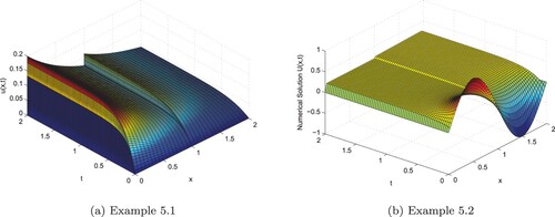
Figure 2. Solution profile for different time level at $ϵ={10}^{-3}$ and $N=32,\mathrm{\Delta }t=\frac{0.1}{2^2}$. (a) Example 5.1 and (b) Example 5.2.

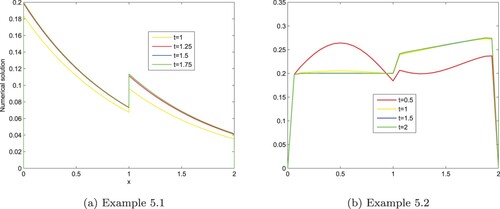
Figure 3. ε-uniform convergence in Log–Log scale for different values of ε. (a) Example 5.1 and (b) Example 5.2.

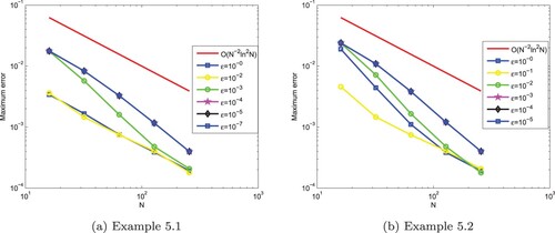
Table 1. Maximum pointwise errors ($E_{ϵ}^{N,\mathrm{\Delta }t}$) and rate of convergence (${\rho }^{N,\mathrm{\Delta }t}$) for Example  5.1 at different values of N and $\mathrm{\Delta }t$ for ${\lambda }_1=1/6,{\lambda }_2=1/3$.

ε	N = 16	N = 32	N = 64	N = 128	N = 256
↓	$\mathrm{\Delta }t=\frac{0.1}{2}$	$\mathrm{\Delta }t=\frac{0.1}{2^2}$	$\mathrm{\Delta }t=\frac{0.1}{2^3}$	$\mathrm{\Delta }t=\frac{0.1}{2^4}$	$\mathrm{\Delta }t=\frac{0.1}{2^5}$
${10}^{-0}$	3.4236e–03	1.6641e–03	7.5476e–04	3.9017e–04	1.9242e–04
${10}^{-1}$	3.6272e–03	1.4595e–03	7.4795e–04	4.0706e–04	2.0804e–04
${10}^{-2}$	1.7607e–02	5.7390e–03	1.6026e–03	4.7976e–04	1.7928e–04
${10}^{-3}$	1.7695e–02	8.3101e–03	3.2805e–03	1.1664e–03	3.9876e–04
${10}^{-4}$	1.7721e–02	8.3104e–03	3.2805e–03	1.1664e–03	3.9876e–04
${10}^{-5}$	1.7728e–02	8.3106e–03	3.2805e–03	1.1664e–03	3.9876e–04
${10}^{-6}$	1.7731e–02	8.3107e–03	3.2805e–03	1.1664e–03	3.9876e–04
${10}^{-7}$	1.7731e–02	8.3107e–03	3.2805e–03	1.1664e–03	3.9876e–04
${10}^{-8}$	1.7732e–02	8.3108e–03	3.2805e–03	1.1664e–03	3.9876e–04
${10}^{-9}$	1.7732e–02	8.3108e–03	3.2805e–03	1.1664e–03	3.9876e–04
${10}^{-10}$	1.7732e–02	8.3108e–03	3.2805e–03	1.1664e–03	3.9876e–04
$E^{N,\mathrm{\Delta }t}$	1.7732e–02	8.3108e–03	3.2805e–03	1.1664e–03	3.9876e–04
${\rho }^{N,\mathrm{\Delta }t}$	1.0933e+00	1.3411e+00	1.4919e+00	1.5485e+00	–

Table 2. Comparison of $ϵ-$uniform error $\left(E^{N,\mathrm{\Delta }t}\right)$ and $ϵ-$uniform rate of convergence $\left({\rho }^{N,\mathrm{\Delta }t}\right)$ of the proposed scheme for Example  5.1 and results in  [29].

ε	N = 164	N = 32	N = 64	N = 128	N = 256
↓	$\mathrm{\Delta }t=\frac{0.1}{2}$	$\mathrm{\Delta }t=\frac{0.1}{2^2}$	$\mathrm{\Delta }t=\frac{0.1}{2^3}$	$\mathrm{\Delta }t=\frac{0.1}{2^4}$	$\mathrm{\Delta }t=\frac{0.1}{2^5}$
Proposed method
$E^{N,\mathrm{\Delta }t}$	1.7732e–02	8.3108e–03	3.2805e–03	1.1664e–03	3.9876e–04
${\rho }^{N,\mathrm{\Delta }t}$	1.0933e+00	1.3411e+00	1.4919e+00	1.5485e+00	–
Result in  [29]
$E^{N,\mathrm{\Delta }t}$	2.0615e–02	1.2534e–02	6.9738e–03	3.6873e–03	1.8972e–03
${\rho }^{N,\mathrm{\Delta }t}$	7.1783e–01	8.4584e–01	9.1937e–01	9.5873e–01	–

Table 3. Maximum pointwise errors ($E_{ϵ}^{N,\mathrm{\Delta }t}$) and rate of convergence (${\rho }^{N,\mathrm{\Delta }t}$) for Example  5.2 at different values of N and $\mathrm{\Delta }t$ for ${\lambda }_1=1/6,{\lambda }_2=1/3$.

ε	N = 16	N = 32	N = 64	N = 128	N = 256
↓	$\mathrm{\Delta }t=\frac{0.1}{2}$	$\mathrm{\Delta }t=\frac{0.1}{2^2}$	$\mathrm{\Delta }t=\frac{0.1}{2^3}$	$\mathrm{\Delta }t=\frac{0.1}{2^4}$	$\mathrm{\Delta }t=\frac{0.1}{2^5}$
${10}^{-0}$	1.9025e–02	4.4272e–03	1.1083e–03	3.8543e–04	1.9205e–04
${10}^{-1}$	4.5900e–03	1.4646e–03	7.4518e–04	4.0692e–04	2.0804e–04
${10}^{-2}$	2.3879e–02	7.1708e–03	1.6581e–03	4.7968e–04	1.7928e–04
${10}^{-3}$	2.3963e–02	1.0918e–02	3.8406e–03	1.2093e–03	4.0191e–04
${10}^{-4}$	2.3990e–02	1.0925e–02	3.8433e–03	1.2099e–03	4.0191e–04
${10}^{-5}$	2.3998e–02	1.0927e–02	3.8440e–03	1.2099e–03	4.0191e–04
${10}^{-6}$	2.4000e–02	1.0927e–02	3.8442e–03	1.2099e–03	4.0191e–04
${10}^{-7}$	2.4001e–02	1.0928e–02	3.8442e–03	1.2099e–03	4.0191e–04
${10}^{-8}$	2.4001e–02	1.0928e–02	3.8443e–03	1.2099e–03	4.0191e–04
${10}^{-9}$	2.4001e–02	1.0928e–02	3.8443e–03	1.2099e–03	4.0191e–04
${10}^{-10}$	2.4001e–02	1.0928e–02	3.8443e–03	1.2099e–03	4.0191e–04
$E^{N,\mathrm{\Delta }t}$	2.4001e–02	1.0928e–02	3.8443e–03	1.2099e–03	4.0191e–04
${\rho }^{N,\mathrm{\Delta }t}$	1.1351e+00	1.5072e+00	1.6678e+00	1.5899e+00	–

Table 4. Comparison of $ϵ-$uniform error $\left(E^{N,\mathrm{\Delta }t}\right)$ and ε-uniform rate of convergence $\left({\rho }^{N,\mathrm{\Delta }t}\right)$ of the proposed scheme for Example  5.2 and results in  [29].

ε	N = 16	N = 32	N = 64	N = 128	N = 256
↓	$\mathrm{\Delta }t=\frac{0.1}{2}$	$\mathrm{\Delta }t=\frac{0.1}{2^2}$	$\mathrm{\Delta }t=\frac{0.1}{2^3}$	$\mathrm{\Delta }t=\frac{0.1}{2^4}$	$\mathrm{\Delta }t=\frac{0.1}{2^5}$
Proposed method
$E^{N,\mathrm{\Delta }t}$	2.4001e–02	1.0928e–02	3.8443e–03	1.2099e–03	4.0191e–04
${\rho }^{N,\mathrm{\Delta }t}$	1.1351e+00	1.5072e+00	1.6678e+00	1.5899e+00	–
Result in  [29]
$E^{N,\mathrm{\Delta }t}$	1.8765e–01	1.4776e–01	9.7571e–02	5.7092e–02	3.1057e–02
${\rho }^{N,\mathrm{\Delta }t}$	3.4479e–01	5.9873e–01	7.7316e–01	8.7837e–01	–

Acknowledgments

The authors are thankful to the anonymous reviewers for their careful reading of our manuscript and their valuable comments/suggestions which improved the organization and the quality of the work.

Disclosure statement

No potential conflict of interest was reported by the author(s).

References

- Wang XT. Numerical solution of delay systems containing inverse time by hybrid functions. Appl Math Comput. 2006;173:535–546. doi: 10.1016/j.amc.2005.04.056
- Roos HG, Stynes M, Tobiska L. Numerical methods for singularly perturbed differential equations: convection–diffusion and flow problems. New York: Springer; 1996.
- McCartin BJ. Discretization of the semiconductor device equations. In: Miller JJH, editor. New Problems and New Solutions for Device and Process Modelling. Dublin: Boole Press; 1985.
- Glizer VY. Asymptotic solution of a boundary-value problem for linear singularly perturbed functional differential equations arising in optimal control theory, J. Optim Theory Appl. 2000;106:309–335. doi: 10.1023/A:1004651430364
- Stein RB. Some models of neuronal variability. Biophys J. 1967;7:37–68. doi: 10.1016/S0006-3495(67)86574-3
- Wu J. Theory and applications of partial functional differential equations. New York: Springer; 1996.
- Kuang Y. Delay differential equations with applications in population dynamics. New York: Academic Press; 1993.
- Ramesh V, Kadalbajoo MK. Upwind and midpoint upwind difference methods for time-dependent differential difference equations with layer behavior. Appl Math Comput. 2008;202:453–471. doi: 10.1016/j.amc.2007.11.033
- Kumar D. An implicit scheme for singularly perturbed parabolic problem with retarded terms arising in computational neuroscience. Numer Methods Partial Differ Equ. 2018;34:1933–1952. doi: 10.1002/num.v34.6
- Ramesh V, Priyanga B. Higher order uniformly convergent numerical algorithm for time-dependent singularly perturbed differential-difference equations. Differ Equ Dyn Syst. 2021;29:239–263. doi: 10.1007/s12591-019-00452-4
- Woldaregay MM, Duressa GF. Parameter uniform numerical method for singularly perturbed parabolic differential difference equations. J Niger Math Soc. 2019;38:223–245. https://ojs.ictp.it/jnms/.
- Ejere AH, Woldaregay MM. A uniformly convergent numerical scheme for solving singularly perturbed differential equations with large spatial delay. SN Applied Sciences; Published online 2022. doi: 10.1007/s42452-022-05203-9
- Bansal K, Sharma KK. Numerical treatment for the class of time dependent singularly perturbed parabolic problems with general shift arguments. Differ Equ Dyn Syst. 2017;25:327–346. doi: 10.1007/s12591-015-0265-7
- Rao RN, Chakravarthy PP. Fitted numerical methods for singularly perturbed one dimensional parabolic partial differential equations with small shifts arising in the modelling of neuronal variability. Differ Equ Dyn Syst. 2019;27:1–18. doi: 10.1007/s12591-017-0363-9
- Debela HG, Duressa GF. Accelerated fitted operator finite difference method for singularly perturbed delay differential equations with non-local boundary condition. J Egypt Math Soc. 2020;28(1):1–16. doi: 10.1186/s42787-020-00076-6
- Sekar E, Tamilselvan A. Singularly perturbed delay differential equations of convection–diffusion type with integral boundary condition. J Appl Math Comput. 2019;59(1-2):701–722. doi: 10.1007/s12190-018-1198-4
- Debela HG, Duressa GF. Exponentially fitted finite difference method for singularly perturbed delay differential equations with integral boundary condition. Int J Eng Appl Sci. 2019;11(4):476–493. doi: 10.24107/ijeas.647640
- Cimen E, Cakir M. Convergence analysis of finite difference method for singularly perturbed non-local differential difference problem. Miskolc Math Notes. 2018;19(2):795–812. doi: 10.18514/MMN.2018.2302
- Cimen E. Numerical solution of a boundary value problem including both delay and boundary layer. Math Model Anal. 2018;23(4):568–581. doi: 10.3846/mma.2018.034
- Cimen E, Amiraliyev GM. Uniform convergence method for a delay differential problem with layer behaviour. Mediterr J Math. 2019;16:57. doi: 10.1007/s00009-019-1335-9
- Das P. Comparison of a priori and a posteriori meshes for singularly perturbed nonlinear parameterized problem. J Comput Appl Math. 2015;290:16–25. doi: 10.1016/j.cam.2015.04.034
- Das P, Vigo-Aguiar J. Parameter uniform optimal order numerical approximation of a class of singularly perturbed system of reaction diffusion problems involving a small perturbation parameter. J Comput Appl Math. 2017;354:533–544. doi: 10.1016/j.cam.2017.11.026
- Das P, Rana S, Vigo-Aguiar J. Higher order accurate approximations on equidistributed meshes for boundary layer originated mixed type reaction diffusion systems with multiple scale nature. Appl Numer Math. 2020;148:79–97. doi: 10.1016/j.apnum.2019.08.028
- Das P,Natesan S. A uniformly convergent hybrid scheme for singularly perturbed system of reaction–diffusion Robin type boundary-value problems. J Appl Math Comput. 2013;41:447–471. doi: 10.1007/s12190-012-0611-7
- Das P, Natesan S. Higher-order parameter uniform convergent schemes for robin type reaction diffusion problems using adaptively generated grid. Int J Comput Methods. 2012;9(4):1250052 (27 pages). doi: 10.1142/S0219876212500521.
- Chandru M, Das P, Ramos H. Numerical treatment of two-parameter singularly perturbed parabolic convection diffusion problems with non-smooth data. Math Meth Appl Sci. 2018;41(14):1–29. doi: 10.1002/mma.5067
- Kumar D, Kumari P. Parameter-uniform numerical treatment of singularly perturbed initial-boundary value problems with large delay. Appl Numer Math. 2020, July;153:412–429. doi: 10.1016/j.apnum.2020.02.021
- Bahuguna D, Dabas J. Existence and uniqueness of a solution to a semilinear partial delay differential equation with an integral condition. Nonlinear Dyn Syst Theory. 2008;8(1):7–19.
- Elango S, Tamilselvan A, Vadivel R, et al. Finite difference scheme for singularly perturbed reaction diffusion problem of partial delay differential equation with nonlocal boundary condition. Adv Differ Equ. 2021;2021:151. doi: 10.1186/s13662-021-03296-x
- Gobena WT, Duressa GF. Parameter-Uniform numerical scheme for singularly perturbed delay parabolic reaction diffusion equations with integral boundary condition. Int J Differ Equ. 2021;2021:Article ID 9993644, 16 pages. doi: 10.1155/2021/9993644
- Gobena WT, Duressa GF. Exponentially fitted robust scheme for the solution of singularly perturbed delay parabolic differential equations with integral boundary condition. (preprint). doi: 10.21203/rs.3.rs-2081265/v1
- Gobena WT, Duressa GF. Parameter uniform numerical methods for singularly perturbed delay parabolic differential equations with non-local boundary condition. Int J Eng Sci Technol. 2021;13(2):57–71. doi: 10.4314/ijest.v13i2.7.
- Gobena WT, Duressa GF. Fitted Operator Average Finite Difference Method for Singularly Perturbed Delay Parabolic Reaction Diffusion Problems with Non-Local Boundary Conditions. Tamkang Journal of Mathematics; Article in press. doi: 10.5556/j.tkjm.54.2023.4175
- Gobena WT, Duressa GF. An optimal fitted numerical scheme for solving singularly perturbed parabolic problems with large negative shift and integral boundary condition. Results Control Optim. 2022;100172:1–15. Article in press. doi: 10.1016/j.rico.2022.100172
- Ladyzhenskaya OA, Solonnikov VA, Ural'tseva NN. Linear and quasi-linear equations of parabolic type. USA: American Mathematical Society; 1968. (Translations of Mathematical Monographs; Vol. 23).
- Kadalbajoo MK, Awasthi A. The midpoint upwind finite difference scheme for time-dependent singularly perturbed convection–diffusion equations on non-uniform mesh. Int J Comput Methods Eng Sci Mech. 2011;12(3):150–159. doi: 10.1080/15502287.2011.564264
- Roos HG, Stynes M, Tobiska L. Robust numerical methods for singularly perturbed differential equations: convection–diusion–reaction and flow problems. Berlin Heidelberg; 2008. (Springer Science and Business Media; 24).
- Clavero C, Gracia JL. On the uniform convergence of a finite difference scheme for time dependent singularly perturbed reaction–diffusion problems. Appl Math Comput. 2010;216(5):1478–1488. doi: 10.1016/j.amc.2010.02.050
- Aziz T, Khan A, Khan I, et al. A variable-mesh approximation method for singularly perturbed boundary-value problems using cubic spline in tension. Int J Comput Math. 2004;81:1513–1518. doi: 10.1080/00207160412331284169