A hybrid method for an inverse scattering problem related to cylindrical bodies buried in a half-space

Abstract

A hybrid method which is suitable to find numerical solutions for two-dimensional inverse scattering problems connected with cylindrical bodies buried in a half-space with the known orientation is established. The mentioned hybrid method is based on the classical moment method in connection with vertical coordinate while it involves the horizontal coordinate through a spectral expansion. The structure of the spectral expansion which is imposed by the Green's function contributes to improvement of the ill-posedness of the problem along with Tikhonov regularization. By taking this particular structure into consideration one determines the basis functions such that the effect of the ill-posedness is reduced to a minimum. Some illustrative examples show the applicability and accuracy of the method.

KEYWORDS:

• Inverse scattering
• Buried cylindrical body
• Basis functions
• Tikhonov regularization
• Ill-posedness

1. Introduction

Inverse scattering problems whose main aim is to recover the geometrical as well as the physical properties of an inaccessible body by considering its effect on the propagation of certain waves have been extensively studied. By geometrical properties, one refers to the shape and location of the body while by physical properties its constitutive parameters. The principal reason for this excessive interest in inverse scattering problems is their direct application in certain domain of great practical importance such as medical diagnosis, geophysical prospecting, nondestructive probing, telecommunication, astronomical researches, determination of underground tunnels and pipelines, underwater observations etc. A great deal of the available investigations concern the case where the body is located in an infinite homogeneous space. For this simplest and rather idealized case several exact [1–6], approximate [3,6–8] and direct numerical solution techniques [9–22] have been established. In contrast to a huge number of studies for the inverse problems with homogeneous host medium, the investigations related to the case where the body is buried in a known limited host medium are less than those of homogeneous medium. A reason for this scarcity is, of course, the mathematical difficulties due to the complicated behaviour of the total field inside the host medium. Because of these difficulties, as far as we know, there is a limited number of investigations which are based on purely exact or purely numerical methods in the open literature. All of the well-known studies concerning this case depend generally on RF Tomography [23–29] and Born, Rytov or other kind of approximations [30–41]. Mathematical difficulties to establish exact or numerical techniques for buried objects can be divided into two groups as follows:

1. The ill-posedness of the problem,

2. The non-existence of an explicit expression of the related Green's function suitable for numerical implementations.

The ill-posedness which is a characteristic feature of such inverse problems, proceeds from the fact that the related direct problem is based on a compact operator [3]. As we shall explain below, this fact can also be seen from the spectral structure which consists of some transforms (Fourier, Laplace, Kontorovich-Lebedev, etc.) or series expansions of the related Green's function for inhomogeneous spaces. For the case to be treated in the present paper, in which the mediums containing and not containing buried body become two different simple half-spaces having the wave-numbers and $k_0$, respectively, the spectral representation of the Green's function involves a factor of the form $\exp \left\{-\sqrt{v^2-k_0^2}{x}_2+\sqrt{v^2-k_1^2}{y}_2\right\}$ where $v\in \mathbb{R}$, $x_2>0$, $y_2<0$ and $k_1>k_0$ [36]. This factor obviously causes evanescent waves when $|v|>k_0$. In the numerical solution of the direct problem, this factor plays a helpful role and enables one to truncate the inverse transform integral for $|v|>k_0$. Conversely, in the inverse problem it acts as $\exp \left\{\sqrt{v^2-k_0^2}{x}_2-\sqrt{v^2-k_1^2}{y}_2\right\}$ and obviously can have considerable effects on the solution. This point explains the ill-posed behaviour of the inverse problem. In order to reduce the distributing effect of evanescent waves in the inverse problem we shall try to establish a ‘hybrid method’ in which the above-mentioned spectral representation takes place directly so that a truncation in the domain $|v|>k_0$ is plausible. To this end we will choose the basis functions such that they have bounded supports and minimum valued spectral duration.

In this work, since the orientation related to buried bodies which consist of an infinitely long cylinder with arbitrary cross-section has already been determined by using a Born approximation-based technique explained in [35] and also [30], we only focused on the development of a hybrid method which will uncover the constitutive parameters and the geometry of the cross-section of the cylindrical buried body. Herein the essential reason to consider the two-dimensional infinitely long cylindrical bodies is that in the most of practical applications citied above the buried bodies are generally homogeneous along their main axes and maximumly have two-dimensional constitutive parameters variation on their cross-sections. And also, beside this when the wave length related to the illuminating source is chosen sufficiently small as compared with the lengths of axes of the buried bodies then the problem can easily be assumed to be in the form described in this study. This is also worthwhile to point out that this kind of assumption provides remarkable simplicities for the solution of the problem in mathematical point of views. The results obtain in [28], where a certain configuration of a wideband (3–6 GHz) multi-antenna microwave tomography system assumes that both imaging target and wave field propagation are in two dimension, exhibit the relevance and as well as reliability for the consideration of the two-dimensional buried cylindrical body problem. For this purpose, in Section 2 the problem is reduced to the solution of an integral equation involving the Fourier transform of the Green's function. The essential points of the method as well as determination of the basis functions will be explained in Section 3. In Section 4 effectiveness of the method is also shown by presenting some illustrative examples. Finally, some concluding remarks are given in Section 5.

The notation to be used in the paper is the usual standard one where $x=(x_1,x_2,x_3)\in {\mathbb{R}}^3$shows both the point $x$ with Cartesian coordinates $(x_1,x_2,x_3)$ and the position vector having the same components. The projection of $x$ on the plane $x_3=0$ will be indicated by $x^{\mathrm{\prime }}=(x_1,x_2)\in {\mathbb{R}}^2$. Finally, a time factor $\exp \left\{-i\omega t\right\}$will be assumed and omitted throughout the paper.

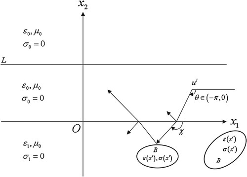
2. Formulation of the problem

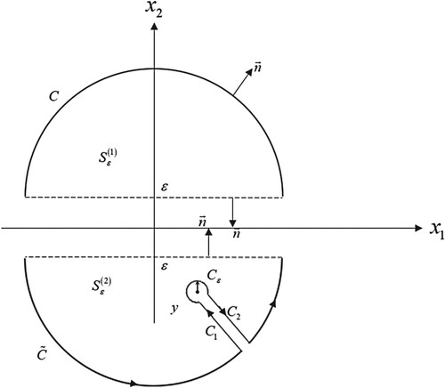
Let the half-spaces $x_2>0$ and $x_2<0$ be filled with simple non-conducting and non-magnetic materials having different permittivity ${ϵ}_0$ and ${ϵ}_1$, respectively. We assume that the region $x_2<0$ involves a non-magnetic cylindrical body $D$ whose permittivity $ϵ\left(x^{\mathrm{\prime }}\right)$ and conductivity $\sigma \left(x^{\mathrm{\prime }}\right)$ are unknown bounded functions of $x^{\mathrm{\prime }}=(x_1,x_2)$. The cross-section of $D$, say $B$, can be composed of several disconnected regions (see Figure 1). The problem to be considered here consists of the determination of the functions $ϵ\left(x^{\mathrm{\prime }}\right)$ and $\sigma \left(x^{\mathrm{\prime }}\right)$ by using the data collected by measurements in the half-space $x_2>0$, more precisely: on the line $L=\left\{x|x_1\in \left(-\mathrm{\infty },\mathrm{\infty }\right),x_2=constant>0,x_3=0\right\}$. To this end we illuminate the body by a linearly polarized monochromatic plane wave whose electric field is chosen to be parallel to the orientation of the cylindrical body that is known beforehand, i.e.: (1) $E=\left(0,0,u^i\left(x^{\mathrm{\prime }}\right)\right)$(1) with (2) $u^i\left(x^{\mathrm{\prime }}\right)=e^{i{k}_0\left(x_1\cos \theta +x_2\sin \theta \right)},\theta \in \left(-\pi ,0\right),$(2) where $k_0=\omega \sqrt{{ϵ}_0{\mu }_0}$ stands for the wave number in the above half-space. In what follows we suppose that the wave number in the lower half-space, say $k_1=\omega \sqrt{{ϵ}_1{\mu }_0}$, is greater than $k_0$.

Figure 1. Geometry of the problem.

In order to formulate the problem easily, let us introduce $u_0\left(x^{\mathrm{\prime }}\right)$ which can be defined as the total field when the body $D$ is absent. As it is well-known the expression of this field is given: (3) $u_0\left(x^{\mathrm{\prime }}\right)=\{\begin{array}{l}{u}^i+R{e}^{i{k}_0\left(x_1\cos \theta -x_2\sin \theta \right)},x_2>0\\ T{e}^{i{k}_1\left(x_1\cos \chi +x_2\sin \chi \right)},x_2<0\end{array}$(3) where $R$ and $T$ show the reflection and transmission coefficients, respectively, namely: (4) $R=\frac{k_0\sin \theta -k_1\sin \chi }{k_0\sin \theta +k_1\sin \chi }$(4) and (5) $T=\frac{2k_0\sin \theta }{k_0\sin \theta +k_1\sin \chi }$(5) while $\chi$ stands for the transmission angle satisfying the Snell’s law: (6) $\cos \chi =\frac{k_0}{k_1}\cos \theta ,\chi \in \left(-\pi ,0\right).$(6) As it is well-known, $u_0\left(x^{\mathrm{\prime }}\right)$ satisfies the Helmholtz equation. (7) $\Delta u_0+k^2\left(x_2\right)u_0=0$(7) in the sense of distribution, which implicitly involves the boundary conditions too [37]. Here $k\left(x_2\right)$ shows the wave number of the two-part space, namely: (8) $k\left(x_2\right)=\{\begin{array}{l}{k}_0,x_2>0\\ k_1,x_2<0.\end{array}$(8) The contribution of the body $D$ to the total field $u\left(x^{\mathrm{\prime }}\right)$, say $u_D\left(x^{\mathrm{\prime }}\right)$ which can be defined by. (9) $u_D\left(x^{\mathrm{\prime }}\right)=u\left(x^{\mathrm{\prime }}\right)-u_0\left(x^{\mathrm{\prime }}\right)$(9) satisfies the equation (10) $\Delta u_D+k^2\left(x_2\right)u_D=-k_1^2\upsilon \left(x^{\mathrm{\prime }}\right)u\left(x^{\mathrm{\prime }}\right)$(10) in the sense of distribution [36] under the Sommerfeld radiation condition. (11) $\sqrt{|x^{\mathrm{\prime }}|}\left\{\frac{\mathrm{\partial }}{\mathrm{\partial }|x^{\mathrm{\prime }}|}{u}_D-ik{u}_D\right\}\to Oas|x^{\mathrm{\prime }}|\to \mathrm{\infty }.$(11) In (10) $\upsilon \left(x^{\mathrm{\prime }}\right)$ has the following significance: (12) $\upsilon \left(x^{\mathrm{\prime }}\right)=\frac{{ϵ}^{\mathrm{\prime }}\left(x^{\mathrm{\prime }}\right)}{ϵ\left(x_2\right)}-1$(12) where (13) ${ϵ}^{\mathrm{\prime }}\left(x^{\mathrm{\prime }}\right)=ϵ\left(x^{\mathrm{\prime }}\right)+\frac{i\sigma \left(x^{\mathrm{\prime }}\right)}{\omega }$(13) and (14) $ϵ\left(x_2\right)=\{\begin{array}{l}{ϵ}_0,x_2>0\\ {ϵ}_1,x_2<0.\end{array}$(14) It is evident that outside $B$ ${ϵ}^{\mathrm{\prime }}\left(x^{\mathrm{\prime }}\right)$ is identical with $ϵ\left(x_2\right)$, then the object function $\upsilon \left(x^{\mathrm{\prime }}\right)$ becomes zero. This means that the determination of $\upsilon \left(x^{\mathrm{\prime }}\right)$ is sufficient to solve the problem completely because its support describes the region $B$ while its real and imaginary parts permit one to find the permittivity $ϵ\left(x^{\mathrm{\prime }}\right)$ and the conductivity $\sigma \left(x^{\mathrm{\prime }}\right)$ of the buried body $D$, respectively. Hence the problem consists in determining the function $\upsilon \left(x^{\mathrm{\prime }}\right)\in {\mathit{\text{L}}}_{\mathrm{\infty }}\left(B\right)$ appearing in (10) by using the measured values of $u_D\left(x^{\mathrm{\prime }}\right)$ on the afore-mentioned data line $\text{L}$. In order to solve this problem, we will first derive an integral equation which is equivalent to (10) and (11).

2.1. An equivalent integral equation

It is well-known that the Green’s function of the two-part space not involving the buried body $D$, say $G_0\left(x^{\mathrm{\prime }},y^{\mathrm{\prime }}\right)$, satisfies the equation (15) $\Delta G_0\left(x^{\mathrm{\prime }},y^{\mathrm{\prime }}\right)+k^2\left(x_2\right)G_0\left(x^{\mathrm{\prime }},y^{\mathrm{\prime }}\right)=-\delta \left(x_1-y_1\right)\delta \left(x_2-y_2\right),y_2<0$(15) in the sense of distribution under the Sommerfeld radiation condition. For the sake of simplicity and legibility of the paper, an explicit expression of $G_0\left(x^{\mathrm{\prime }},y^{\mathrm{\prime }}\right)$ will be derived later. By considering the fact that (10) and (15) are valid in the sense of distributions and repeating the well-known classical procedure which is based on Stokes’ theorem (see Appendix A), one obtains the integral equation (16) $u_D\left(x^{\mathrm{\prime }}\right)=k_1^2{\int }_B{G}_0\left(x^{\mathrm{\prime }},y^{\mathrm{\prime }}\right)\upsilon \left(y^{\mathrm{\prime }}\right)u\left(y^{\mathrm{\prime }}\right)d{y}^{\mathrm{\prime }}$(16) that will be used for the solution of the problem. Since $\upsilon \left(y^{\mathrm{\prime }}\right)$ appearing in (16) is naught outside $B$, the last integral equation can also be written as follows: (17) $u_D\left(x^{\mathrm{\prime }}\right)=k_1^2{\int }_{{\mathbb{R}}^2}{G}_0\left(x^{\mathrm{\prime }},y^{\mathrm{\prime }}\right)\upsilon \left(y^{\mathrm{\prime }}\right)u\left(y^{\mathrm{\prime }}\right)d{y}^{\mathrm{\prime }}.$(17) Let us now obtain an explicit expression of $G_0\left(x^{\mathrm{\prime }},y^{\mathrm{\prime }}\right)$ for $x_2>0$ where the measurements will be realized and $y_2<0$. For this purpose, by assuming that $k_0$ has a small positive imaginary part, we consider first the Fourier transform of $G_0$ with respect to $x_1$, namely: (18) ${\hat{G}}_0\left(v,x_2,y^{\mathrm{\prime }}\right)={\int }_{-\mathrm{\infty }}^{\mathrm{\infty }}{G}_0\left(x_1,x_2,y^{\mathrm{\prime }}\right)e^{-iv{x}_1}d{x}_1.$(18) Owing to the radiation condition to which $G_0$ is subjected one has. (19) $G_0\left(x^{\mathrm{\prime }},y^{\mathrm{\prime }}\right)\sim A{e}^{i{k}_0|x_1|}/\sqrt{|x_1|}\text{as }{x}_1\to \pm \mathrm{\infty },x_2=constant>0.$(19) From (19) it is evident that the function ${\hat{G}}_0$ is regular in the strip (20) $-\mathrm{\Im }{k}_0<\mathrm{\Im }v<\mathrm{\Im }{k}_0$(20) where $\mathrm{\Im }{k}_0$ stands for imaginary part of $k_0$. 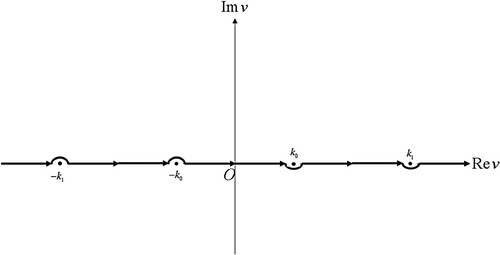If one makes now $\mathrm{\Im }{k}_0\to +0$, then the above-mentioned regularity strip degenerates to the real axis intended at $\pm k_0$ and $\pm k_1$ as shown in Figure 2. This intended line will be denoted by $\mathcal{L}$.

Figure 2. The degenerated regularity strip and branch cut in the complex $v$-plane.

By taking the Fourier transform of (15) with respect to $x_1$ it is an easy matter to show that ${\hat{G}}_0$ satisfies the equation. (21) $\frac{{\mathrm{\partial }}^2}{\mathrm{\partial }{x}_2^2}{\hat{G}}_0-\left[v^2-k^2\left(x_2\right)\right]{\hat{G}}_0=-e^{-iv{y}_1}\delta \left(x_2-y_2\right)$(21) which yields (22) ${\hat{G}}_0\left(v,x_2,y^{\mathrm{\prime }}\right)=\frac{1}{\alpha \left(v\right)+\text{β}\left(v\right)}{e}^{-iv{y}_1+\text{β}\left(v\right)y_2-\alpha \left(v\right)x_2},x_2>0,y_2<0$(22) with (23) $\alpha \left(v\right)=\sqrt{v^2-k_0^2},\text{β}\left(v\right)=\sqrt{v^2-k_1^2}.$(23) Here the square-root functions are defined in the $v$-plane cut along the real axis from $\left(-\mathrm{\infty };-k_0,-k_1\right)$ and $\left(k_0,k_1;\mathrm{\infty }\right)$ as shown in Figure 2 with the conditions $\alpha \left(0\right)=-i{k}_0,\text{β}\left(0\right)=-i{k}_1$. Therefore, the explicit expression for the Green’s function in the region where $x_2>0$ while $y_2<0$ can be obtained by considering the inverse Fourier transform of (22) which is written by (24) $G_0\left(x_1,x_2,y_1,y_2\right)=\frac{1}{2\pi }{\int }_{\mathcal{L}}{\hat{G}}_0\left(v,x_2,y^{\mathrm{\prime }}\right)e^{iv{x}_1}dv=\frac{1}{2\pi }{\int }_{\mathcal{L}}\frac{e^{iv\left(x_1-y_1\right)+\text{β}\left(v\right)y_2-\alpha \left(v\right)x_2}}{\alpha \left(v\right)+\text{β}\left(v\right)}dv.$(24) From (24) we conclude that the Green’s function $G_0\left(x_1,x_2,y_1,y_2\right)$ depends only on the difference $\left(x_1-y_1\right)$ as a function of $x_1$ and $y_1$. This shows that the first integration with respect to $y_1$ appearing in (17) is a convolution on $x_1$. By considering this fact the equation (17) and its Fourier transformation with respect to $x_1$ can be written as. (25) $u_D\left(x_1,x_2\right)=k_1^2{\int }_{-\mathrm{\infty }}^{\mathrm{\infty }}{G}_0\left(x_1,x_2,0,y_2\right)\ast \left[\upsilon \left(x_1,y_2\right)u\left(x_1,y_2\right)\right]d{y}_2$(25) and (26) ${\hat{u}}_D\left(v,x_2\right)=k_1^2{\int }_{-\mathrm{\infty }}^{\mathrm{\infty }}{\hat{G}}_0\left(v,x_2,0,y_2\right)\hat{p}\left(v,y_2\right)d{y}_2$(26) respectively. In (26) $\hat{p}\left(v,y_2\right)$ is the Fourier transform of (27) $p\left(y^{\mathrm{\prime }}\right)=\upsilon \left(y^{\mathrm{\prime }}\right)u\left(y^{\mathrm{\prime }}\right)$(27) given by (28) $\hat{p}\left(v,y_2\right)={\int }_{-\mathrm{\infty }}^{\mathrm{\infty }}p\left(y_1,y_2\right)e^{-iv{y}_1}d{y}_1.$(28) Since the inverse Fourier transform applied to (26) will result in much more complicated expressions that can be easily checked from (24) and (25), the method to be established in this work will be based on the equation (26) itself rather than (16) or (25). The essential points of the method will be explained in the next section.

3. A hybrid method for numerical solution

From (22-24) and (26) it is an easy matter to conclude that the contribution from the portion $k_0<|v|<\mathrm{\infty }$ of $\mathcal{L}$ to the field consists of a composition of evanescent waves. Hence, in the numerical computation of the field where the direct problem is in question this contribution can be neglected. But the situation is quite converse in the case of inverse problems. Indeed, in the solution of the inverse problem the above-mentioned evanescent terms act as exponentially growing terms and thus yield the ill-posedness of the inverse problem as explained more explicitly in Section 1. In what follows one will try to remove this effect.

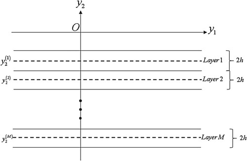
Consider now $M$layers, each with a thickness of $2h$ in the host half-space such that the region $B$ is supposed to be completely covered by these layers (see Figure 3). The thickness $2h$ mentioned above is so chosen that the variation of $p\left(y_1,y_2\right)$ as a function of $y_2$ can be neglected inside each layer. Then for the dependence on the horizontal coordinate $y_1$ we consider an expansion of the form. (29) $p\left(y_1,y_2^{\left(m\right)}\right)=\sum _{n=-N}^N{A}_{mn}{\varphi }_n\left(y_1\right),m=1,2,3,\dots ,M$(29) where ${\varphi }_n\left(y_1\right)$ stand for basis functions that will be determined later in Section 3.1. The expression $A_{mn}$ appearing in (29) shows the constant coefficients which are yet unknown. By considering first that the integral contribution in (26) comes from $M$ layers and then substituting $\hat{p}\left(v,y_2\right)$ which is obtained by the Fourier transform of (29) with respect to$y_1$ in (26), one gets (30) ${\hat{u}}_D\left(v,x_2\right)=k_1^2\sum _{m=1}^M\sum _{n=-N}^N{A}_{mn}{\hat{\varphi }}_n\left(v\right){\int }_{y_2^{\left(m\right)}-h}^{y_2^{\left(m\right)}+h}{\hat{G}}_0\left(v,x_2,0,y_2\right)d{y}_2.$(30) In order to determine $\left(2N+1\right)M$ unknown coefficients $A_{mn}$ mentioned above, one has to obtain a linear algebraic system of the same number of equations. To do this, let us consider (22) with $y_1=0$ in (30) and replace the Fourier transform parameter $v$ by properly chosen values $v_1,v_2,\dots ,v_{(2N+1)M}$ on both side of the equations (30) such that $v_t=-k_0+\frac{2k_0}{\left(2N+1\right)M+1}t$, for $t=1,2,\dots ,\left(2N+1\right)M$. Thus, we write. (31) $\begin{array}{rl}& \left[\begin{array}{c}\begin{array}{ccc}{Q}_{1(-N)}^1& \begin{array}{cccc}\cdots & Q_{1N}^1& \cdots & Q_{M(-N)}^1\end{array}& \begin{array}{cc}\cdots & Q_{MN}^1\end{array}\end{array}\\ \begin{array}{cccc}{Q}_{1(-N)}^2& \cdots & \begin{array}{ccc}{Q}_{1N}^2& \cdots & Q_{M(-N)}^2\end{array}& \begin{array}{cc}\cdots & Q_{MN}^2\end{array}\end{array}\\ \begin{array}{ccc}⋮& & \begin{array}{cccc}⋮& & ⋮& \begin{array}{cc}& ⋮\end{array}\end{array}\end{array}\\ \begin{array}{ccc}{Q}_{1(-N)}^t& \cdots & \begin{array}{cccc}{Q}_{1N}^t& \cdots & Q_{M(-N)}^t& \begin{array}{cc}\cdots & Q_{MN}^t\end{array}\end{array}\end{array}\\ \begin{array}{ccc}\begin{array}{c}⋮\\ ⋮\end{array}& & \begin{array}{cccc}\begin{array}{c}⋮\\ ⋮\end{array}& & \begin{array}{c}⋮\\ ⋮\end{array}& \begin{array}{cc}& \begin{array}{c}⋮\\ ⋮\end{array}\end{array}\end{array}\end{array}\\ \begin{array}{ccc}{Q}_{1(-N)}^{(2N+1)M}& \cdots & \begin{array}{cccc}{Q}_{1N}^{(2N+1)M}& \cdots & Q_{M(-N)}^{(2N+1)M}& \begin{array}{cc}\cdots & Q_{MN}^{(2N+1)M}\end{array}\end{array}\end{array}\end{array}\right]\left[\begin{array}{c}{A}_{1\left(-N\right)}\\ ⋮\\ A_{1\left(N\right)}\\ ⋮\\ A_{M\left(-N\right)}\\ ⋮\\ A_{M\left(N\right)}\end{array}\right]\\ & =\left[\begin{array}{c}{P}_1\\ P_2\\ ⋮\\ ⋮\\ P_t\\ ⋮\\ P_{\left(2N+1\right)M}\end{array}\right]\end{array}$(31) where (32) $Q_{mn}^t=k_1{\hat{\varphi }}_n\left(v_t\right){\int }_{y_2^{\left(m\right)}-h}^{y_2^{\left(m\right)}+h}{e}^{\text{β}\left(v_t\right)y_2}d{y}_2=\frac{2k_1}{\text{β}\left(v_t\right)}{e}^{\text{β}\left(v_t\right)y_2^{\left(m\right)}}Sinh\left(\text{β}\left(v_t\right)h\right){\hat{\varphi }}_n\left(v_t\right)$(32) and (33) $P_t=\frac{1}{k_1}\left[\alpha \left(v_t\right)+\text{β}\left(v_t\right)\right]e^{\alpha \left({\nu }_t\right)x_2}{\hat{u}}_D\left(v_t,x_2\right)$(33) In order to reduce the effect of the ill-posedness explained above in addition to the method given in this section, a regularized solution of the system (31) can also be considered in the sense of Tikhonov which is nothing but the solution to the following minimization problem in ${\mathbb{C}}^{(2N+1)M}$ [42], (34) $F\left(A\right)=min\left\{F\left(\tilde{A}\right)\right\}for\tilde{A}\in {\mathbb{C}}^{(2N+1)M}$(34)

Figure 3. A layered region in the lower half-space ($y_2<0$).

where $A\in {\mathbb{C}}^{(2N+1)M}$and (35) $F\left(\tilde{A}\right)=\left||P_t-\sum _{p=1}^{(2N+1)M}{Q}_p^t{\tilde{A}}_p\right|{|}_{(2N+1)M}^2+\tau ||\tilde{A}|{|}_{(2N+1)M}^2,t=1,2,\dots ,(2N+1)M$(35) Here $||.|{|}_{(2N+1)M}$ stands for the Euclidean norm in the $(2N+1)M$- dimensional space ${\mathbb{C}}^{(2N+1)M}$, namely (36) $||\tilde{A}|{|}_{(2N+1)M}={\left\{\sum _{p=1}^{{}^{(2N+1)M}}{|{\tilde{A}}_p|}^2\right\}}^{\frac{1}{2}}$(36) In (35) $\tau \in \mathbb{R}$ is the scalar regularization parameter whose value is determined by inspection. By following the procedure mentioned in detail in [42], one can easily show that the solution of the afore-mentioned minimization problem here is equivalent to that of the algebraic system given by (37) $\left(\tau I+{\overline{Q}}^{T}Q\right)\underset{\sim }{A}={\overline{Q}}^T\underset{\sim }{P}$(37) where $I$ is the $\left(2N+1\right)M$ dimensional unit matrix while $Q$, $\underset{\sim }{A}$ and $\underset{\sim }{P}$ are the square, unknown column and right-hand side column matrices appearing in (31), respectively. In (37) ${\overline{Q}}^T$signifies the matrix which is composed by the transpose of the complex conjugate of $Q$. Since the value for the regularization parameter $\tau \in \mathbb{R}$ mentioned above is inspected, it does not exist any strict rule to identify it. In this work this parameter is chosen so that each entry on the main diagonal of the matrix $\left(\tau I+{\overline{Q}}^{T}Q\right)$ is the smallest possible largest entry in its row given by (38) $\begin{array}{l}\tau =min\left\{max\left\{\left|\sum _{p=1}^{\left(2N+1\right)M}{\overline{q}}_{pi}{q}_{pj}\right|\right\}-\sum _{p=1}^{\left(2N+1\right)M}{|q_{pi}|}^2\right\},1\le i,j\le \left(2N+1\right)M;j\ne i\\ \end{array}$(38) where $q_{ij}$ for $1\le i,j\le \left(2N+1\right)M$ are the entries of the matrix $Q$.

If one solves the system (37) for $\underset{\sim }{A}$ which contains the coefficients $A_{mn}$ and inserts these obtained values.

in (29), then one gets (39) $p\left(x_1,x_2^{\left(m\right)}\right)=\sum _{n=-N}^N{A}_{mn}{\varphi }_n\left(x_1\right),m=1,\dots ,M.$(39) On the other hand, by using the same values of $A_{mn}$ and also substituting $x_2^{\left(m\right)}$ instead of $x_2$ in (30), the inverse Fourier transformation of this equation yields (40) $\begin{array}{rl}& u_D\left(x_1,x_2^{\left(m\right)}\right)\\ & =\frac{1}{2\pi }{\int }_{-\mathrm{\infty }}^{\mathrm{\infty }}{\hat{u}}_D\left(v,x_2^{\left(m\right)}\right)e^{iv{x}_1}dv\\ & =\frac{k_1^2}{2\pi }\sum _{j=1}^M\sum _{n=-N}^N{A}_{jn}{\int }_{y_2^{\left(j\right)}-h}^{y_2^{\left(j\right)}+h}{\int }_{-\mathrm{\infty }}^{+\mathrm{\infty }}{\hat{\varphi }}_n\left(v\right){\hat{G}}_0\left(v,x_2^{\left(m\right)},0,y_2\right)e^{iv{x}_1}dvd{y}_2,m=1,\dots ,M.\end{array}$(40) It is obvious from (27) and (9) that the expression of object function for each layer can be written as (41) $\upsilon \left(x_1,x_2^{\left(m\right)}\right)=\frac{p\left(x_1,x_2^{\left(m\right)}\right)}{u_0\left(x_1,x_2^{\left(m\right)}\right)+u_D\left(x_1,x_2^{\left(m\right)}\right)},m=1,\dots ,M.$(41) Therefore, the consideration of (39), (40) and (3) for $x_2<0$ in (41) will permit us to compute numerically the explicit expression of the above-mentioned object function.

It should be remarkable that in (39-41) $x_2^{\left(m\right)}<0$ hence the expression of ${\hat{G}}_0$ appearing in (40) is different from what is given in (22). Indeed, by considering the solution of (21) for $x_2<y_2<0$ and $y_2<x_2<0$ one easily obtains that. (42) ${\hat{G}}_0\left(v,x_2^{\left(m\right)},0,y_2\right)=\{\begin{array}{l}C\left(v\right)e^{\text{β}\left(v\right)x_2^{\left(m\right)}}+D\left(v\right)e^{-\text{β}\left(v\right)x_2^{\left(m\right)}},y_2<x_2^{\left(m\right)}<0\\ E\left(v\right)e^{\text{β}\left(v\right)x_2^{\left(m\right)}},x_2^{\left(m\right)}<y_2<0.\end{array}$(42) The spectral coefficients $C\left(v\right)$, $D\left(v\right)$ and $E\left(v\right)$ appearing in (42) are presented by (43) $\begin{array}{rl}C\left(v\right)& =\frac{\text{β}\left(v\right)-\alpha \left(v\right)}{2\text{β}\left(v\right)\left[\alpha \left(v\right)+\text{β}\left(v\right)\right]}{e}^{\text{β}\left(v\right)y_2}\end{array}$(43) (44) $\begin{array}{rl}D\left(v\right)& =\frac{1}{2\text{β}\left(v\right)}{e}^{\text{β}\left(v\right)y_2}\end{array}$(44) and (45) $E\left(v\right)=\frac{\text{β}\left(v\right)-\alpha \left(v\right)}{2\text{β}\left(v\right)\left[\alpha \left(v\right)+\text{β}\left(v\right)\right]}{e}^{\text{β}\left(v\right)y_2}+\frac{1}{2\text{β}\left(v\right)}{e}^{-\text{β}\left(v\right)y_2}$(45) respectively, with $\alpha \left(v\right)$ and $\text{β}\left(v\right)$ being given in (23).

3.1. A system of basis functions

As it is explained at the beginning of Section 3, the ill-posed character of the present inverse problem is closely related to the evanescent waves corresponding to the portion $k_0<|v|<\mathrm{\infty }$ of the degenerate regularity strip $\mathcal{L}$. For this purpose, in order to reduce the effect of the ill-posedness mentioned above it is convenient to choose the values of $v_t$ related to (31) as being $|v_t|\le k_0$ where this values totally remain out of the portion $k_0<|v|<\mathrm{\infty }$. But it must be careful that to make this kind of a choice can cause some big and harmful errors when the functions corresponding to the both side of (31) are those of with wide spectrum. Because the coefficients $A_{mn}$ appearing in (30) should be determined as they also satisfy (16) which is the origin of (30) for $x_1\in \mathbb{R}$. Consequently, this situation requires that (26) or more precisely (30) should be satisfied for every $v\in \mathcal{L}$. According to the well-known concepts of the spectral estimation theory [43–44] if the Fourier transforms for the functions occurring in the above-mentioned equations have the limited duration then to perform on the computations by only considering the finite part $|v|\le k_0$ of the strip $\mathcal{L}$ gives rather good results. Hence a most plausible method for the numerical (approximate) solution of the inverse problem presented in this work will be considered as the filtration of the portion $k_0<|v|<\mathrm{\infty }$ of the line $\mathcal{L}$ by a suitable choice of the basis functions ${\varphi }_n\left(x_1\right)$. In what follows, we will show that such a choice is always possible through functions of bounded support and bounded duration.

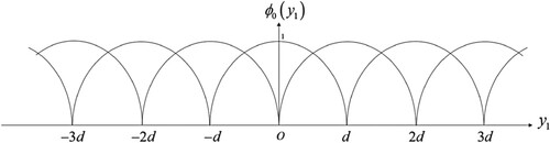
For this purpose, let us consider first the function ${\varphi }_0\left(x_1\right)$ having the support $\left(-d,d\right)$ and duration $\tilde{D}$, which are not yet known. By definition one has [45] (46) ${\tilde{D}}^2=\frac{1}{2\pi {||{\varphi }_0||}^2}{\int }_{-\mathrm{\infty }}^{\mathrm{\infty }}{v^2|{\hat{\varphi }}_0\left(v\right)|}^{2}dv$(46) where (47) $||{\varphi }_0|{|}^2={\int }_{-d}^d{\varphi }_0^2\left(x_1\right)d{x}_1.$(47) This latter expression is also called the energy of the function ${\varphi }_0\left(x_1\right)$. In order to meet the afore-mentioned requirement, we will try now to determine ${\varphi }_0\left(x_1\right)$ such that its duration is minimum and preferably less than $k_0$. These conditions will uncover the function ${\varphi }_0\left(x_1\right)$ as well as $\tilde{D}$ and $d$.

Then the above-mentioned minimization problem consists in finding the minimum of the functional (48) $\tilde{I}=\frac{1}{2\pi }{\int }_{-\mathrm{\infty }}^{\mathrm{\infty }}{v^2{|{\hat{\varphi }}_0\left(v\right)|}^{2}dv\equiv {\int }_{-d}^d\left[{{\varphi }^{\mathrm{\prime }}}_0\left(\xi \right)\right]}^{2}d\xi$(48) under the condition (49) ${\int }_{-d}^d{\left[{\varphi }_0\left(\xi \right)\right]}^{2}d\xi -\tilde{E}=0$(49) where $\tilde{E}$ denotes the energy of ${\varphi }_0$. The bounded function ${\varphi }_0\left(x_1\right)$ is also supposed to be continuous at the ends of its support such that (50) ${\varphi }_0\left(-d\right)={\varphi }_0\left(d\right)=0.$(50) As it is well-known, the problem defined by (48) and (49) can also be stated as a free extremum problem for the functional (51) $J\left({\varphi }_0\right)={\int }_{-d}^d[{\varphi }_0^2-{\eta }^2{\varphi }_0^2]d\xi$(51) in the space$\left\{{\varphi }_0\left(\xi \right)|{\varphi }_0\in C^2\left(-d,d\right),{\varphi }_0\left(d\right)={\varphi }_0\left(-d\right)=0\right\}$ [46]. In (51) $\eta$ stands for an unknown constant to be determined along with ${\varphi }_0\left(x_1\right)$. Since the Euler equation related to the functional (51) consists of (52) ${\varphi }_0^{\mathrm{\prime }\mathrm{\prime }}\left(\xi \right)+{\eta }^2{\varphi }_0\left(\xi \right)=0$(52) (see Appendix B) one has (53) ${\varphi }_0\left(\xi \right)=\tilde{A}\cos \left(\eta \xi \right)+\tilde{B}\sin \left(\eta \xi \right).$(53) Here $\tilde{A}$ and $\tilde{B}$ are two arbitrary constants which can be obtained in terms of the energy $\tilde{E}$. It is worthwhile to notice that their numerical values are not important for our present purpose. As to the constant $\eta$, it should be determined through the conditions (50). Depending on whether $\tilde{A}$ or $\tilde{B}$ different from zero they expose two possibilities as follows:

1. The case of $\tilde{A}\ne 0$ gives that (54) $\tilde{B}=0,\cos \left(\eta d\right)=0$(54) which yield (55) ${\varphi }_0\left(\xi \right)=\tilde{A}\cos \left[\frac{\left(2k+1\right)\pi }{2d}\xi \right],k=0,1,\dots$(55) and (56) $\frac{\tilde{I}}{\tilde{E}}=(2k+1{)}^2{\left(\frac{\pi }{2d}\right)}^2.$(56) This latter has its minimum value for $k=0$, i.e.: (57) $(\tilde{I}/\tilde{E}{)}_{min}={\left(\frac{\pi }{2d}\right)}^2.$(57)

2. The case of $\tilde{B}\ne 0$ shows that (58) $\tilde{A}=0,\sin \left(\eta d\right)=0$(58) which gives (59) ${\varphi }_0\left(\xi \right)=\tilde{B}\sin \left(\frac{k\pi }{d}\xi \right),k=1,2,\dots$(59) and (60) $\frac{\tilde{I}}{\tilde{E}}={\left(\frac{k\pi }{d}\right)}^2.$(60) Here the minimum value of (60) occurs obviously at $k=1$, namely: (61) $(\tilde{I}/\tilde{E}{)}_{min}=(\pi /d{)}^2.$(61) From (57) and (61) one concludes that the lowest value of $(\tilde{I}/\tilde{E}{)}_{\text{min}}$ can be obtained in the first case which yields (see Figure 4). (62) ${\varphi }_0\left(x_1\right)=\{\begin{array}{l}\cos \left(\frac{\pi x_1}{2d}\right),|x_1|\le d\\ 0,|x_1|\ge d\end{array}$(62) (63) ${\hat{\varphi }}_0\left(v\right)=-\frac{\pi }{d}\frac{\cos \left(dv\right)}{\left[v^2-{\left(\pi /2d\right)}^2\right]}$(63) and (64) $\tilde{D}=\pi /\left(2d\right).$(64) By considering the latter expression and the afore-mentioned condition $\tilde{D}\le k_0$ one obtains (65) $d=\frac{\pi }{2\tilde{D}}\ge \frac{\pi }{2k_0}=\frac{{\lambda }_0}{4}$(65) where ${\lambda }_0$ stands for the wavelength in the upper half-space $x_2>0$. Here it should be noticed that the criterion given by (65) is not mandatory. It only defines a particular class of more appropriate basis functions.

   Now let us consider the other elements of the basis system. For the practical convenience they will be obtained by shifting ${\varphi }_0\left(x_1\right)$ as follows (see Figure 5): (66) ${\varphi }_n\left(x_1\right)={\varphi }_0\left(x_1-nd\right),n=0,\pm 1,\pm 2,\dots$(66) which yields (67) ${\hat{\varphi }}_n\left(v\right)={\int }_{-\mathrm{\infty }}^{\mathrm{\infty }}{\varphi }_n\left(x_1\right)e^{-iv{x}_1}d{x}_1=e^{-indv}{\hat{\varphi }}_0\left(v\right)$(67) and (68) $||{\varphi }_n|{|}^2={\int }_{-\mathrm{\infty }}^{\mathrm{\infty }}{\varphi }_n^2\left(x_1\right)d{x}_1={\int }_{-\mathrm{\infty }}^{\mathrm{\infty }}{\varphi }_0^2\left(x_1-nd\right)d{x}_1=||{\varphi }_0|{|}^2.$(68) From (46), (47) and (67), (68) one concludes ‘duration’ of all basis functions are equal to the same value given by (64). It is worthwhile to remark that the particular construction of the system$\left\{{\varphi }_n\left(x_1\right)\right\}$ corresponds to determination of each layer of the region B by the functions having the support width of$2d$. The requirement (65) means that this width should be greater than ${\lambda }_0/2$ to get the fair inferences. In other words, the accuracy of the solution cannot be made higher than an optimal degree determined through the regularization requirements which aim to reduce the effect of the ill-posedness. It is also remarkable that at points $x_1=nd$ for $n=0,\pm 1,\pm 2,\dots$one has ${\varphi }_n\left(nd\right)=1$ which obviously gives $p\left(nd,x_2^{\left(m\right)}\right)=A_{mn}$ with $m=1,\dots ,M.$

Figure 4. (a) The variation of the basis function ${\varphi }_0\left(y_1\right)$ and its support, (b) The Fourier transform variation of ${\varphi }_0\left(y_1\right)$ and its duration.

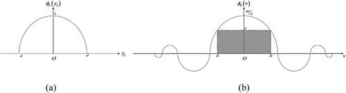
Figure 5. The variation of the basis functions ${\varphi }_n\left(y_1\right)$.

4. Some illustrative examples

In order to see the applicability as well as the accuracy of the above-mentioned method one has considered the illustrative examples where the cross-section $B$ of the cylindrical body $D$ is assumed to be composed by one and several disjoint parts as shown in Figure 6a,b. In these examples for the sake of mathematical calculations simplicity the cross-section $B$ mentioned above has been chosen in different rectangular forms and the cylindrical body is supposed to consist of a simple material which has $\upsilon \left(x^{\mathrm{\prime }}\right)=0.01$. As it is well-known, in the real applications of an inverse problem the data which should be collected by measurements are obtained here synthetically by solving the corresponding direct problem via Born approximation (see Appendix C).

Figure 6. The geometries and the parameters for the illustrative examples. (a) Single cross-sectional case for $B$, (b) Case of several disjoint parts for $B$.

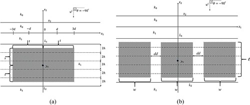
Since the position of the buried body $D$ in a half-space is unknown beforehand then the layered region is supposed to be defined by $y_2\in \left(L_2,L_1\right)$ with $L_2<L_1<0$, because of the necessity for the numerical computations. It is obvious that the method established in this work yields an object function $\upsilon \left(x^{\mathrm{\prime }}\right)$ which is different from zero when the body is located totally or partially in the region $y_2\in \left(L_2,L_1\right)$. Otherwise it gives $\upsilon \left(x^{\mathrm{\prime }}\right)=0$. To observe this particularity, one considers firstly a buried body $D$ that is composed by a single cross-section $B$. In all these different situations of this case which are presented in Figures 7–9 the common parameters for the simple given by Figure 6a are chosen as $\upsilon \left(x^{\mathrm{\prime }}\right)=0.01$, $k_0=2\pi /{\lambda }_0$, $k_1=1.17k_0$, $\theta =-{90}^0$, $x_2=0.25{\lambda }_0$,, $L_1=-0.2{\lambda }_0$, $L_2=-0.3{\lambda }_0$, $t={\lambda }_0$ and $s=0.05{\lambda }_0$. The other parameters related to the method developed here such as number of layers, the half of the thickness of a layer, number of the basis functions, the value appearing in the supports of the basis functions and the Tikhonov regularization parameter are also considered by $M=20$, $h=0.0025{\lambda }_0$, $N=10$, $d=0.33{\lambda }_0$ and $\tau =0.1$, respectively. The wave-lenght ${\lambda }_0$which is seen in the above-mentioned parameters is considered to be equal to 1 m.

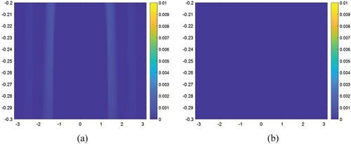
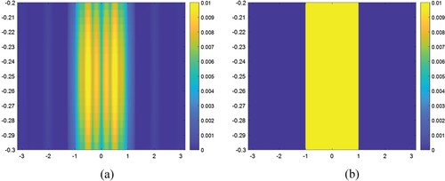
From Figure 7a one can easily conclude that the object function $\upsilon \left(x^{\mathrm{\prime }}\right)$ which is obtained by using the method given in this work is naught as expected. The reason for this result is that $y_0$appearing in Figure 6a is chosen to be $-0.5{\lambda }_0$, thus the body $D$ is completely out of the region $y_2\in \left(L_2,L_1\right)$ as shown in Figure 7b.

Figure 7. The computed and exact values of the object function $\upsilon \left(x^{\mathrm{\prime }}\right)$ for the case where the body$D$is completely out of the region $y_2\in \left(L_2,L_1\right)$. (a) Computed solution, (b) Exact solution.

The computed result given in Figure 8a where $y_0=-0.2{\lambda }_0$ is quite plausible. Because in this case as seen in Figure 8b only the half of the body $D$ exists in the above-mentioned range of $y_2$ and the obtained results show a tendency in this manner.

Figure 8. The computed and exact values of the object function $\upsilon \left(x^{\mathrm{\prime }}\right)$ for the case where a half of the body $D$ is in the region $y_2\in \left(L_2,L_1\right)$. (a) Computed solution, (b) Exact solution.

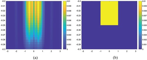
Figure 9. The computed and exact values of the object function $\upsilon \left(x^{\mathrm{\prime }}\right)$ for the case where the body D is completely in the region $y_2\in \left(L_2,L_1\right)$.

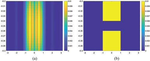
Finally, the result obtained for $y_0=-0.25{\lambda }_0$ where the buried body $D$ is totally assumed to be in the region $y_2\in \left(L_2,L_1\right)$ is presented in Figure 9a. It is obvious that this result is rather good and yields nearly the geometry and as well as the value of the object function considered in the example given by Figure 9b. From Figure 7 and Figure 8 one can easily calculate that the estimated average error between the exact and computed solutions with respect to object function value is nearly 15% and about 0.1% for the geometrical position.

Figure 10. The computed and exact values of the object function $\upsilon \left(x^{\mathrm{\prime }}\right)$ for the case where the cross-section $B$ consists of two disjoint parts. (a) Computed solution, (b) Exact solution.

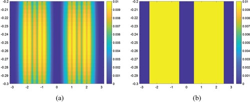
As explained in the introduction one of the main claims of the paper is that the method established here is also available when the cross-section $B$ of the buried $D$ can be composed of several disjoint parts. In order to verify this dissertation, the examples in Figures 10–13b have been considered. In Figure 10b the cross-section $B$ of the body $D$ where its object function $\upsilon \left(x^{\mathrm{\prime }}\right)$ is equal to $0.01$consists of two different parts having the same width and length of $2{\lambda }_0$ and $0.1{\lambda }_0$, respectively. For this case the other parameters such as $k_0$, $k_1$, $\theta$,$M$, $N$, $d$, $h$ and $\tau$are chosen as mentioned above with the distance between two disjoint parts being ${\lambda }_0$.

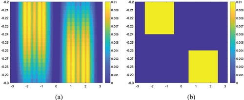
The diagonally overlapping disconnected model is presented in Figure 11b as another example for the case of disjoint parts. Here the centres of the rectangular shapes shown in Figure 11b are given by $\left(-1.5{\lambda }_0,-0.22{\lambda }_0\right)$ and $\left(1.5{\lambda }_0,-0.28{\lambda }_0\right)$ where their width and length are also consider as being $2{\lambda }_0$ and $0.04{\lambda }_0$, respectively. All of the other parameters remain the same with those of previous example.

Figure 11. The computed and exact values of the object function $\upsilon \left(x^{\mathrm{\prime }}\right)$ for the case of diagonally overlapped disjoint parts of $B$. (a) Computed solution, (b) Exact solution.

To observe the situation where the cross-section $B$ of the body $D$ is composed by more than two different separated parts, the example given by in Figure 12b is considered. Here the width and length of the disjoint parts are chosen as being ${\lambda }_0$ and $0.1{\lambda }_0$ respectively. The distance between the successive disjoint parts has the same value ${\lambda }_0$ and the other parameters are also identical with those of previous samples.

Figure 12. The computed and exact values of the object function $\upsilon \left(x^{\mathrm{\prime }}\right)$ for the case where the cross-section $B$ consists of three successive disjoint parts. (a) Computed solution, (b) Exact solution.

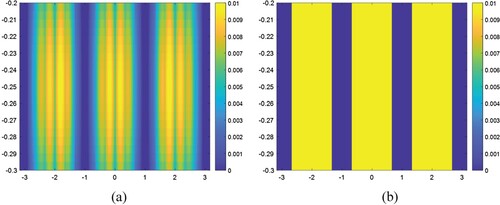
As it can be concluded from the computed solutions presented in Figure 10 and Figure 12a the hybrid method developed in this study processes well into the case where the buried body $D$ has several disjoint cross-sections, too. The results are rather in good resolutions and give satisfying idea about the geometry and as well the value of the object function $\upsilon \left(x^{\mathrm{\prime }}\right)$ of $D$.

Finally, in this stage of disconnected parts, the result obtained for the full overlapped case (see Figure 13b) related to the cross-sections existing in diagonally one is presented in Figure 13a. In this state, it is clear that the method established here cannot distinguish the two disjoint parts of $B$, and it detects them as unified. This result can be interpreted as the most obvious weakness of the presented method. However, this situation is the typical common feature that can be observed in all of the developing techniques which are based to solve inverse scattering problems related to buried bodies.

Figure 13. The computed and exact values of the object function $\upsilon \left(x^{\mathrm{\prime }}\right)$ for the case of full overlapped disjoint parts of $B$. (a) Computed solution, (b) Exact solution.

It is also worthwhile to notice that in all the examples which exhibit the results in Figures 7–13a the Tikhonov regularization is met as its parameter value $\tau =0.1$ satisfies the condition in (38) and the thickness $2h=0.005{\lambda }_0$ of the layer is quite small with respect to ${\lambda }_0$.

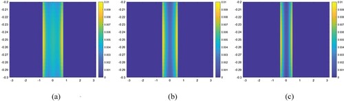
Another important parameter of the proposed method in this paper that its effect needs to be analyzed is the support $2d$ of the basis functions. In all the previous numerical examples $d$ is chosen as being ${\lambda }_0/3$ in accordance with the criterion express by (65). In order to verify the mentioned criterion, the buried body $D$ is considered as in Figure 9b and the results related to some different values of $d$ that have the contradiction to the expression given by (65) are computed and presented in Figure 14a–c. As it can be easily checked from these figures the position and also object function $\upsilon \left(x^{\mathrm{\prime }}\right)$ of the body $D$ become more different than the exact solution with decreasing value of $d$ from ${\lambda }_0/4$ and consequently deteriorate as expected.

Figure 14. The computed results of the object functions related to different values of $d$. (a) $d={\lambda }_0/5$, (b) $d={\lambda }_0/6$, (c) $d={\lambda }_0/7$.

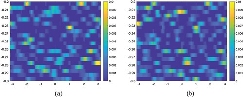
To show the necessity and as well the effect of the regularization technique on the solution of the corresponding ill-posed inverse problem which is obtained by using the hybrid method given in this work, the situation where there is no regularization is observed by choosing the parameter $\tau$ being equal to zero and the corresponding results are presented in Figure 15a,b. In all these examples the buried body $D$ is consider as it is in Figure 9b and Figure 12b, respectively. It can be easily seen from the Figure 15a,b the non-regularized results are extremely poor and do not provide any information about either the location or the constitutive parameters of the buried body.

Figure 15. The computed results for the non-regularized situation. (a) Single cross-sectional case, (b)Triple cross-sectional case.

Finally, in this part of the work to compare the proposed method with some alternative ones which are previously published, numerical examples given in [31,32] and [47] are considered.

In [32,31] where the two-dimensional inverse problem is solved by using an iterative algorithm of the algebraic reconstruction technique (ART), the illustrative examples for the buried bodies are conceived to be as they are in Figure 16b and Figure 17b, respectively (See also Figure 3 of [31,32]). From the comparison of the result in Figure 16a with those of Figures 4–7 in [32] and Figure 17a with Figure 5 in [31] one can easily conclude that these two different methods exhibit almost the same geometries and the object function values for the observed samples. While the common method used in [31,32] requires a certain member of iteration with different incident angles, the fact that the non-iterative hybrid method developed here gives the same result with a single incidence angle can be interpreted as an advantage of the present method over the one in [31,32]. It would also be appropriate to note that the problem considered in [31] and in this study are completely identical except their solution techniques, while the problem in [32], beside its solution method, it is also slightly different from the one discussed in this work with respect to structure where the half-space involving the buried body is terminated by an impedance plane which provides a positive additional contribution to the solution of the problem.

Figure 16. The computed and exact solutions of the object function $\upsilon \left(x^{\mathrm{\prime }}\right)$ considered as an illustrative in [32]. (a) Computed solution, (b) Exact solution

Figure 17. The computed and exact solutions of the object function $\upsilon \left(x^{\mathrm{\prime }}\right)$ considered as an illustrative in [31]. (a) Computed solution, (b) Exact solution.

Since the geometry of sampling buried body in [47] is different than the rectangular geometry that is considered for the sake of simplicity in this paper, the comparison of the results can only be done with respect to the identical value $\upsilon \left(x^{\mathrm{\prime }}\right)=0.01$ of the object functions related to the examples given in both studies. From Figure 9a and Figure 8 presented in this paper and [47], respectively, it is an easy matter to conclude that the results obtain for the buried bodies illuminated by two different types of incident waves which are Gaussian beam in [47] and plane wave in this paper are quite similar and both of these methods are effectives to determine the shape and the values of the object functions.

5. Conclusion and concluding remarks

From the results obtained in the illustrative applications considered in Section 4 one concludes that the proposed hybrid method established in the present work is highly effective in solving two-dimensional inverse scattering problems numerically. The consideration of the convenient choices of the basis functions having the minimum duration in the horizontal direction and the thickness of the layers in the vertical direction, along with the Tikhonov regularization, constitutes a perfect combined solution technique for the full determination of the buried bodies. Consequently, they act together to minimize the effect of the ill-posedness related to inverse scattering problems.

The present work is devoted to the case where all the materials are non-magnetic and the half-spaces are non-conducting i.e.: ${\mu }_0={\mu }_1\equiv \mu \left(x^{\mathrm{\prime }}\right)$ while $k_0$, $k_1$ are real. The contrary cases are also important from practical points of view and merit to be investigated.

Another potential forthcoming study that can be cited here is to determine the similar basis functions which will be used instead of the layers for the variation of the object function with respect to vertical coordinate $y_2$.

Acknowledgement

The authors are indebted to the reviewers for their valuable suggestions and comments which highly improve the quality of the work.

Disclosure statement

No potential conflict of interest was reported by the author(s).

Appendices

Appendix A: The validity of Stokes theorem in the sense of distribution

Here we will show that the classical procedure to yield the Stokes Theorem is also valid in the sense of distribution. For this purpose, $f\left(x\right)$ being a known function, $x\in {\mathbb{R}}^2$and $k$ constant let us consider the Helmholtz equation written by (A1) $\mathrm{\Delta }u\left(x\right)+k^{2}u\left(x\right)=f\left(x\right).$(A1) In order to solve (A1) for $u\left(x\right)$ by a Green’s function method one has to take into account the equation (A2) $\mathrm{\Delta }G\left(x,y\right)+k^{2}G\left(x,y\right)=-\delta \left(x-y\right)$(A2) which is satisfied by two-dimensional Green’s function i.e: $G\left(x,y\right)$. Here $\delta (.)$ is a well-known Dirac distribution and $y\in {\mathbb{R}}^2$. The explicit expression of the two-dimensional Green’s function appearing in (A2) is presented by (A3) $G\left(x,y\right)=-\frac{1}{4i}{H}_0^{\left(1\right)}\left(k|x-y|\right)$(A3) where $H_0^{\left(1\right)}(.)$ is the first kind zeroth order Hankel function. It is also worthwhile to notice that the asymptotic behaviours of this Green’s function and its derivative with respect to its argument for $x\to y$ are given by (A4) $G\left(x,y\right)\sim -\frac{1}{2\pi }\ln \left(\frac{|x-y|}{2}\right)$(A4) and (A5) $\frac{\mathrm{\partial }}{\mathrm{\partial }|x-y|}G\left(x,y\right)\sim -\frac{1}{2\pi |x-y|}.$(A5) Now let us multiply both side of (A1) and (A2) by $G\left(x,y\right)$ and $u\left(x\right)$ respectively, and subtract the obtained terms from each other to write (A6) $G\left(x,y\right)\mathrm{\Delta }u\left(x\right)-u\left(x\right)\mathrm{\Delta }G\left(x,y\right)=G\left(x,y\right)f\left(x\right)+u\left(x\right)\delta \left(x-y\right).$(A6) Since the point $y$ is outside of the region $S_{ϵ}$ shown in Fig. A1 it is obvious that the integration of (A6) on $S_{ϵ}$ gives (A7) ${\int }_{S_{ϵ}}\left[G\left(x,y\right)\mathrm{\Delta }u\left(x\right)-u\left(x\right)\mathrm{\Delta }G\left(x,y\right)\right]dx={\int }_{S_{ϵ}}G\left(x,y\right)f\left(x\right)dx.$(A7) Now let us apply the Stokes’ Theorem on the left side of (A7) which yields (A8) ${\int }_{C+C_{ϵ}+C_1+C_2}\left[G\frac{\mathrm{\partial }u}{\mathrm{\partial }n}-u\frac{\mathrm{\partial }G}{\mathrm{\partial }n}\right]dl={\int }_{S_{ϵ}}G\left(x,y\right)f\left(x\right)dx$(A8) with $C+C_{ϵ}+C_1+C_2$and $n$ being a contour of the region $S_{ϵ}$ and the direction of the unit vector depicted in Figure A1, respectively. It is evident that the functions $G\left(x,y\right)$, $u\left(x\right)$ and their derivatives with respect to $n$ are continuous on $C_1$ and $C_2$. Then (A9) ${\int }_{C_1+C_2}\left[G\frac{\mathrm{\partial }u}{\mathrm{\partial }n}-u\frac{\mathrm{\partial }G}{\mathrm{\partial }n}\right]dl=0$(A9) and (A8) reduces to (A10) ${\int }_C\left[G\frac{\mathrm{\partial }u}{\mathrm{\partial }n}-u\frac{\mathrm{\partial }G}{\mathrm{\partial }n}\right]dl={\int }_{S_{ϵ}}G\left(x,y\right)f\left(x\right)dx-{\int }_{C_{ϵ}}\left[G\frac{\mathrm{\partial }u}{\mathrm{\partial }n}-u\frac{\mathrm{\partial }G}{\mathrm{\partial }n}\right]dl$(A10) By considering the limit of (A10) for $ϵ=|x-y|\to 0$ with (A4) and (A5) as well, one can easily writes that (A11) $\begin{array}{rl}{\int }_C\left[G\frac{\mathrm{\partial }u}{\mathrm{\partial }n}-u\frac{\mathrm{\partial }G}{\mathrm{\partial }n}\right]dl& ={\int }_{S}G\left(x,y\right)f\left(x\right)dx-{\int }_{2\pi }^0\underset{ϵ\to 0}{lim}\left[-\frac{1}{2\pi }\ln \left(\frac{ϵ}{2}\right)\frac{\mathrm{\partial }u}{\mathrm{\partial }n}+\frac{1}{2\pi ϵ}u\right]ϵd\varphi \\ & ={\int }_{S}G\left(x,y\right)f\left(x\right)dx+\frac{1}{2\pi }{\int }_0^{2\pi }\underset{x\to y}{lim}u\left(x\right)d\varphi \\ & =u\left(y\right)+{\int }_{S}G\left(x,y\right)f\left(x\right)dx\end{array}$(A11) where $S=\underset{ϵ\to 0}{lim}{S}_{ϵ}$ is the region surrendered by the contour $C$.

Finally, let us integrate directly both side of (A6) on the above-mentioned region $S$ where $y\in S$. It is an easy matter to show that this one results (A12) ${\int }_S\left[G\left(x,y\right)\mathrm{\Delta }u\left(x\right)-u\left(x\right)\mathrm{\Delta }G\left(x,y\right)\right]dx=u\left(y\right)+{\int }_{S}G\left(x,y\right)f\left(x\right)dx$(A12) The comparison of the latter expression with (A11) yields the relation (A13) ${\int }_S\left[G\left(x,y\right)\mathrm{\Delta }u\left(x\right)-u\left(x\right)\mathrm{\Delta }G\left(x,y\right)\right]dx={\int }_C\left[G\frac{\mathrm{\partial }u}{\mathrm{\partial }n}-u\frac{\mathrm{\partial }G}{\mathrm{\partial }n}\right]dl$(A13) which is nothing but the proof for the validity of classical Stokes’ Theorem in the sense of distribution too. Moreover, we would like to emphasize that the above-mentioned proof which is realized in a homogeneous medium can also be generalized into a multi-part space case. For this purpose, as an example of two-part space which constitutes one of the subjects of this paper, it is sufficient to repeat the operational procedures explained in this section by considering the regions and contours given in Figure A2.

Figure A1. The region $S_{ϵ}$ and its contour lines.

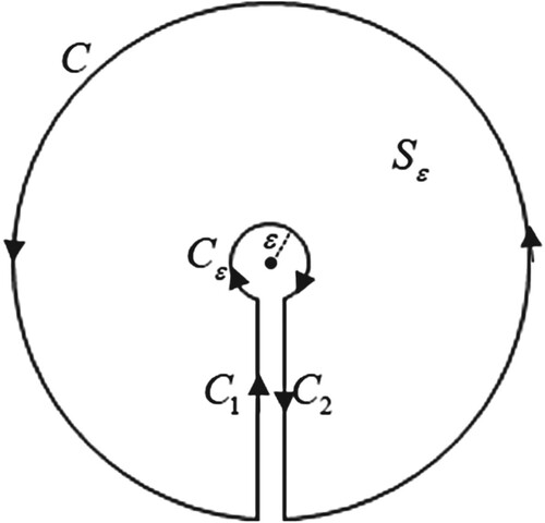
Figure A2. The regions and their contour lines for the two-part space case.

Appendix B: the determination of the Euler equation related to the functional given by (51)

Let us consider an integral given by (B1) $\tilde{I}={\int }_{{\xi }_1}^{{\xi }_2}\tilde{L}\left[\xi ,{\varphi }_0\left(\xi \right),{{\varphi }^{\mathrm{\prime }}}_0\left(\xi \right)\right]d\xi$(B1) where $\tilde{L}\left[\xi ,{\varphi }_0\left(\xi \right),{{\varphi }^{\mathrm{\prime }}}_0\left(\xi \right)\right]$ is a functional operator related to bounded function ${\varphi }_0\left(\xi \right)$ and its derivative ${\varphi }_0^{\mathrm{\prime }}\left(\xi \right)$ such that ${\varphi }_0\left({\xi }_1\right)={\varphi }_0\left({\xi }_2\right)=0$. To obtain the extremum of the integral (B1) for ${\varphi }_0\left(\xi \right)$ which is the problem in question, one has to write first (B2) $\tilde{I}\left(\widetilde{ϵ}\right)={\int }_{{\xi }_1}^{{\xi }_2}\tilde{L}\left[\xi ,{\varphi }_0\left(\xi \right)+\widetilde{ϵ}\tilde{f}\left(\xi \right),{{\varphi }^{\mathrm{\prime }}}_0\left(\xi \right)+\widetilde{ϵ}{\tilde{f}}^{\mathrm{\prime }}\left(\xi \right)\right]d\xi$(B2) with $\widetilde{ϵ}$ and $\tilde{f}\left(\xi \right)$ being a constant and arbitrary function, respectively and then to investigate the solution for the equation (B3) ${\frac{d\tilde{I}\left(\widetilde{ϵ}\right)}{d\widetilde{ϵ}}|}_{\widetilde{ϵ}=0}={\int }_{{\xi }_1}^{{\xi }_2}{\frac{d}{d\widetilde{ϵ}}\tilde{L}\left[\xi ,{\varphi }_0\left(\xi \right)+\widetilde{ϵ}\tilde{f}\left(\xi \right),{{\varphi }^{\mathrm{\prime }}}_0\left(\xi \right)+\widetilde{ϵ}{\tilde{f}}^{\mathrm{\prime }}\left(\xi \right)\right]|}_{\widetilde{ϵ}=0}d\xi =0$(B3) From the well-known chain rule for a derivative, it is an easy matter to show that (B4) $\begin{array}{rl}& {\frac{d}{d\widetilde{ϵ}}\tilde{L}\left[\xi ,{\varphi }_0\left(\xi \right)+\widetilde{ϵ}\tilde{f}\left(\xi \right),{{\varphi }^{\mathrm{\prime }}}_0\left(\xi \right)+\widetilde{ϵ}{\tilde{f}}^{\mathrm{\prime }}\left(\xi \right)\right]|}_{\widetilde{ϵ}=0}\\ & =\frac{d\tilde{L}\left[\xi ,{\varphi }_0\left(\xi \right),{{\varphi }^{\mathrm{\prime }}}_0\left(\xi \right)\right]}{d{\varphi }_0\left(\xi \right)}\tilde{f}\left(\xi \right)+\frac{d\tilde{L}\left[\xi ,{\varphi }_0\left(\xi \right),{{\varphi }^{\mathrm{\prime }}}_0\left(\xi \right)\right]}{d{{\varphi }^{\mathrm{\prime }}}_0\left(\xi \right)}{\tilde{f}}^{\mathrm{\prime }}\left(\xi \right).\end{array}$(B4) By substituting (B4) in (B3) and computing the corresponding integral with the consideration of $\tilde{f}\left({\xi }_1\right)=\tilde{f}\left({\xi }_2\right)=0$ one gets (B5) ${\int }_{{\xi }_1}^{{\xi }_2}\tilde{f}\left(\xi \right)\left[\frac{d\tilde{L}\left[\xi ,{\varphi }_0\left(\xi \right),{{\varphi }^{\mathrm{\prime }}}_0\left(\xi \right)\right]}{d{\varphi }_0\left(\xi \right)}-\frac{d}{d\xi }\frac{d\tilde{L}\left[\xi ,{\varphi }_0\left(\xi \right),{{\varphi }^{\mathrm{\prime }}}_0\left(\xi \right)\right]}{d{{\varphi }^{\mathrm{\prime }}}_0\left(\xi \right)}\right]d\xi =0$(B5) It is obvious that the equality in (B5) can only be satisfied for any arbitrary function $\tilde{f}\left(\xi \right)$ when (B6) $\frac{d\tilde{L}\left[\xi ,{\varphi }_0\left(\xi \right),{{\varphi }^{\mathrm{\prime }}}_0\left(\xi \right)\right]}{d{\varphi }_0\left(\xi \right)}-\frac{d}{d\xi }\frac{d\tilde{L}\left[\xi ,{\varphi }_0\left(\xi \right),{{\varphi }^{\mathrm{\prime }}}_0\left(\xi \right)\right]}{d{{\varphi }^{\mathrm{\prime }}}_0\left(\xi \right)}=0$(B6) The comparison of (51) with (B1) reveals that ${\xi }_2=-{\xi }_1=d$ and $\tilde{L}\left[\xi ,{\varphi }_0\left(\xi \right),{{\varphi }^{\mathrm{\prime }}}_0\left(\xi \right)\right]={\varphi }_0^2-{\eta }^2{\varphi }_0^2$. The consideration of this later expression in (B6) evidently presents the equation given by (52).

Appendix C: the synthetic data collection by using Born approximation

The values of ${\hat{u}}_D\left(v_t,x_2\right)$ appearing in (33), which should be obtained in real application from the measured values of $u\left(x_1,x_2\right)$ on the line $x_2=\text{constant}$, can be found very easily by solving the corresponding direct scattering problem. In this context, since the value of $\upsilon \left(x^{\mathrm{\prime }}\right)$ considered in the illustrative example in Section 4 is sufficiently small, from (16) one writes (C1) $\begin{array}{rl}{u}_D\left(x^{\mathrm{\prime }}\right)& =k_1^2{\int }_B{G}_0\left(x^{\mathrm{\prime }},y^{\mathrm{\prime }}\right)\upsilon \left(y^{\mathrm{\prime }}\right)\left[u_0\left(y^{\mathrm{\prime }}\right)+u_D\left(y^{\mathrm{\prime }}\right)\right]d{y}^{\mathrm{\prime }}\\ & =u_D^{\left(1\right)}\left(x^{\mathrm{\prime }}\right)+k_1^2{\int }_B{G}_0\left(x^{\mathrm{\prime }},y^{\mathrm{\prime }}\right)\upsilon \left(y^{\mathrm{\prime }}\right)u_D\left(y^{\mathrm{\prime }}\right)d{y}^{\mathrm{\prime }}\\ & =u_D^{\left(1\right)}\left(x^{\mathrm{\prime }}\right)+k_1^2{\int }_B{G}_0\left(x^{\mathrm{\prime }},y^{\mathrm{\prime }}\right)\upsilon \left(y^{\mathrm{\prime }}\right)u_D^{\left(1\right)}\left(y^{\mathrm{\prime }}\right)d{y}^{\mathrm{\prime }}+\dots \end{array}$(C1) in serial form with (C2) $u_D^{\left(1\right)}\left(x^{\mathrm{\prime }}\right)=k_1^2{\int }_B{G}_0\left(x^{\mathrm{\prime }},y^{\mathrm{\prime }}\right)\upsilon \left(y^{\mathrm{\prime }}\right)u_0\left(y^{\mathrm{\prime }}\right)d{y}^{\mathrm{\prime }}.$(C2) From this latter, by using the Schwarz inequality [48] it is obvious to get (C3) $|u_D^{\left(1\right)}\left(x^{\mathrm{\prime }}\right)|\le k_1^2\sqrt{{{\int }_B|G_0\left(x^{\mathrm{\prime }},y^{\mathrm{\prime }}\right)u_0\left(y^{\mathrm{\prime }}\right)|}^{2}d{y}^{\mathrm{\prime }}}.\sqrt{{\int }_B{|\upsilon \left(y^{\mathrm{\prime }}\right)|}^{2}d{y}^{\mathrm{\prime }}}$(C3) which yields (C4) $|u_D^{\left(1\right)}\left(x^{\mathrm{\prime }}\right)|=O\left(k_1^2||\upsilon ||\right)$(C4) for small $||\upsilon ||\stackrel{\Delta }{=}\sqrt{{\int }_B{|\upsilon \left(y^{\mathrm{\prime }}\right)|}^{2}d{y}^{\mathrm{\prime }}}$. By considering this relation in the second term appearing on the right-hand side of (C1) one can easily show that (C5) $\begin{array}{cc}\left|k_1^2{\int }_B{G}_0\left(x^{\mathrm{\prime }},y^{\mathrm{\prime }}\right)\upsilon \left(y^{\mathrm{\prime }}\right)u_D^{\left(1\right)}\left(y^{\mathrm{\prime }}\right)d{y}^{\mathrm{\prime }}\right|\le & k_1^2|u_D^{\left(1\right)}\left(x^{\mathrm{\prime }}\right){|}_{max}{\int }_B|G_0\left(x^{\mathrm{\prime }},y^{\mathrm{\prime }}\right)\upsilon \left(y^{\mathrm{\prime }}\right)|d{y}^{\mathrm{\prime }}\\ \le k_1^{2}O\left(k_1^2||\upsilon ||\right)\sqrt{{{\int }_B|G_0\left(x^{\mathrm{\prime }},y^{\mathrm{\prime }}\right)|}^{2}d{y}^{\mathrm{\prime }}}\sqrt{{\int }_B{|\upsilon \left(y^{\mathrm{\prime }}\right)|}^{2}d{y}^{\mathrm{\prime }}}\\ \le O\left(k_1^4{||\upsilon ||}^2\right).\end{array}$(C5) Hence, by neglecting the above-mentioned term of order $k_1^4||\upsilon |{|}^2$ in (C1), which is legitimated in the example considered in this work, one writes (C6) $u_D\left(x^{\mathrm{\prime }}\right)\cong u_D^{\left(1\right)}\left(x^{\mathrm{\prime }}\right).$(C6) This is the well-known Born approximation [49] for the solution of the integral equation (C1). The Born approximated value of the scattered field related to the rectangular cross-sectional cylindrical body which is presented in Fig.6.a can be computed from (C6) with the use of the integral in (C2). For this purpose, also by considering that $\upsilon \left(y^{\mathrm{\prime }}\right)={\upsilon }_0$ is constant in the region $B$ one can first write (C7) $u_D\left(x^{\mathrm{\prime }}\right)\cong k_1^2{\upsilon }_0{\int }_B{G}_0\left(x^{\mathrm{\prime }},y^{\mathrm{\prime }}\right)u_0\left(y^{\mathrm{\prime }}\right)d{y}^{\mathrm{\prime }}=k_1^2{\upsilon }_0{\int }_{-t}^t{\int }_{y_{0-s}}^{y_0+s}{G}_0\left(x_1,x_2;y_1,y_2\right)u_0\left(y_1,y_2\right)d{y}_{2}d{y}_1.$(C7) Subsequently by taking the Fourier transform of this expression with respect to $x_1$ and also substituting (3) and (22) for their corresponding terms which appear in the obtained integral one gets (C8) $\begin{array}{rl}{\hat{u}}_D\left(v,x_2\right)\cong & k_1^2{\upsilon }_0{\int }_{-t}^t{\int }_{y_0-s}^{y_0+s}{\hat{G}}_0\left(v,x_2,y_1,y_2\right)u_0(y_1,y_2)d{y}_{2}d{y}_1\\ & \cong k_1^2{\upsilon }_0{\int }_{-t}^t{\int }_{y_0-s}^{y_0+s}\frac{e^{-iv{y}_1+\text{β}\left(v\right)y_2-\alpha \left(v\right)x_2}}{\alpha \left(v\right)+\text{β}\left(v\right)}T{e}^{i{k}_1\left(y_1\cos \chi +y_2\sin \chi \right)}d{y}_{2}d{y}_1.\end{array}$(C8) It is an easy matter to show that the evaluation of the integral in (C8) yields (C9) ${\hat{u}}_D\left(v,x_2\right)\cong \frac{4T{k}_1^2{\upsilon }_0{e}^{-\alpha \left(v\right)x_2}{e}^{\left[\text{β}\left(v\right)+i{k}_1\sin \chi \right]y_0}\sin \left[\left(k_1\cos \chi -v\right)t\right]\sinh \left[\left(\text{β}\left(v\right)+i{k}_1\sin \chi \right)s\right]}{\left[\alpha \left(v\right)+\text{β}\left(v\right)\right]\left[\text{β}\left(v\right)+i{k}_1\sin \chi \right]\left(k_1\cos \chi -v\right)}$(C9) where $T$, $\chi$, $\alpha \left(v\right)$ and $\text{β}\left(v\right)$ are given by (5), (6) and (23), respectively.

References

- Aïcha IB, Hu GH, Vashisth M, et al. Uniqueness for time-dependent inverse problems with single dynamical data. J Math Anal Appl. 2021;497(2):124910. doi:10.1016/j.jmaa.2020.124910
- Aktosun T, Van Der Mee C. Solution of the inverse scattering problem for the three-dimensional Schrödinger equation using a Fredholm integral equation. SIAM J Math Anal. 1991;22(3):717–731. doi:10.1137/0522043
- Colton DL, Kress R, Kress R. Inverse acoustic and electromagnetic scattering theory. Berlin: Springer; 1998.
- Newton RG. Inverse scattering. II. Three dimensions. J Math Phys. 1980;21(7):1698–1715. doi:10.1063/1.524637
- Liu X, Zhang B. Direct and inverse obstacle scattering problems in a piecewise homogeneous medium. SIAM J Appl Math. 2010;70(8):3105–3120. doi:10.1137/090777578
- Ramm AG. Scattering by an obstacle. Dordrecht: Springer; 1986. p. 14–83
- Idemen M. On different possibilities offered by the Born approximation in inverse scattering problems. Inverse Prob. 1989;5(6):1057. doi:10.1088/0266-5611/5/6/012
- Idemen M, Akduman I. Two-dimensional inverse scattering problems connected with bodies buried in a slab. Inverse Prob. 1990;6(5):749. doi:10.1088/0266-5611/6/5/006
- Abubakar A, Hu W, Van Den Berg PM, et al. A finite-difference contrast source inversion method. Inverse Prob. 2008;24(6):065004. doi:10.1088/0266-5611/24/6/065004
- Bozza G, Estatico C, Pastorino M, et al. An inexact newton method for microwave reconstruction of strong scatterers. IEEE Antennas Wirel Propag Lett. 2006;5:61–64. doi:10.1109/LAWP.2006.870360
- Truong T, Nguyen DL, Klibanov MV. Convexification numerical algorithm for a 2D inverse scattering problem with backscatter data. Inverse Probl Sci Eng. 2021;29(13):2656–2675. doi:10.1080/17415977.2021.1943384
- Cui TJ, Chew WC, Aydiner AA, et al. Inverse scattering of two-dimensional dielectric objects buried in a lossy earth using the distorted Born iterative method. IEEE Trans Geosci Remote Sens. 2001;39(2):339–346. doi:10.1109/36.905242
- Lavarello R, Oelze ML. P4D-4 image reconstruction of moderate contrast targets using the distorted born iterative method. In: Marjorie Passini-Yuhas, editor. 2007 IEEE ultrasonics symposium proceedings. New York: IEEE Ultrasonics, Ferroelectrics, and Frequency Control Society; 2007. p. 1993–1996.
- Liu K, Xu Y, Zou J. A parallel radial bisection algorithm for inverse scattering problems. Inverse Probl Sci Eng. 2013;21(2):197–209. doi:10.1080/17415977.2012.686498
- Li L, Zheng H, Li F. Two-dimensional contrast source inversion method with phaseless data: TM case. IEEE Trans Geosci Remote Sens. 2008;47(6):1719–1736.
- Sun S, Kooij BJ, Yarovoy JT, et al. Cross-correlated contrast source inversion. IEEE Trans Antennas Propag. 2017;65(5):2592–2603. doi:10.1109/TAP.2017.2673758
- Van Den Berg PM, Abubakar A, Fokkema JT. Multiplicative regularization for contrast profile inversion. Radio Sci. 2003;38(2):23–21. doi:10.1029/2001RS002555
- Olson LG, Throne RD. An inverse problem approach to stiffness mapping for early detection of breast cancer. Inverse Probl Sci Eng. 2013;21(2):314–338. doi:10.1080/17415977.2012.700710
- Yu W, Peng Z, Jen L. A fast convergent method in electromagnetic inverse scattering. IEEE Trans Antennas Propag. 1996;44(11):1529–1532. doi:10.1109/8.542078
- Zaiping N, Yerong Z. Hybrid born iterative method in low-frequency inverse scattering problem. IEEE Trans Geosci Remote Sens. 1998;36(3):749–753. doi:10.1109/36.673668
- Zaiping N, Feng Y, Yanwen Z, et al. Variational born iteration method and its applications to hybrid inversion. IEEE Trans Geosci Remote Sens. 2000;38(4):1709–1715. doi:10.1109/36.851969
- Zakaria A, Lovetri J. Application of multiplicative regularization to the finite-element contrast source inversion method. IEEE Trans Antennas Propag. 2011;59(9):3495–3498. doi:10.1109/TAP.2011.2161564
- Cui TJ, Chew WC. Diffraction tomographic algorithm for the detection of three-dimensional objects buried in a lossy half-space. IEEE Trans Antennas Propag. 2002;50(1):42–49. doi:10.1109/8.992560
- Cui TJ, Chew WC, Aydiner AA, et al. Fast-forward solvers for the low-frequency detection of buried dielectric objects. IEEE Trans Geosci Remot Sens. 2003;41(9):2026–2036. doi:10.1109/TGRS.2003.813502
- Monte LL, Erricolo D, Soldovieri F, et al. Radio frequency tomography for tunnel detection. IEEE Trans Geosci Remote Sens. 2009;48(3):1128–1137. doi:10.1109/TGRS.2009.2029341
- Monte LL, Erricolo D, Soldovieri F, et al. RF tomography for below-ground imaging of extended areas and close-in sensing. IEEE Geosci Remote Sens Lett. 2010;7(3):496–500. doi:10.1109/LGRS.2009.2039918
- Monte LL, Soldovieri F, Erricolo D, et al. Imaging below irregular terrain using RF tomography. IEEE Trans Geosci Remote Sens. 2012;50(9):3364–3373. doi:10.1109/TGRS.2012.2183136
- Gilmore C, et al. A wideband microwave tomography system with a novel frequency selection procedure. IEEE Trans Biomed Eng. 2010;57(4):894–904. doi:10.1109/TBME.2009.2036372
- Gaikovich KP, Maksimovitch YS, Sumin MI. Inverse scattering problems of near-field subsurface pulse diagnostics. Inverse Probl Sci Eng. 2018;26(11):1590–1611. doi:10.1080/17415977.2017.1417405
- Akduman I, Topsakal E. Determination of the orientation of cylindrical bodies buried in a half-space by the use of scattering data. Inverse Prob. 1993;9(2):193. doi:10.1088/0266-5611/9/2/002
- Akduman I, Alkumru A. A generalized ART algorithm for inverse scattering problems related to buried cylindrical bodies. Inverse Prob. 1995;11(6):1125. doi:10.1088/0266-5611/11/6/001
- Alkumru A, Akduman I. Imaging of cylindrical bodies buried in a layered half-space bounded by an impedance plane. AEU Archiv für Elektronik und Übertragungstechnik. 1998;52(1):9–16.
- Chiu CC, Lin CJ. Image reconstruction of buried uniaxial dielectric cylinders. Electromagnetics. 2002;22(2):97–112. doi:10.1080/027263402753455447
- Grisel Y, Fourbil J, Mouysset V. An optimization approach for the localization of defects in an inhomogeneous medium from acoustic far-field measurements at a fixed frequency. Inverse Probl Sci Eng. 2016;24(7):1162–1185. doi:10.1080/17415977.2015.1124426
- Idemen M, Akduman I. On inverse scattering problems related to cylindrical bodies with unknown orientations. Wave Motion. 1993;17(1):33–48. doi:10.1016/0165-2125(93)90087-V
- Idemen M. Inverse scattering problems connected with cylindrical bodies, In: Hashimoto M., Editor. Analytical and numerical methods in electromagnetic wave theory. Tokyo, Japan: Science House Co. Ltd.; 1993. p. 57–122.
- Idemen M. Universal boundary conditions and Cauchy data for the electromagnetic field. In: Akhlesh Lakhtakia, editor. Essays on the formal aspects of electromagnetic theory. Singapore: World Scientific; 1993. p. 657–698.
- Persico R, Bernini R, Soldovieri F. The role of the measurement configuration in inverse scattering from buried objects under the Born approximation. IEEE Trans Antennas Propag. 2005;53(6):1875–1887. doi:10.1109/TAP.2005.848468
- Tsihrintzis GA, Devaney AJ. Higher order (nonlinear) diffraction tomography: inversion of the rytov series. IEEE Trans Inf Theory. 2000;46(5):1748–1761. doi:10.1109/18.857788
- Tabatabaeenejad A, Moghaddam M. Inversion of subsurface properties of layered dielectric structures with random slightly rough interfaces using the method of simulated annealing. IEEE Trans Geosci Remote Sens. 2009;47(7):2035–2046. doi:10.1109/TGRS.2008.2011982
- Winters DW, Van Veen BD, Hagness SC. A sparsity regularization approach to the electromagnetic inverse scattering problem. IEEE Trans Antennas Propag. 2009;58(1):145–154. doi:10.1109/TAP.2009.2035997
- Kress R. Linear integral equations. Berlin: Springer Verlag; 1980.
- Marple SL. Digital Spectral Analysis with Applications, Prentice-Hall, NJ, USA, 1986.
- Kay SM. Modern spectral estimation. New Jersey: Prentice-Hall; 1988.
- Papoulis A. Signal analysis. New York: Mcgraw-Hill College; 1977.
- Gelfand IM, Fomin SV. Calculus of variations prentice-Hall. New Jersey: Englewood Cliffs: Inc; 1963.
- Akduman I. An inverse scattering problem related to buried cylindrical bodies illuminated by Gaussian beams. Inverse Prob. 1994;10:213–226. doi:10.1088/0266-5611/10/2/003
- Oden JT, Demkowicz LF. Applied functional analysis. Chapman and Hall/CRC; 2017.
- Li J, Wang X, Wang T. On the validity of born approximation. Prog Electromagn Res. 2010;107:219–237. doi:10.2528/PIER10070504