Mathematical insights into interval solutions of fuzzy relation inequalities for effective Information resource sharing in business education

Abstract

To examine the connectivity of educational and business institution networks and assess their resource accessibility, we have employed min-max fuzzy relation systems. This piece aims to delve into the outcomes resulting from various factors within a three-compartmental financial system. The research undergoes the dynamical max-min fuzzy solutions, which are expressed in an interval format. These solutions take into consideration variables such as the price index, interest rate, investment demand, fluctuations, cost per investment derived from saved funds, and the elasticity of market demand within the commercial sector. These variables are essential for comprehending the dynamics of the three-compartment financial system. It is difficult to obtain the entire set of solutions for the max-min fuzzy relation system using only minimal solutions. Some of these systems can be solved using optimized fuzzy relation models for both maximal and minimal solutions. Therefore, by converting the business market's financial system into a max-min fuzzy relation inequality, the strategy presented in this article tries to get the broadest and changing solution fluctuating between minimal and maximal solutions. With this suggested strategy for solving the problem, the limiting upper and lower values within which the given quantities fluctuate are identified. By measuring the breadth of the resulting interval, the range of fluctuation may be identified, giving a thorough insight into the system's behaviour. Due to the potential instability of market agents and their respective influences, fluctuations may occur in the demand, supply, and prices of indices in the financial system. Consequently, presenting the financial system in the format of the widest fuzzy interval solution can provide easily accessible information to the general public by illustrating the max-min fuzzy relation system of financial dynamics, outlining the necessary steps, and including a numerical example.

KEYWORDS:

• Fuzzy logic
• three-compartmental financial model
• max-min fuzzy relation inequality system
• peer-to-peer (P2P) network
• fluctuated and widest interval solution

MSC 2020:

• 03E72
• 91-10
• 03B52

1. Introduction

In the field of Algebra, the composition operator typically involves the binary operations of addition and multiplication. This operator is crucial for investigating qualitative relations. However, in certain domains, this analysis has proven to be unstable and has presented certain drawbacks. As a result, the fuzzy addition-multiplication composition has been introduced as a more suitable alternative for binary relations. Several renowned mathematicians have shown interest in this concept and contributed to the development of max-min fuzzy algebra [1–5]. This technique and scheme have found significant applications in the field of computer engineering, particularly in areas such as management and control [6–10].

The composition operator, initially applied to the system of linear equations by Sanchez [11, 12], was named the max-min fuzzy relation system of equations. The algorithm for solving the fuzzy max-min composition equation system significantly differs from the classical system of equations. It has been observed that the total solution set for a consistent max-min fuzzy system is often non-convex, and the condition for obtaining the minimal solution is not unique. The complete solution is obtained by combining the unique maximum solution with a finite number of minimal solutions.

E. Sanchez was the first to apply the fuzzy max-min relation equation in the field of medical diagnosis [12]. The fuzzy max-min composition systems of equality and inequality have been successfully employed to investigate various practical fields. These include fuzzy inference systems [13], imaging compression and reconstruction [14, 15], engineering education [16], media monitoring systems with HTTP guards [17], Peer-to-Peer (P2P) networking systems [18], BitTorrent-like peer-to-peer (BTP2P) script-sharing systems, [19–25], goods supply [26–28], and wire-less system [29, 30]. As far as the contribution and novelty are concerned of this article, we present a stepwise scheme for max-min fuzzy solution of each compartment of financial system in the format of the widest interval solution. This shows the up and down in each quantity from minimum to maximum value in the fuzzy form. This can be comparable with other work when we assign a membership function to that work having some certain limit. Zero is minimum value in fuzzy formate and one is max value, like a probabilistic problem. The solution will be oscillating between these two values.

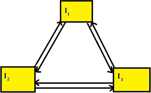
In recent times, the addition-multiplication fuzzy composition system has been applied to file sharing systems for educational purposes [31, 32]. Researchers have contributed and published different types of mathematical model by applying different techniques such as [33–36]. Different finance and fractional models are analysed by the scholars which are available in the literature as [37, 38]. In this context, let us consider applying this composition relation to a business system consisting of three components and their transformations relative to each other, as depicted in Figure 1. In this business market, there are knowledge resources related to the interest rate ${\mathbb{I}}_1$, demand for investing ${\mathbb{I}}_2$, and index of price ${\mathbb{I}}_3$. These quantities undergo transformations that are influenced by parameters and are transferred between the different quantities. The relationship between the agents ${\mathbb{I}}_1$, ${\mathbb{I}}_2$, and ${\mathbb{I}}_3$ is denoted by the width $r_{ij}$. This signifies that when the resources of the j-th quantity are transferred to the i-th quantity, the level of transformation is represented as $r_{ij}\wedge {\mathbb{I}}_i,$Here, ${\mathbb{I}}_i$ represents the quality of transformation level for the three agents in the business market system. Please refer to [39] for a detailed description of the symbols and parameters used in this context. (1) $\begin{array}{rl}\dot{{\mathbb{I}}_1}\left(t\right)& =\eta {\mathbb{I}}_3+{\mathbb{I}}_2{\mathbb{I}}_1-\mathrm{\Omega }{\mathbb{I}}_1\\ \dot{{\mathbb{I}}_2}\left(t\right)& =-K{\mathbb{I}}_2-\left(\alpha \right){\mathbb{I}}_1^2+\lambda \\ \dot{{\mathbb{I}}_3}\left(t\right)& =-\rho {\mathbb{I}}_2-\delta {\mathbb{I}}_1-ϵ{\mathbb{I}}_3,\end{array}$(1) Here K is the expenditure per investment, Ω is for the saving amount, ϵ is the elasticity of local markets demand in commercial field, parameters η, α, λ, ρ, δ are the fixed constants. Let us assume that the quality of transformation level of all three agents is bounded by the values $b_i$ and $d_i$, where (2) $\begin{array}{rl}{b}_1& \le \dot{{\mathbb{I}}_1}\left(t\right)\le d_1\\ b_2& \le \dot{{\mathbb{I}}_2}\left(t\right)\le d_2\\ b_3& \le \dot{{\mathbb{I}}_3}\left(t\right)\le d_3,\end{array}$(2) or (3) $\begin{array}{rl}{b}_1& \le \eta {\mathbb{I}}_3+{\mathbb{I}}_2{\mathbb{I}}_1-\mathrm{\Omega }{\mathbb{I}}_1\le d_1\\ b_2& \le -K{\mathbb{I}}_2-\left(\alpha \right){\mathbb{I}}_1^2+\lambda \le d_2\\ b_3& \le -\rho {\mathbb{I}}_2-\delta {\mathbb{I}}_1-ϵ{\mathbb{I}}_3\le d_3.\end{array}$(3) By conversion of max-min fuzzy composition inequality as follows (4) $\begin{array}{rl}{b}_1& \le (r_{11}\wedge {\mathbb{I}}_1)\vee (r_{12}\wedge {\mathbb{I}}_2)\vee (r_{13}\wedge {\mathbb{I}}_3)\le d_1\\ b_2& \le (r_{21}\wedge {\mathbb{I}}_1)\vee (r_{22}\wedge {\mathbb{I}}_2)\vee (r_{23}\wedge {\mathbb{I}}_3)\le d_2\\ b_3& \le (r_{31}\wedge {\mathbb{I}}_1)\vee (r_{31}\wedge {\mathbb{I}}_2)\vee (r_{33}\wedge {\mathbb{I}}_3)\le d_3,\end{array}$(4) In the article by the scholars [31], they discussed the numerical solutions of the addition-multiplication fuzzy composition system, particularly focusing on the case of an inconsistent system. In related literature, various approaches have been employed to characterize the numerical solutions. For instance, some scholars have utilized the total deviations, which involve calculating the sum of all deviations with respect to each equation of the system. Alternatively, other scholars have focused on the maximum deviation instead of considering the entire set of deviations [31].

Figure 1. Business information resource system of the three compartments.

2. Preliminaries

The system (4(4) $\begin{array}{rl}{b}_1& \le (r_{11}\wedge {\mathbb{I}}_1)\vee (r_{12}\wedge {\mathbb{I}}_2)\vee (r_{13}\wedge {\mathbb{I}}_3)\le d_1\\ b_2& \le (r_{21}\wedge {\mathbb{I}}_1)\vee (r_{22}\wedge {\mathbb{I}}_2)\vee (r_{23}\wedge {\mathbb{I}}_3)\le d_2\\ b_3& \le (r_{31}\wedge {\mathbb{I}}_1)\vee (r_{31}\wedge {\mathbb{I}}_2)\vee (r_{33}\wedge {\mathbb{I}}_3)\le d_3,\end{array}$(4) ) can be written in the short form as (5) $b_i^t\le (B\circ {\mathbb{I}}_i^t)\le d_i^t,$(5) where $B=(r_{ij}{)}_{3\times 3}$, ${\mathbb{I}}_i=({\mathbb{I}}_1,{\mathbb{I}}_2,{\mathbb{I}}_3)$, $b_i=b_1,b_2,b_3$, $d_i=d_1,d_2,d_3$ and “$\circ$” shows the max-min fuzzy composition. Further $\wedge$ is used for conjunction (product) to provide the minimum value, while $\vee$ is for disjunction (addition) to provide the maximum value.

Definition 2.1

[31]

The solution set of the problem (4(4) $\begin{array}{rl}{b}_1& \le (r_{11}\wedge {\mathbb{I}}_1)\vee (r_{12}\wedge {\mathbb{I}}_2)\vee (r_{13}\wedge {\mathbb{I}}_3)\le d_1\\ b_2& \le (r_{21}\wedge {\mathbb{I}}_1)\vee (r_{22}\wedge {\mathbb{I}}_2)\vee (r_{23}\wedge {\mathbb{I}}_3)\le d_2\\ b_3& \le (r_{31}\wedge {\mathbb{I}}_1)\vee (r_{31}\wedge {\mathbb{I}}_2)\vee (r_{33}\wedge {\mathbb{I}}_3)\le d_3,\end{array}$(4) ) is written by $\mathbb{I}(B,b,d)$ i.e $\mathbb{I}(B,b,d)=\{{\mathbb{I}}_i\in [0,1{]}^3|b_i^t\le B\circ {\mathbb{I}}_i^t\le d_i^t\}.$Further, the system (4(4) $\begin{array}{rl}{b}_1& \le (r_{11}\wedge {\mathbb{I}}_1)\vee (r_{12}\wedge {\mathbb{I}}_2)\vee (r_{13}\wedge {\mathbb{I}}_3)\le d_1\\ b_2& \le (r_{21}\wedge {\mathbb{I}}_1)\vee (r_{22}\wedge {\mathbb{I}}_2)\vee (r_{23}\wedge {\mathbb{I}}_3)\le d_2\\ b_3& \le (r_{31}\wedge {\mathbb{I}}_1)\vee (r_{31}\wedge {\mathbb{I}}_2)\vee (r_{33}\wedge {\mathbb{I}}_3)\le d_3,\end{array}$(4) ) will be consistent if $\mathbb{I}(B,b,d)\ne 0,$ other it is inconsistent.

Definition 2.2

[31]

For the problem (4(4) $\begin{array}{rl}{b}_1& \le (r_{11}\wedge {\mathbb{I}}_1)\vee (r_{12}\wedge {\mathbb{I}}_2)\vee (r_{13}\wedge {\mathbb{I}}_3)\le d_1\\ b_2& \le (r_{21}\wedge {\mathbb{I}}_1)\vee (r_{22}\wedge {\mathbb{I}}_2)\vee (r_{23}\wedge {\mathbb{I}}_3)\le d_2\\ b_3& \le (r_{31}\wedge {\mathbb{I}}_1)\vee (r_{31}\wedge {\mathbb{I}}_2)\vee (r_{33}\wedge {\mathbb{I}}_3)\le d_3,\end{array}$(4) ) the solution $\hat{\mathbb{I}}\in \mathbb{I}(B,b,d)$ is called the maximum solution if $\mathbb{I}\le \hat{\mathbb{I}}$ for all $\mathbb{I}\in \mathbb{I}(B,b,d)$. The solution $\check{\mathbb{I}}\in \mathbb{I}(B,b,d)$ is called the minimal solution if $\mathbb{I}\le \check{\mathbb{I}}$ implies that $\mathbb{I}=\check{\mathbb{I}}$

Next for the consistency of system (4(4) $\begin{array}{rl}{b}_1& \le (r_{11}\wedge {\mathbb{I}}_1)\vee (r_{12}\wedge {\mathbb{I}}_2)\vee (r_{13}\wedge {\mathbb{I}}_3)\le d_1\\ b_2& \le (r_{21}\wedge {\mathbb{I}}_1)\vee (r_{22}\wedge {\mathbb{I}}_2)\vee (r_{23}\wedge {\mathbb{I}}_3)\le d_2\\ b_3& \le (r_{31}\wedge {\mathbb{I}}_1)\vee (r_{31}\wedge {\mathbb{I}}_2)\vee (r_{33}\wedge {\mathbb{I}}_3)\le d_3,\end{array}$(4) ), we take a vector $\check{\mathbb{I}}$ for $j\in J$ as (6) ${\mathbb{I}}_j=\{i\in \mathbb{I}|r_{ij}>d_i\}$(6) and we choose the vector $\hat{\mathbb{I}}=({\hat{\mathbb{I}}}_1,{\hat{\mathbb{I}}}_2,{\hat{\mathbb{I}}}_3)$ where (7) $\begin{array}{r}\hat{\mathbb{I}}=\{\begin{array}{ll}1,& {\mathbb{I}}_j=0\\ \underset{i\in {\mathbf{I}}_j}{\bigwedge }{d}_i,& {\mathbb{I}}_j\ne 0.\end{array}\end{array}$(7)

Theorem 2.3

[5–7]

The problem (3(3) $\begin{array}{rl}{b}_1& \le \eta {\mathbb{I}}_3+{\mathbb{I}}_2{\mathbb{I}}_1-\mathrm{\Omega }{\mathbb{I}}_1\le d_1\\ b_2& \le -K{\mathbb{I}}_2-\left(\alpha \right){\mathbb{I}}_1^2+\lambda \le d_2\\ b_3& \le -\rho {\mathbb{I}}_2-\delta {\mathbb{I}}_1-ϵ{\mathbb{I}}_3\le d_3.\end{array}$(3) ) is said to be consistent if the vector $\hat{\mathbb{I}}$ is the solution of problem (3(3) $\begin{array}{rl}{b}_1& \le \eta {\mathbb{I}}_3+{\mathbb{I}}_2{\mathbb{I}}_1-\mathrm{\Omega }{\mathbb{I}}_1\le d_1\\ b_2& \le -K{\mathbb{I}}_2-\left(\alpha \right){\mathbb{I}}_1^2+\lambda \le d_2\\ b_3& \le -\rho {\mathbb{I}}_2-\delta {\mathbb{I}}_1-ϵ{\mathbb{I}}_3\le d_3.\end{array}$(3) ). Furthermore, if the problem (3(3) $\begin{array}{rl}{b}_1& \le \eta {\mathbb{I}}_3+{\mathbb{I}}_2{\mathbb{I}}_1-\mathrm{\Omega }{\mathbb{I}}_1\le d_1\\ b_2& \le -K{\mathbb{I}}_2-\left(\alpha \right){\mathbb{I}}_1^2+\lambda \le d_2\\ b_3& \le -\rho {\mathbb{I}}_2-\delta {\mathbb{I}}_1-ϵ{\mathbb{I}}_3\le d_3.\end{array}$(3) ) is consistent the $\hat{\mathbb{I}}$ is unique maximal solution of the given system.

Really, if system (3(3) $\begin{array}{rl}{b}_1& \le \eta {\mathbb{I}}_3+{\mathbb{I}}_2{\mathbb{I}}_1-\mathrm{\Omega }{\mathbb{I}}_1\le d_1\\ b_2& \le -K{\mathbb{I}}_2-\left(\alpha \right){\mathbb{I}}_1^2+\lambda \le d_2\\ b_3& \le -\rho {\mathbb{I}}_2-\delta {\mathbb{I}}_1-ϵ{\mathbb{I}}_3\le d_3.\end{array}$(3) ) is consistent, it must have a unique maximal solution and minimum solution of finite order. The complete set of solution for problem (3(3) $\begin{array}{rl}{b}_1& \le \eta {\mathbb{I}}_3+{\mathbb{I}}_2{\mathbb{I}}_1-\mathrm{\Omega }{\mathbb{I}}_1\le d_1\\ b_2& \le -K{\mathbb{I}}_2-\left(\alpha \right){\mathbb{I}}_1^2+\lambda \le d_2\\ b_3& \le -\rho {\mathbb{I}}_2-\delta {\mathbb{I}}_1-ϵ{\mathbb{I}}_3\le d_3.\end{array}$(3) ) may be given in the Theorem 2.4.

Theorem 2.4

[40, 41]

When the System (3(3) $\begin{array}{rl}{b}_1& \le \eta {\mathbb{I}}_3+{\mathbb{I}}_2{\mathbb{I}}_1-\mathrm{\Omega }{\mathbb{I}}_1\le d_1\\ b_2& \le -K{\mathbb{I}}_2-\left(\alpha \right){\mathbb{I}}_1^2+\lambda \le d_2\\ b_3& \le -\rho {\mathbb{I}}_2-\delta {\mathbb{I}}_1-ϵ{\mathbb{I}}_3\le d_3.\end{array}$(3) ) is consistent, then the set of solution can be written as $\mathbb{I}(B,b,d)=\underset{\check{\mathbb{I}}\in \check{\mathbb{I}}(B,b,d)}{⨆}[\check{\mathbb{I}},\hat{\mathbb{I}}]$where $\hat{\mathbb{I}}$ is the maximal unique solution and $\hat{\mathbb{I}}(B,b,d)$ is the solution set of all minimal solutions [1–4].

3. Fluctuated interval solution

In this section, we present the definition of the widest and fluctuated interval solution. As mentioned previously, achieving complete (minimal) solutions is not always an easy task, and it may not be necessary in all cases. Some scholars have shown interest in optimizing problems under the fuzzy composition relation [5, 17, 40–43]. However, it has been observed that such solutions can become unstable when subjected to small perturbations. To address this limitation, the concept of the widest interval solution for business system dynamics has been introduced, as outlined in the forthcoming definitions.

Definition 3.1

[31]

Consider $[\acute{\mathbb{I}},\acute{\stackrel{´}{\mathbb{I}}}]\subseteq [0,1]$ such that $\acute{\stackrel{´}{\mathbb{I}}}\le \acute{\mathbb{I}}$ then $\underset{j\in J}{min}\{{\acute{\stackrel{´}{\mathbb{I}}}}_j-{\acute{\mathbb{I}}}_j\}$ is called the width of the given interval which is represented by $w[\acute{\mathbb{I}},\acute{\stackrel{´}{\mathbb{I}}}]$

Definition 3.2

[31]

Let $[\acute{\mathbb{I}},\acute{\stackrel{´}{\mathbb{I}}}]\subseteq [0,1]$ such that $\acute{\stackrel{´}{\mathbb{I}}}\le \acute{\mathbb{I}}$ then $[\acute{\mathbb{I}},\acute{\stackrel{´}{\mathbb{I}}}]$ is called the interval solution of system (3(3) $\begin{array}{rl}{b}_1& \le \eta {\mathbb{I}}_3+{\mathbb{I}}_2{\mathbb{I}}_1-\mathrm{\Omega }{\mathbb{I}}_1\le d_1\\ b_2& \le -K{\mathbb{I}}_2-\left(\alpha \right){\mathbb{I}}_1^2+\lambda \le d_2\\ b_3& \le -\rho {\mathbb{I}}_2-\delta {\mathbb{I}}_1-ϵ{\mathbb{I}}_3\le d_3.\end{array}$(3) ) if $[\acute{\mathbb{I}},\acute{\stackrel{´}{\mathbb{I}}}]\subseteq \mathbb{I}(B,b,d).$

Definition 3.3

[31]

Let $[{\mathbb{I}}^{\ast },{\mathbb{I}}^{\ast \ast }]\subseteq \mathbb{I}(B,b,d)$ be the solution in interval format of system (3(3) $\begin{array}{rl}{b}_1& \le \eta {\mathbb{I}}_3+{\mathbb{I}}_2{\mathbb{I}}_1-\mathrm{\Omega }{\mathbb{I}}_1\le d_1\\ b_2& \le -K{\mathbb{I}}_2-\left(\alpha \right){\mathbb{I}}_1^2+\lambda \le d_2\\ b_3& \le -\rho {\mathbb{I}}_2-\delta {\mathbb{I}}_1-ϵ{\mathbb{I}}_3\le d_3.\end{array}$(3) ), then $[{\mathbb{I}}^{\ast },{\mathbb{I}}^{\ast \ast }]$ is called the widest solution in interval format if $w[{\mathbb{I}}^{\ast },{\mathbb{I}}^{\ast \ast }]\ge w[\acute{\mathbb{I}},\acute{\stackrel{´}{\mathbb{I}}}].$

Theorem 3.4

Let $[\acute{\mathbb{I}},\acute{\stackrel{´}{\mathbb{I}}}],[\acute{\mathbb{J}},\acute{\stackrel{´}{\mathbb{J}}}]\subseteq \mathbb{I}(B,b,d)$ are two solutions in interval formate for the system (3(3) $\begin{array}{rl}{b}_1& \le \eta {\mathbb{I}}_3+{\mathbb{I}}_2{\mathbb{I}}_1-\mathrm{\Omega }{\mathbb{I}}_1\le d_1\\ b_2& \le -K{\mathbb{I}}_2-\left(\alpha \right){\mathbb{I}}_1^2+\lambda \le d_2\\ b_3& \le -\rho {\mathbb{I}}_2-\delta {\mathbb{I}}_1-ϵ{\mathbb{I}}_3\le d_3.\end{array}$(3) ). If $[\acute{\mathbb{I}},\acute{\stackrel{´}{\mathbb{I}}}]\le [\acute{\mathbb{J}},\acute{\stackrel{´}{\mathbb{J}}}]$i.e $\acute{\mathbb{I}}\ge \acute{\mathbb{J}}$ and $\acute{\stackrel{´}{\mathbb{I}}}\le \acute{\stackrel{´}{\mathbb{J}}}$ then $w[\acute{\mathbb{I}},\acute{\stackrel{´}{\mathbb{I}}}]\le w[\acute{\mathbb{J}},\acute{\stackrel{´}{\mathbb{J}}}].$

Proof.

The proof followed from Definition 3.1.

Theorem 3.5

Let system (3(3) $\begin{array}{rl}{b}_1& \le \eta {\mathbb{I}}_3+{\mathbb{I}}_2{\mathbb{I}}_1-\mathrm{\Omega }{\mathbb{I}}_1\le d_1\\ b_2& \le -K{\mathbb{I}}_2-\left(\alpha \right){\mathbb{I}}_1^2+\lambda \le d_2\\ b_3& \le -\rho {\mathbb{I}}_2-\delta {\mathbb{I}}_1-ϵ{\mathbb{I}}_3\le d_3.\end{array}$(3) ) be consistent with maximal solution $\left[\hat{\mathbb{I}}\right]$, then there lie the minimal solution $\left[{\check{\mathbb{I}}}^{\ast }\right]\in \mathbb{I}(B,b,d)$ such that the most fluctuated or wide solution of system (3(3) $\begin{array}{rl}{b}_1& \le \eta {\mathbb{I}}_3+{\mathbb{I}}_2{\mathbb{I}}_1-\mathrm{\Omega }{\mathbb{I}}_1\le d_1\\ b_2& \le -K{\mathbb{I}}_2-\left(\alpha \right){\mathbb{I}}_1^2+\lambda \le d_2\\ b_3& \le -\rho {\mathbb{I}}_2-\delta {\mathbb{I}}_1-ϵ{\mathbb{I}}_3\le d_3.\end{array}$(3) ) is $[{\check{\mathbb{I}}}^{\ast },\hat{\mathbb{I}}].$

Proof.

Consider $[\acute{\mathbb{I}},\acute{\stackrel{´}{\mathbb{I}}}]\subseteq \mathbb{I}(B,b,d)$ be any solution of the proposed system having condition of $\acute{\mathbb{I}}\le \acute{\stackrel{´}{\mathbb{I}}}.$ Now it is quite clear that $\acute{\mathbb{I}},\acute{\stackrel{´}{\mathbb{I}}}\in \mathbb{I}(B,b,d)$. Now by definition of maximal solution (8) $\acute{\stackrel{´}{\mathbb{I}}}\le \hat{\mathbb{I}}.$(8) Next by Theorem 2.4, we can write $\mathbb{I}(B,b,d)=\underset{\check{\mathbb{I}}\in \check{\mathbb{I}}(B,b,d)}{⨆}[\check{\mathbb{I}},\hat{\mathbb{I}}],$here $\check{\mathbb{I}}(B,b,d)$ is the set of minimal solution. As $\acute{\mathbb{I}}\in \mathbb{I}(B,b,d),$ then there lie a minimum solution $\acute{\stackrel{ˇ}{\mathbb{I}}}\in \check{\mathbb{I}}(B,b,d)$ as $\acute{\stackrel{ˇ}{\mathbb{I}}}\in [\acute{\stackrel{ˇ}{\mathbb{I}}},\hat{\mathbb{I}}]$ and this implies that (9) $\acute{\stackrel{ˇ}{\mathbb{I}}}\le \acute{\mathbb{I}}.$(9) Now by (8(8) $\acute{\stackrel{´}{\mathbb{I}}}\le \hat{\mathbb{I}}.$(8) ) and (9(9) $\acute{\stackrel{ˇ}{\mathbb{I}}}\le \acute{\mathbb{I}}.$(9) ) shows that $[\acute{\mathbb{I}},\acute{\stackrel{´}{\mathbb{I}}}]\subseteq [\acute{\stackrel{ˇ}{\mathbb{I}}},\acute{\mathbb{I}}]$ hence this follows from the definition of widest interval solution as (10) $w[\acute{\mathbb{I}},\acute{\stackrel{´}{\mathbb{I}}}]\subseteq w[\acute{\stackrel{ˇ}{\mathbb{I}}},\acute{\mathbb{I}}].$(10) Further it should be noted that $\check{\mathbb{I}}(B,b,d)$ is finite, Therefore, we can write ${\check{\mathbb{I}}}^{\ast }\in \check{\mathbb{I}}(B,b,d)$ having the condition as (11) $w[{\acute{\mathbb{I}}}^{\ast },\hat{\mathbb{I}}]=\underset{\check{\mathbb{I}}\in \check{\mathbb{I}}(B,b,d)}{max}w[\check{\mathbb{I}},\hat{\mathbb{I}}].$(11) As $\acute{\stackrel{ˇ}{\mathbb{I}}}\in \acute{\stackrel{ˇ}{\mathbb{I}}}(B,b,d),$ so we have (12) $\left[\underset{\check{\mathbb{I}}\in \check{\mathbb{I}}(B,b,d)}{max}w\right[\check{\mathbb{I}},\hat{\mathbb{I}}]\ge w[\acute{\stackrel{ˇ}{\mathbb{I}}},\hat{\mathbb{I}}].$(12) Hence (10(10) $w[\acute{\mathbb{I}},\acute{\stackrel{´}{\mathbb{I}}}]\subseteq w[\acute{\stackrel{ˇ}{\mathbb{I}}},\acute{\mathbb{I}}].$(10) ), (11(11) $w[{\acute{\mathbb{I}}}^{\ast },\hat{\mathbb{I}}]=\underset{\check{\mathbb{I}}\in \check{\mathbb{I}}(B,b,d)}{max}w[\check{\mathbb{I}},\hat{\mathbb{I}}].$(11) ), (12(12) $\left[\underset{\check{\mathbb{I}}\in \check{\mathbb{I}}(B,b,d)}{max}w\right[\check{\mathbb{I}},\hat{\mathbb{I}}]\ge w[\acute{\stackrel{ˇ}{\mathbb{I}}},\hat{\mathbb{I}}].$(12) ) implies (13) $w[{\check{\mathbb{I}}}^{\ast },\hat{\mathbb{I}}]\ge w[\acute{\mathbb{I}},\acute{\stackrel{´}{\mathbb{I}}}].$(13) As $[\acute{\mathbb{I}},\acute{\stackrel{´}{\mathbb{I}}}]$ is any of the interval solution of the proposed system, therefore we can say that $[{\check{\mathbb{I}}}^{\ast },\hat{\mathbb{I}}]$is the widest fluctuated interval solution of the proposed system whose values goes up and down in the format of fuzzy values.

The scheme of achieving the minimal set of solutions in this theorem can be challenging. However, to overcome this difficulty, we will now introduce a novel approach that involves the concept of the widest solution in interval format. This approach aims to provide a comprehensive solution that considers a broader range of potential values and fluctuations within the given quantities.

4. Widest interval solution from index and maximal solution set

In this section of the manuscript, we present the concept of the widest fluctuating interval solution in terms of the maximal solution, along with an indexing set. Firstly, we define the index set, and then we introduce several propositions and theorems that will be utilized for calculating the widest fluctuating solution in a fuzzy format. Let us consider an index set derived from the maximal solution denoted as $\hat{\mathbb{I}}$. This index set will play a crucial role in the subsequent calculations and analysis. (14) ${\mathbb{J}}_i=\{j\in \mathbb{J}|r_{ij}\wedge \hat{\mathbb{I}}\ge b_i\}$(14) where i = 1, 2, 3, and Further, we take (15) $\mathbb{P}={\mathbb{J}}_1\times {\mathbb{J}}_2\times {\mathbb{J}}_3.$(15)

Theorem 4.1

Let the System (3(3) $\begin{array}{rl}{b}_1& \le \eta {\mathbb{I}}_3+{\mathbb{I}}_2{\mathbb{I}}_1-\mathrm{\Omega }{\mathbb{I}}_1\le d_1\\ b_2& \le -K{\mathbb{I}}_2-\left(\alpha \right){\mathbb{I}}_1^2+\lambda \le d_2\\ b_3& \le -\rho {\mathbb{I}}_2-\delta {\mathbb{I}}_1-ϵ{\mathbb{I}}_3\le d_3.\end{array}$(3) ) is consistent, then ${\mathbb{J}}_i\ne 0$ and this implies that $\mathbb{P}\ne 0$.

Proof.

As it is clear from Theorem 2.3, that whenever the System (3(3) $\begin{array}{rl}{b}_1& \le \eta {\mathbb{I}}_3+{\mathbb{I}}_2{\mathbb{I}}_1-\mathrm{\Omega }{\mathbb{I}}_1\le d_1\\ b_2& \le -K{\mathbb{I}}_2-\left(\alpha \right){\mathbb{I}}_1^2+\lambda \le d_2\\ b_3& \le -\rho {\mathbb{I}}_2-\delta {\mathbb{I}}_1-ϵ{\mathbb{I}}_3\le d_3.\end{array}$(3) ) is consistent then $\hat{\mathbb{I}}\in \mathbb{I}(B,b,d)$ well holds the following result (16) $b_i\le r_{i1}\wedge {\hat{\mathbb{I}}}_1\vee r_{i2}\wedge {\hat{\mathbb{I}}}_2\vee r_{i3}\wedge {\hat{\mathbb{I}}}_3\le d_i,i=1,2,3.$(16) As for any $i\in \mathbb{I}$ there lie some $j_i\in \mathbb{J}$ satisfying $r_{i{j}_i}\wedge {\hat{\mathbb{I}}}_i\ge b_i$Now from (14(14) ${\mathbb{J}}_i=\{j\in \mathbb{J}|r_{ij}\wedge \hat{\mathbb{I}}\ge b_i\}$(14) ) we can write (17) ${\mathbb{J}}_i\ne 0\mathrm{\forall }i=1,2,3\Rightarrow \mathbb{P}\ne 0.$(17)

Theorem 4.2

Consider $\mathbb{I}=[\acute{\mathbb{I}},\acute{\stackrel{´}{\mathbb{I}}}]\subseteq \mathbb{I}(B,b,d)$ be any solution in the interval format of (3(3) $\begin{array}{rl}{b}_1& \le \eta {\mathbb{I}}_3+{\mathbb{I}}_2{\mathbb{I}}_1-\mathrm{\Omega }{\mathbb{I}}_1\le d_1\\ b_2& \le -K{\mathbb{I}}_2-\left(\alpha \right){\mathbb{I}}_1^2+\lambda \le d_2\\ b_3& \le -\rho {\mathbb{I}}_2-\delta {\mathbb{I}}_1-ϵ{\mathbb{I}}_3\le d_3.\end{array}$(3) ), the there will lie $\mathcal{P}=\{{\mathcal{P}}_1,{\mathcal{P}}_2,{\mathcal{P}}_3\}\in \mathbb{P},$ holding $[\acute{\mathbb{I}},\acute{\stackrel{´}{\mathbb{I}}}]\subseteq [{\mathbb{I}}^{\mathcal{P}},\hat{\mathbb{I}}]$, here ${\mathbb{I}}^{\mathcal{P}}=\{{\mathbb{I}}_1^{\mathcal{P}},{\mathbb{I}}_2^{\mathcal{P}},{\mathbb{I}}_3^{\mathcal{P}}\}$ and (18) $\begin{array}{r}{\mathbb{I}}_j^{\mathcal{P}}=\{\begin{array}{ll}0,& {\mathbb{I}}_j^{\mathcal{P}}\cong \{i\in \mathbb{I}|{\mathcal{P}}_i=j\}=0\\ \underset{i\in {\mathbb{I}}_j}{\overset{\mathcal{P}}{\bigvee }},& {\mathbb{I}}_j^{\mathcal{P}}\cong \{i\in \mathbb{I}|{\mathcal{P}}_i=j\}\ne 0.\end{array}\end{array}$(18)

Proof.

As $[\acute{\mathbb{I}},\acute{\stackrel{´}{\mathbb{I}}}]$ is the solution in interval format and $\hat{\mathbb{I}}$ is the maximum solution, therefore, by definition of it (19) $\acute{\mathbb{I}}\le \acute{\stackrel{´}{\mathbb{I}}}\le \hat{\mathbb{I}}$(19) and (20) $b_i\le r_{i1}\wedge {\hat{\mathbb{I}}}_1\vee r_{i2}\wedge {\hat{\mathbb{I}}}_2\vee r_{i3}\wedge {\hat{\mathbb{I}}}_3\le d_i,i=1,2,3.$(20) Therefore, for each $i\in \mathbb{I}$, we have (21) $r_{ij}\wedge {\acute{\mathbb{I}}}_j\le d_i\mathrm{\forall }j\in \mathbb{J}$(21) and there will lie ${\mathcal{P}}_i\in \mathbb{J}$ as (22) $r_{i{\mathcal{P}}_i}\wedge {\acute{\mathbb{I}}}_{{\mathcal{P}}_i}\ge b_i.$(22) As $\acute{\mathbb{I}}\le \hat{\mathbb{I}},$ therefore, (23) $r_{i{\mathcal{P}}_i}\wedge {\hat{\mathbb{I}}}_{{\mathcal{P}}_i}\ge r_{i{\mathcal{P}}_i}\wedge {\acute{\mathbb{I}}}_{{\mathcal{P}}_i}\ge b_i\mathrm{\forall }i\in \mathbb{I},i=1,2,3.$(23) Now it follows by (23(23) $r_{i{\mathcal{P}}_i}\wedge {\hat{\mathbb{I}}}_{{\mathcal{P}}_i}\ge r_{i{\mathcal{P}}_i}\wedge {\acute{\mathbb{I}}}_{{\mathcal{P}}_i}\ge b_i\mathrm{\forall }i\in \mathbb{I},i=1,2,3.$(23) ) that ${\mathcal{P}}_i\in {\mathbb{J}}_i,\mathrm{\forall }i\in \mathbb{I}$, hence $\mathcal{P}=\{{\mathcal{P}}_1,{\mathcal{P}}_2,{\mathcal{P}}_3\}\in \mathbb{P}.$

Next we will take some cases for ${\mathbb{I}}^{\mathcal{P}}\le \acute{\mathbb{I}}$.

Case-1 Consider any $j\in \mathbb{J}$ and ${\mathbb{I}}_j^{\mathcal{P}}=0$, then it implies that ${\mathbb{I}}_J^{\mathcal{P}}=0\le \acute{{\mathbb{I}}_j}.$

Case-2 Again consider any $j\in \mathbb{J}$ and ${\mathbb{I}}_j^{\mathcal{P}}\ne 0$, then it implies that ${\mathbb{I}}^{\mathcal{P}}=\underset{j\in {\mathbb{I}}_j^{\mathcal{P}}}{\bigvee }{b}_i,$ for any $\in {\mathbb{I}}_j^{\mathcal{P}}\cong \{i\in \mathbb{I}|{\mathcal{P}}_i=j$ and it is also seen ${\mathcal{P}}_i=j.$ Further, it is also followed by (22(22) $r_{i{\mathcal{P}}_i}\wedge {\acute{\mathbb{I}}}_{{\mathcal{P}}_i}\ge b_i.$(22) ) that (24) $\acute{{\mathbb{I}}_j}={\acute{\mathbb{I}}}_{{\mathcal{P}}_{\mathcal{i}}}\ge r_{i{\mathcal{P}}_i}\wedge {\acute{\mathbb{I}}}_{{\mathcal{P}}_i}\ge b_i,\mathrm{\forall }i\in {\mathbb{I}}_J^{\mathcal{P}}.$(24) The last result shows that ${\acute{\mathbb{I}}}_j\ge \underset{j\in {\mathbb{I}}_j^{\mathcal{P}}}{\bigvee }{b}_i={\mathbb{I}}_j^{\mathbb{P}}$. From Case-1 and Case-2, it is satisfied that ${\mathbb{I}}_j^{\mathcal{P}}\le \acute{{\mathbb{I}}_j}$ for all $j\in \mathbb{J}.$ Therefore, we get (25) ${\mathbb{I}}^{\mathcal{P}}\le \acute{\mathbb{I}}.$(25) Now from (19(19) $\acute{\mathbb{I}}\le \acute{\stackrel{´}{\mathbb{I}}}\le \hat{\mathbb{I}}$(19) ) and (25(25) ${\mathbb{I}}^{\mathcal{P}}\le \acute{\mathbb{I}}.$(25) ) we get (26) ${\mathbb{I}}^{\mathcal{P}}\le \acute{\mathbb{I}}\le \acute{\stackrel{´}{\mathbb{I}}}\le \hat{\mathbb{I}}.$(26) Therefore, we conclude that (27) $[\acute{\mathbb{I}},\acute{\stackrel{´}{\mathbb{I}}}]\subseteq [{\mathbb{I}}^{\mathcal{P}},\hat{\mathbb{I}}].$(27) The last result completes the proof of the theorem.

Next moving toward the interval solution we define ${\mathbb{P}}^{\ast }=\{{\mathcal{P}}_1^{\ast },{\mathcal{P}}_2^{\ast },{\mathcal{P}}_3^{\ast }\}$ and (28) ${\mathcal{P}}_i^{\ast }=arg\underset{j\in {\mathbb{J}}_i}{max}{\hat{\mathbb{I}}}_j,i=1,2,3.$(28) This is already clear from ${\mathcal{P}}^{\ast }\in \mathcal{P}=\{{\mathbb{J}}_1\times {\mathbb{J}}_2\times {\mathbb{J}}_3\}$, while (29) ${\hat{\mathbb{I}}}_{{\mathcal{P}}_i^{\ast }}=\underset{j\in {\mathbb{J}}_i}{max}\hat{\mathbb{I}},i=1,2,3.$(29) Next, for the interval solution in terms of ${\mathbb{P}}^{\ast }$, we define a vector (30) $\begin{array}{rl}{\mathcal{P}}^{\ast }& =\{{\mathcal{P}}_1^{\ast },{\mathcal{P}}_2^{\ast },{\mathcal{P}}_3^{\ast }\}\in \mathbb{P}\ast ,\\ {\mathbb{I}}_j^{{\mathcal{P}}^{\ast }}& =\{\begin{array}{ll}0,& {\mathbb{I}}_j^{{\mathcal{P}}^{\ast }}\cong \{i\in \mathbb{I}{\mathcal{P}}_i^{\ast }=j\}=0\\ \underset{i\in {\mathbb{I}}_j}{\overset{{\mathcal{P}}^{\ast }}{\bigvee }},& {\mathbb{I}}_j^{{\mathcal{P}}^{\ast }}\cong \{i\in \mathbb{I}|{\mathcal{P}}_i^{\ast }=j\}\ne 0.\end{array}\end{array}$(30) For the interval solution $[{\mathbb{I}}^{{\mathcal{P}}^{\ast }},\hat{\mathbb{I}}]$, first we show that that ${\mathbb{I}}^{{\mathcal{P}}^{\ast }}$ is the exact solution of our proposed system (3(3) $\begin{array}{rl}{b}_1& \le \eta {\mathbb{I}}_3+{\mathbb{I}}_2{\mathbb{I}}_1-\mathrm{\Omega }{\mathbb{I}}_1\le d_1\\ b_2& \le -K{\mathbb{I}}_2-\left(\alpha \right){\mathbb{I}}_1^2+\lambda \le d_2\\ b_3& \le -\rho {\mathbb{I}}_2-\delta {\mathbb{I}}_1-ϵ{\mathbb{I}}_3\le d_3.\end{array}$(3) ).

Theorem 4.3

For any $i=1,2,3\in \mathbb{I}$ and $j=1,2,3\in \mathbb{J}$, the result $r_{ij}\wedge {\hat{\mathbb{I}}}_j\le d_i$will be satisfied.

Proof.

Consider for any $j\in \mathbb{J}$ two cases as

Case-1 If ${\mathbb{I}}_j=0$, then from (6(6) ${\mathbb{I}}_j=\{i\in \mathbb{I}|r_{ij}>d_i\}$(6) ) and (1(1) $\begin{array}{rl}\dot{{\mathbb{I}}_1}\left(t\right)& =\eta {\mathbb{I}}_3+{\mathbb{I}}_2{\mathbb{I}}_1-\mathrm{\Omega }{\mathbb{I}}_1\\ \dot{{\mathbb{I}}_2}\left(t\right)& =-K{\mathbb{I}}_2-\left(\alpha \right){\mathbb{I}}_1^2+\lambda \\ \dot{{\mathbb{I}}_3}\left(t\right)& =-\rho {\mathbb{I}}_2-\delta {\mathbb{I}}_1-ϵ{\mathbb{I}}_3,\end{array}$(1) ) ${\hat{\mathbb{I}}}_J=1$ and $r_{ij}\le d_i$ for any i=1,2,3 This implies that (31) $r_{ij}\wedge {\hat{\mathbb{I}}}_j=r_{ij}\wedge 1=r_{ij}\le d_i,i=1,2,3.$(31) Case-2 If ${\mathbb{I}}_j\ne 0$ then from (1(1) $\begin{array}{rl}\dot{{\mathbb{I}}_1}\left(t\right)& =\eta {\mathbb{I}}_3+{\mathbb{I}}_2{\mathbb{I}}_1-\mathrm{\Omega }{\mathbb{I}}_1\\ \dot{{\mathbb{I}}_2}\left(t\right)& =-K{\mathbb{I}}_2-\left(\alpha \right){\mathbb{I}}_1^2+\lambda \\ \dot{{\mathbb{I}}_3}\left(t\right)& =-\rho {\mathbb{I}}_2-\delta {\mathbb{I}}_1-ϵ{\mathbb{I}}_3,\end{array}$(1) ) we have${\hat{\mathbb{I}}}_J=\underset{k\in {\mathbb{I}}_j}{\bigwedge }{d}_k.$ Whenever i not belong to ${\mathbb{I}}_j$ then from (6(6) ${\mathbb{I}}_j=\{i\in \mathbb{I}|r_{ij}>d_i\}$(6) ) $r_{ij}\le d_i$. Therefore, (32) $r_{ij}\wedge {\hat{\mathbb{I}}}_j\le r_{ij}\le d_i,i=1,2,3,$(32) but whenever $i\in {\mathbb{I}}_j$, we have (33) $r_{ij}\wedge {\hat{\mathbb{I}}}_j=r_{ij}\wedge \underset{k\in {\mathbb{I}}_j}{\bigwedge }{d}_k\le \underset{k\in {\mathbb{I}}_j}{\bigwedge }{d}_k\le d_i,i=1,2,3,$(33) Now from Case-1 and Case-2 we get (34) $r_{ij}\wedge {\hat{\mathbb{I}}}_j\le d_i,i=1,2,3.$(34)

Theorem 4.4

Consider ${\mathbb{I}}^{{\mathcal{P}}^{\ast }}$ be a vector as given in (30(30) $\begin{array}{rl}{\mathcal{P}}^{\ast }& =\{{\mathcal{P}}_1^{\ast },{\mathcal{P}}_2^{\ast },{\mathcal{P}}_3^{\ast }\}\in \mathbb{P}\ast ,\\ {\mathbb{I}}_j^{{\mathcal{P}}^{\ast }}& =\{\begin{array}{ll}0,& {\mathbb{I}}_j^{{\mathcal{P}}^{\ast }}\cong \{i\in \mathbb{I}{\mathcal{P}}_i^{\ast }=j\}=0\\ \underset{i\in {\mathbb{I}}_j}{\overset{{\mathcal{P}}^{\ast }}{\bigvee }},& {\mathbb{I}}_j^{{\mathcal{P}}^{\ast }}\cong \{i\in \mathbb{I}|{\mathcal{P}}_i^{\ast }=j\}\ne 0.\end{array}\end{array}$(30) ) defined on ${\mathcal{P}}^{\ast }=\{{\mathcal{P}}_1^{\ast },{\mathcal{P}}_2^{\ast },{\mathcal{P}}_3^{\ast }\}\in {\mathbb{P}}^{\ast },$ then $[{\mathbb{I}}^{{\mathcal{P}}^{\ast }},\hat{\mathbb{I}}]$ is the interval solution of the proposed system (3(3) $\begin{array}{rl}{b}_1& \le \eta {\mathbb{I}}_3+{\mathbb{I}}_2{\mathbb{I}}_1-\mathrm{\Omega }{\mathbb{I}}_1\le d_1\\ b_2& \le -K{\mathbb{I}}_2-\left(\alpha \right){\mathbb{I}}_1^2+\lambda \le d_2\\ b_3& \le -\rho {\mathbb{I}}_2-\delta {\mathbb{I}}_1-ϵ{\mathbb{I}}_3\le d_3.\end{array}$(3) ).

Proof.

We have to prove that ${\mathbb{I}}^{{\mathcal{P}}^{\ast }}$ will be the solution of the system (3(3) $\begin{array}{rl}{b}_1& \le \eta {\mathbb{I}}_3+{\mathbb{I}}_2{\mathbb{I}}_1-\mathrm{\Omega }{\mathbb{I}}_1\le d_1\\ b_2& \le -K{\mathbb{I}}_2-\left(\alpha \right){\mathbb{I}}_1^2+\lambda \le d_2\\ b_3& \le -\rho {\mathbb{I}}_2-\delta {\mathbb{I}}_1-ϵ{\mathbb{I}}_3\le d_3.\end{array}$(3) ). For this we take $q\in \mathbf{I}$ and writ $j_q={\mathcal{P}}_q^{\ast }\in {\mathbb{J}}_q.$ Now by (30(30) $\begin{array}{rl}{\mathcal{P}}^{\ast }& =\{{\mathcal{P}}_1^{\ast },{\mathcal{P}}_2^{\ast },{\mathcal{P}}_3^{\ast }\}\in \mathbb{P}\ast ,\\ {\mathbb{I}}_j^{{\mathcal{P}}^{\ast }}& =\{\begin{array}{ll}0,& {\mathbb{I}}_j^{{\mathcal{P}}^{\ast }}\cong \{i\in \mathbb{I}{\mathcal{P}}_i^{\ast }=j\}=0\\ \underset{i\in {\mathbb{I}}_j}{\overset{{\mathcal{P}}^{\ast }}{\bigvee }},& {\mathbb{I}}_j^{{\mathcal{P}}^{\ast }}\cong \{i\in \mathbb{I}|{\mathcal{P}}_i^{\ast }=j\}\ne 0.\end{array}\end{array}$(30) ) we can write that $q\in {\mathbf{I}}_{jq}^{{\mathcal{P}}^{\ast }}\ne 0.$ Therefore, we can write (35) ${\mathcal{P}}_{jq}^{\ast }=\underset{i\in \mathbf{I}{\mathcal{P}}_{jq}^{\ast }}{\bigvee }{b}_i\ge b_q.$(35) This implies by $j_q\in {\mathbb{J}}_q$ and (14(14) ${\mathbb{J}}_i=\{j\in \mathbb{J}|r_{ij}\wedge \hat{\mathbb{I}}\ge b_i\}$(14) ) that $r_{q{j}_q}\wedge {\hat{\mathbb{I}}}_{j_q}\ge b_q$, which implies that (36) $r_{q{j}_q}\wedge {\hat{\mathbb{I}}}_{j_q}\ge b_q.$(36) From (35(35) ${\mathcal{P}}_{jq}^{\ast }=\underset{i\in \mathbf{I}{\mathcal{P}}_{jq}^{\ast }}{\bigvee }{b}_i\ge b_q.$(35) ) and (36(36) $r_{q{j}_q}\wedge {\hat{\mathbb{I}}}_{j_q}\ge b_q.$(36) ) we get (37) $(r_{q1}\wedge {\mathbb{I}}_1^{{\mathcal{P}}^{\ast }})\vee (r_{q2}\wedge {\mathbb{I}}_2^{{\mathcal{P}}^{\ast }})\vee (r_{q3}\wedge {\mathbb{I}}_3^{{\mathcal{P}}^{\ast }})\ge b_q.$(37) Next for checking $r_{qj}\wedge {\mathbb{I}}_j^{{\mathcal{P}}^{\ast }}\le d_q$ we take $j\in \mathbb{J}$ in two different cases as in the previous cases.

Case-1 If ${\mathbb{I}}_j^{{\mathcal{P}}^{\ast }}=0$, then $r_{qj}\wedge {\mathbb{I}}_j^{\mathcal{P}}=r_{qj}\wedge 0=0\le d_q.$

Case=2 If ${\mathbb{I}}_j^{{\mathcal{P}}^{\ast }}\ne 0$ then from (1(1) $\begin{array}{rl}\dot{{\mathbb{I}}_1}\left(t\right)& =\eta {\mathbb{I}}_3+{\mathbb{I}}_2{\mathbb{I}}_1-\mathrm{\Omega }{\mathbb{I}}_1\\ \dot{{\mathbb{I}}_2}\left(t\right)& =-K{\mathbb{I}}_2-\left(\alpha \right){\mathbb{I}}_1^2+\lambda \\ \dot{{\mathbb{I}}_3}\left(t\right)& =-\rho {\mathbb{I}}_2-\delta {\mathbb{I}}_1-ϵ{\mathbb{I}}_3,\end{array}$(1) ) we have${\mathbb{I}}_J{\mathcal{P}}^{\ast }=\underset{i\in {\mathbb{I}}_j}{\bigwedge }{\mathcal{P}}^{\ast }{b}_i.$ Whenever $i\in {\mathbb{I}}_j{\mathcal{P}}^{\ast }$ then from (30(30) $\begin{array}{rl}{\mathcal{P}}^{\ast }& =\{{\mathcal{P}}_1^{\ast },{\mathcal{P}}_2^{\ast },{\mathcal{P}}_3^{\ast }\}\in \mathbb{P}\ast ,\\ {\mathbb{I}}_j^{{\mathcal{P}}^{\ast }}& =\{\begin{array}{ll}0,& {\mathbb{I}}_j^{{\mathcal{P}}^{\ast }}\cong \{i\in \mathbb{I}{\mathcal{P}}_i^{\ast }=j\}=0\\ \underset{i\in {\mathbb{I}}_j}{\overset{{\mathcal{P}}^{\ast }}{\bigvee }},& {\mathbb{I}}_j^{{\mathcal{P}}^{\ast }}\cong \{i\in \mathbb{I}|{\mathcal{P}}_i^{\ast }=j\}\ne 0.\end{array}\end{array}$(30) ) $j={\mathcal{P}}_i^{\ast }\in {\mathbb{J}}_i$. Next,from (6(6) ${\mathbb{I}}_j=\{i\in \mathbb{I}|r_{ij}>d_i\}$(6) ) we can write (38) ${\hat{\mathbb{I}}}_j\ge r_{ij}\wedge {\hat{\mathbb{I}}}_j\ge b_i,i=1,2,3.$(38) Now this implies that (39) ${\hat{\mathbb{I}}}_j^{{\mathcal{P}}^{\ast }}=\underset{i\in \mathbf{I}{\mathcal{P}}_j^{\ast }}{\bigvee }{b}_i\le \underset{i\in \mathbf{I}{\mathcal{P}}_j^{\ast }}{\bigvee }{\hat{\mathbb{I}}}_j={\hat{\mathbb{I}}}_j.$(39) From theorem 4.3 we can write (40) $r_{qj}\wedge {\mathbb{I}}_j^{{\mathcal{P}}_j}\le r_{qj}\wedge {\hat{\mathbb{I}}}_j\le d_q.$(40) As we take any j therefore (41) $(r_{q1}\wedge {\mathbb{I}}_1^{{\mathcal{P}}^{\ast }})\vee (r_{q2}\wedge {\mathbb{I}}_2^{{\mathcal{P}}^{\ast }})\vee (r_{q3}\wedge {\mathbb{I}}_3^{{\mathcal{P}}^{\ast }})\le d_q.$(41) Therefore, from (37(37) $(r_{q1}\wedge {\mathbb{I}}_1^{{\mathcal{P}}^{\ast }})\vee (r_{q2}\wedge {\mathbb{I}}_2^{{\mathcal{P}}^{\ast }})\vee (r_{q3}\wedge {\mathbb{I}}_3^{{\mathcal{P}}^{\ast }})\ge b_q.$(37) ) and (41(41) $(r_{q1}\wedge {\mathbb{I}}_1^{{\mathcal{P}}^{\ast }})\vee (r_{q2}\wedge {\mathbb{I}}_2^{{\mathcal{P}}^{\ast }})\vee (r_{q3}\wedge {\mathbb{I}}_3^{{\mathcal{P}}^{\ast }})\le d_q.$(41) ) we observe that ${\mathbb{I}}^{{\mathcal{P}}^{\ast }}$ is the solution of (3(3) $\begin{array}{rl}{b}_1& \le \eta {\mathbb{I}}_3+{\mathbb{I}}_2{\mathbb{I}}_1-\mathrm{\Omega }{\mathbb{I}}_1\le d_1\\ b_2& \le -K{\mathbb{I}}_2-\left(\alpha \right){\mathbb{I}}_1^2+\lambda \le d_2\\ b_3& \le -\rho {\mathbb{I}}_2-\delta {\mathbb{I}}_1-ϵ{\mathbb{I}}_3\le d_3.\end{array}$(3) ). So $[{\mathbb{I}}^{{\mathcal{P}}^{\ast }},\hat{\mathbb{I}}]$is the required interval solution.

Next we trying, to find the width of the interval solution in following theorem.

Theorem 4.5

The maximum fluctuation width for the interval solution $[{\mathbb{I}}^{{\mathcal{P}}^{\ast }},\hat{\mathbb{I}}]$ of the given system is (42) $w[{\mathbb{I}}^{{\mathcal{P}}^{\ast }},\hat{\mathbb{I}}]=\underset{i\in \mathbf{I}}{min}[{\mathbb{I}}_{{\mathcal{P}}_i^{\ast }}-b_i]\wedge \underset{j\in \mathbb{J}-\mathbb{J}{\mathcal{P}}^{\ast }}{min}\left\{\hat{\mathbb{I}}\right\},$(42) here $\mathbb{J}{\mathcal{P}}^{\ast }=\{{\mathcal{P}}_1^{\ast },{\mathcal{P}}_2^{\ast },{\mathcal{P}}_3^{\ast }\}\subseteq \mathbb{J}$

Proof.

From Definition 3.1 we can write the width of interval solution $[{\mathbb{I}}^{{\mathcal{P}}^{\ast }},\hat{\mathbb{I}}]$ is (43) $\begin{array}{rl}w[{\mathbb{I}}^{{\mathcal{P}}^{\ast }},\hat{\mathbb{I}}]& =\underset{j\in \mathbf{J}}{min}\{\widehat{{\mathbb{I}}_j}-{\mathbb{I}}_j^{{\mathcal{P}}^{\ast }}\}\\ & =\underset{j\in \mathbf{J}}{min}\{{\hat{\mathbb{I}}}_j-{\mathbb{I}}_j^{{\mathcal{P}}^{\ast }}\}\wedge \underset{\mathbb{J}-\mathbb{J}{\mathcal{P}}^{\ast }}{min}\{\widehat{{\mathbb{I}}_j}-{\mathbb{I}}_j^{{\mathcal{P}}^{\ast }}\}\end{array}$(43) Now if $j\in \mathbb{J}{\mathcal{P}}^{\ast }$ then j does not lie in $\mathbb{J}{\mathcal{P}}^{\ast }$ and hence this implies that their does not lie any of the $i\in \mathbf{I}$ where ${\mathcal{P}}_i^{\ast }=j.$ Further it should be noted that ${\mathbf{I}}_j^{{\mathcal{P}}^{\ast }}=\{i\in \mathbf{I}|{\mathcal{P}}_i^{\ast }=j\}.$ Therefore, we have ${\mathbf{I}}_j^{{\mathcal{P}}^{\ast }}=0$ and it follows that ${\mathbb{I}}_j^{{\mathcal{P}}^{\ast }}=0$, hence (44) $\underset{j\in \mathbb{J}-\mathbb{J}{\mathcal{P}}^{\ast }}{min}\{{\hat{\mathbb{I}}}_j-{\mathbb{I}}_j^{{\mathcal{P}}^{\ast }}\}=\underset{j\in \mathbb{J}-\mathbb{J}{\mathcal{P}}^{\ast }}{min}\left\{{\hat{\mathbb{I}}}_j\right\}.$(44) If $j\in \mathbb{J}{\mathcal{P}}^{\ast }$, then their lie $i\in \mathbf{I}$ holding ${\mathcal{P}}_i^{\ast }=j.$ So ${\mathbb{I}}_j^{{\mathcal{P}}^{\ast }}\ne 0.$ It should be noted that ${\mathcal{P}}^{\ast }=\{{\mathcal{P}}_1^{\ast },{\mathcal{P}}_2^{\ast }{\mathcal{P}}_3^{\ast }\}\subseteq \mathbb{J}$ and ${\mathbf{I}}_j^{{\mathcal{P}}^{\ast }}=\{i\in \mathbf{I}|{\mathcal{P}}_i^{\ast }=j\}.$It is already known that for $j\in \mathbb{J}{\mathcal{P}}^{\ast }$ we have (45) $\bigcup _{j\in \mathbb{J}{\mathcal{P}}^{\ast }}=\mathbf{I}.$(45) As $j\in \mathbb{J}{\mathcal{P}}^{\ast }\ne 0$, therefore, this implies that ${\mathbb{I}}_j^{{\mathcal{P}}^{\ast }}=\underset{i\in \mathbb{J}{\mathcal{P}}^{\ast }}{\bigvee }{b}_i.$therefore, (46) $\begin{array}{rl}\underset{j\in \mathbb{J}{\mathcal{P}}^{\ast }}{min}\{{\hat{\mathbb{I}}}_j-{\mathbb{I}}_j^{{\mathcal{P}}^{\ast }}\}& =\underset{j\in \mathbb{J}{\mathcal{P}}^{\ast }}{min}\{{\hat{\mathbb{I}}}_j-\underset{j\in \mathbb{J}{\mathcal{P}}^{\ast }}{\bigvee }{b}_i\},\\ & =\underset{j\in \mathbb{J}{\mathcal{P}}^{\ast }}{min}\left\{\underset{i\in \mathbb{J}{\mathcal{P}}_j^{\ast }}{\bigwedge }\right\{{\hat{\mathbb{I}}}_j-b_i\left\}\right\}\\ & =\underset{j\in \mathbb{J}{\mathcal{P}}^{\ast }}{min}\underset{i\in \mathbb{J}{\mathcal{P}}_j^{\ast }}{min}\{{\hat{\mathbb{I}}}_j-b_i\}\end{array}$(46) By ${\mathbf{I}}_j^{{\mathcal{P}}^{\ast }}=\{i\in \mathbf{I}|{\mathcal{P}}_i^{\ast }=j\},$ this holds for any $j\in \mathbb{J}{\mathcal{P}}^{\ast }$ as (47) ${\mathcal{P}}_i^{\ast }=j\mathrm{\forall }i\in {\mathbb{I}}_j^{{\mathcal{P}}^{\ast }}.$(47) For any $j\in \mathbb{J}{\mathcal{P}}^{\ast }$ follows (48) $\underset{j\in \mathbb{J}{\mathcal{P}}^{\ast }}{min}\underset{i\in \mathbb{J}{\mathcal{P}}_j^{\ast }}{min}\{{\hat{\mathbb{I}}}_j-b_i\}=\underset{j\in \mathbb{J}{\mathcal{P}}^{\ast }}{min}\underset{i\in \mathbb{J}{\mathcal{P}}_j^{\ast }}{min}\{{\hat{\mathbb{I}}}_{{\mathcal{P}}_i^{\ast }}-b_i\}$(48) From (45(45) $\bigcup _{j\in \mathbb{J}{\mathcal{P}}^{\ast }}=\mathbf{I}.$(45) ), (46(46) $\begin{array}{rl}\underset{j\in \mathbb{J}{\mathcal{P}}^{\ast }}{min}\{{\hat{\mathbb{I}}}_j-{\mathbb{I}}_j^{{\mathcal{P}}^{\ast }}\}& =\underset{j\in \mathbb{J}{\mathcal{P}}^{\ast }}{min}\{{\hat{\mathbb{I}}}_j-\underset{j\in \mathbb{J}{\mathcal{P}}^{\ast }}{\bigvee }{b}_i\},\\ & =\underset{j\in \mathbb{J}{\mathcal{P}}^{\ast }}{min}\left\{\underset{i\in \mathbb{J}{\mathcal{P}}_j^{\ast }}{\bigwedge }\right\{{\hat{\mathbb{I}}}_j-b_i\left\}\right\}\\ & =\underset{j\in \mathbb{J}{\mathcal{P}}^{\ast }}{min}\underset{i\in \mathbb{J}{\mathcal{P}}_j^{\ast }}{min}\{{\hat{\mathbb{I}}}_j-b_i\}\end{array}$(46) ) and (48(48) $\underset{j\in \mathbb{J}{\mathcal{P}}^{\ast }}{min}\underset{i\in \mathbb{J}{\mathcal{P}}_j^{\ast }}{min}\{{\hat{\mathbb{I}}}_j-b_i\}=\underset{j\in \mathbb{J}{\mathcal{P}}^{\ast }}{min}\underset{i\in \mathbb{J}{\mathcal{P}}_j^{\ast }}{min}\{{\hat{\mathbb{I}}}_{{\mathcal{P}}_i^{\ast }}-b_i\}$(48) ) we get (49) $\begin{array}{rl}\underset{j\in \mathbb{J}{\mathcal{P}}^{\ast }}{min}\{{\hat{\mathbb{I}}}_j-{\mathbb{I}}_j^{{\mathcal{P}}^{\ast }}\}& =\underset{j\in \mathbb{J}{\mathcal{P}}^{\ast }}{min}\underset{i\in \mathbb{J}{\mathcal{P}}_j^{\ast }}{min}\{{\hat{\mathbb{I}}}_j-b_i\},\\ & =\underset{j\in \mathbb{J}{\mathcal{P}}^{\ast }}{min}\underset{i\in \mathbb{J}{\mathcal{P}}_j^{\ast }}{min}\{{\hat{\mathbb{I}}}_{{\mathcal{P}}_i^{\ast }}-b_i\}\\ & =\underset{i\in \mathbb{I}}{min}\{{\hat{\mathbb{I}}}_{{\mathcal{P}}_i^{\ast }}-b_i\}\end{array}$(49)

By (43(43) $\begin{array}{rl}w[{\mathbb{I}}^{{\mathcal{P}}^{\ast }},\hat{\mathbb{I}}]& =\underset{j\in \mathbf{J}}{min}\{\widehat{{\mathbb{I}}_j}-{\mathbb{I}}_j^{{\mathcal{P}}^{\ast }}\}\\ & =\underset{j\in \mathbf{J}}{min}\{{\hat{\mathbb{I}}}_j-{\mathbb{I}}_j^{{\mathcal{P}}^{\ast }}\}\wedge \underset{\mathbb{J}-\mathbb{J}{\mathcal{P}}^{\ast }}{min}\{\widehat{{\mathbb{I}}_j}-{\mathbb{I}}_j^{{\mathcal{P}}^{\ast }}\}\end{array}$(43) ), (44(44) $\underset{j\in \mathbb{J}-\mathbb{J}{\mathcal{P}}^{\ast }}{min}\{{\hat{\mathbb{I}}}_j-{\mathbb{I}}_j^{{\mathcal{P}}^{\ast }}\}=\underset{j\in \mathbb{J}-\mathbb{J}{\mathcal{P}}^{\ast }}{min}\left\{{\hat{\mathbb{I}}}_j\right\}.$(44) ), and (49(49) $\begin{array}{rl}\underset{j\in \mathbb{J}{\mathcal{P}}^{\ast }}{min}\{{\hat{\mathbb{I}}}_j-{\mathbb{I}}_j^{{\mathcal{P}}^{\ast }}\}& =\underset{j\in \mathbb{J}{\mathcal{P}}^{\ast }}{min}\underset{i\in \mathbb{J}{\mathcal{P}}_j^{\ast }}{min}\{{\hat{\mathbb{I}}}_j-b_i\},\\ & =\underset{j\in \mathbb{J}{\mathcal{P}}^{\ast }}{min}\underset{i\in \mathbb{J}{\mathcal{P}}_j^{\ast }}{min}\{{\hat{\mathbb{I}}}_{{\mathcal{P}}_i^{\ast }}-b_i\}\\ & =\underset{i\in \mathbb{I}}{min}\{{\hat{\mathbb{I}}}_{{\mathcal{P}}_i^{\ast }}-b_i\}\end{array}$(49) ), we have (50) $w[{\mathbb{I}}^{{\mathcal{P}}^{\ast }},\hat{\mathbb{I}}]=\underset{i\in \mathbf{I}}{min}[{\mathbb{I}}_{{\mathcal{P}}_i^{\ast }}-b_i]\wedge \underset{j\in \mathbb{J}-\mathbb{J}{\mathcal{P}}^{\ast }}{min}\left\{\hat{\mathbb{I}}\right\},$(50) hence proved the required result.

Theorem 4.6

Consider for arbitrary $\mathcal{P}=\{{\mathcal{P}}_1,{\mathcal{P}}_2,{\mathcal{P}}_3\}\in \mathbb{P},$ take ${\mathbb{I}}^{\mathcal{P}}=\{{\mathbb{I}}_1^{\mathcal{P}},{\mathbb{I}}_2^{\mathcal{P}},{\mathbb{I}}_3^{\mathcal{P}}\}$, here (51) $\begin{array}{r}{\mathbb{I}}_j^{\mathcal{P}}=\{\begin{array}{ll}0,& {\mathbb{I}}_j^{\mathcal{P}}\cong \{i\in \mathbb{I}|{\mathcal{P}}_i=j\}=0\\ \underset{i\in {\mathbb{I}}_j}{\overset{\mathcal{P}}{\bigvee }},& {\mathbb{I}}_j^{\mathcal{P}}\cong \{i\in \mathbb{I}|{\mathcal{P}}_i=j\}\ne 0.\end{array}\end{array}$(51) then, $w[{\mathbb{I}}^{\mathcal{P}},\hat{\mathbb{I}}]\le w[{\mathbb{I}}^{{\mathcal{P}}^{\ast }},\hat{\mathbb{I}}].$

Proof.

For the required result we take ${\mathbb{J}}^{{\mathcal{P}}^{\ast }}=\{{\mathcal{P}}_1^{\ast },{\mathcal{P}}_2^{\ast },{\mathcal{P}}_3^{\ast }\}\subseteq \mathbb{J}$, then (52) $w[{\mathbb{I}}^{{\mathcal{P}}^{\ast }},\hat{\mathbb{I}}]=\underset{k\in \mathbb{J}{\mathcal{P}}^{\ast }}{min}[\widehat{{\mathbb{I}}_k}-{\mathbb{I}}_{{\mathcal{P}}_k^{\ast }}]\wedge \underset{k\in \mathbb{J}-\mathbb{J}{\mathcal{P}}^{\ast }}{min}\{\widehat{{\mathbb{I}}_k}-{\mathbb{I}}_{{\mathcal{P}}_k^{\ast }}\},$(52) For any $\mathbb{J}\in$, we have

Case-1: If k not lie ${\mathbb{J}}^{{\mathcal{P}}^{\ast }}$ then $k\in \mathbb{J}-{\mathbb{J}}^{{\mathcal{P}}^{\ast }}$ then by previous theorem ${\mathbf{I}}_k^{{\mathcal{P}}^{\ast }}=0$ and hence ${\mathbb{I}}_k^{{\mathcal{P}}^{\ast }}=0$, therefore, (53) ${\hat{\mathbb{I}}}_k-{\mathbb{I}}_k^{{\mathcal{P}}^{\ast }}={\hat{\mathbb{I}}}_k\ge {\hat{\mathbb{I}}}_k-{\mathbb{I}}_k^{\mathcal{P}}\ge \underset{j\in \mathbb{J}}{min}\{{\hat{\mathbb{I}}}_j-{\mathbb{I}}_j^{\mathbb{P}}\}=w[{\mathbb{I}}^{\mathcal{P}},\hat{\mathbb{I}}].$(53) Case-2: Now if $k\in {\mathbb{J}}^{{\mathcal{P}}^{\ast }}$ then by previous theorem, we can say that ${\mathbf{I}}_k^{{\mathcal{P}}^{\ast }}\ne 0$ and ${\mathbf{I}}_k^{{\mathcal{P}}^{\ast }}=\underset{i\in {\mathbf{I}}_k^{{\mathcal{P}}^{\ast }}}{\bigvee }{b}_i.$ Further, their also lie $\hat{i}\in {\mathbf{I}}_k^{{\mathcal{P}}^{\ast }}$ holding $b_{\hat{i}}=\underset{i\in {\mathbf{I}}_k^{{\mathcal{P}}^{\ast }}}{\bigvee }{b}_i.$ It is noted that $\hat{i}\in {\mathbf{I}}_k^{{\mathcal{P}}^{\ast }}$ shows that ${\mathcal{P}}_{\hat{i}}^{\ast }=k.$and (54) ${\hat{\mathbb{I}}}_k-{\mathbb{I}}_k^{{\mathcal{P}}^{\ast }}={\hat{\mathbb{I}}}_{{\mathcal{P}}_i^{\ast }}-b_{\hat{i}}.$(54) Further, write (55) ${\mathcal{P}}_{\hat{i}}^{\ast }=\hat{k}$(55) and then $k,\hat{k}\in {\mathbb{J}}_{\hat{i}}$, hence from (29(29) ${\hat{\mathbb{I}}}_{{\mathcal{P}}_i^{\ast }}=\underset{j\in {\mathbb{J}}_i}{max}\hat{\mathbb{I}},i=1,2,3.$(29) ), we get (56) ${\hat{\mathbb{I}}}_{{\mathcal{P}}_{\hat{i}}^{\ast }}\ge {\hat{\mathbb{I}}}_{\hat{k}}={\hat{\mathbb{I}}}_{{\mathcal{P}}_{\hat{i}}},$(56) ${\mathcal{P}}_{\hat{i}}$ also shows that $\hat{i}\in {\mathbf{I}}_{\hat{k}}^{\mathcal{P}}\ne 0$, hence (57) ${\mathbb{I}}_{\hat{k}}^{\mathcal{P}}=\underset{i\in {\mathbf{I}}_{\hat{k}}^{\mathcal{P}}}{\bigvee }{b}_i\ge b_{\hat{i}}.$(57) Now from Equations (54(54) ${\hat{\mathbb{I}}}_k-{\mathbb{I}}_k^{{\mathcal{P}}^{\ast }}={\hat{\mathbb{I}}}_{{\mathcal{P}}_i^{\ast }}-b_{\hat{i}}.$(54) ), (55(55) ${\mathcal{P}}_{\hat{i}}^{\ast }=\hat{k}$(55) ), (56(56) ${\hat{\mathbb{I}}}_{{\mathcal{P}}_{\hat{i}}^{\ast }}\ge {\hat{\mathbb{I}}}_{\hat{k}}={\hat{\mathbb{I}}}_{{\mathcal{P}}_{\hat{i}}},$(56) ) and (57(57) ${\mathbb{I}}_{\hat{k}}^{\mathcal{P}}=\underset{i\in {\mathbf{I}}_{\hat{k}}^{\mathcal{P}}}{\bigvee }{b}_i\ge b_{\hat{i}}.$(57) ) we have (58) $\begin{array}{rl}{\hat{\mathbb{I}}}_k-{\mathbb{I}}_k^{{\mathcal{P}}^{\ast }}& ={\hat{\mathbb{I}}}_{{\mathcal{P}}_{\hat{i}}^{\ast }}-b_{\hat{i}}\\ .& \ge {\hat{\mathbb{I}}}_{{\mathcal{P}}_{\hat{i}}}-b_{\hat{i}}\\ & \ge {\hat{\mathbb{I}}}_{{\mathcal{P}}_{\hat{i}}^{\ast }}-\underset{i\in {\mathbf{I}}_{\hat{k}}^{\mathcal{P}}}{\bigvee }{b}_i\ge b_{\hat{i}}\\ & ={\hat{\mathbb{I}}}_{\hat{k}}-{\mathbb{I}}_{\hat{k}}^{\mathcal{P}}\\ & \ge \underset{j\in \mathbb{J}}{min}\{{\hat{\mathbb{I}}}_j-{\mathbb{I}}_j^{\mathcal{P}}\}\\ & =w[{\mathbb{I}}_{\mathcal{P}},\hat{\mathbb{I}}].\end{array}$(58) From Case-1 and Case-2 we have (59) $w[{\hat{\mathbb{I}}}_k-{\mathbb{I}}_k^{{\mathcal{P}}^{\ast }}]\ge w[{\mathbb{I}}^{\mathcal{P}},\hat{\mathbb{I}}].$(59) Therefore, (60) $w[{\hat{\mathbb{I}}}^{{\mathcal{P}}^{\ast }},\hat{\mathbb{I}}]=\underset{k\in \mathbb{J}}{min}\{{\hat{\mathbb{I}}}_k-{\mathbb{I}}_k^{{\mathcal{P}}^{\ast }}\}\ge w[{\mathbb{I}}^{\mathcal{P}},\hat{\mathbb{I}}].$(60)

Theorem 4.7

Taking ${\mathbb{I}}^{{\mathcal{P}}^{\ast }}$ as given in Equations (28(28) ${\mathcal{P}}_i^{\ast }=arg\underset{j\in {\mathbb{J}}_i}{max}{\hat{\mathbb{I}}}_j,i=1,2,3.$(28) ) and (30(30) $\begin{array}{rl}{\mathcal{P}}^{\ast }& =\{{\mathcal{P}}_1^{\ast },{\mathcal{P}}_2^{\ast },{\mathcal{P}}_3^{\ast }\}\in \mathbb{P}\ast ,\\ {\mathbb{I}}_j^{{\mathcal{P}}^{\ast }}& =\{\begin{array}{ll}0,& {\mathbb{I}}_j^{{\mathcal{P}}^{\ast }}\cong \{i\in \mathbb{I}{\mathcal{P}}_i^{\ast }=j\}=0\\ \underset{i\in {\mathbb{I}}_j}{\overset{{\mathcal{P}}^{\ast }}{\bigvee }},& {\mathbb{I}}_j^{{\mathcal{P}}^{\ast }}\cong \{i\in \mathbb{I}|{\mathcal{P}}_i^{\ast }=j\}\ne 0.\end{array}\end{array}$(30) ) and suppose that $\hat{\mathbb{I}}$ is the maximal solution of our proposed system, the $[{\mathbb{I}}^{{\mathcal{P}}^{\ast }},\hat{\mathbb{I}}]$ is the fluctuated and wide solution of the said system.

Proof.

The proof of the said system can be seen in [32].

5. Numerical example

Let us consider a network consisting of three interconnected compartments in a business system. Each compartment can be represented as a vertex in the network. These compartments share their transformation processes and exchange information, similar to a P2P network. In this system, the education component is transformed into a multiplication-addition fluctuated fuzzy composition inequality system, following the specified rules: (61) $\begin{array}{r}\{\begin{array}{l}0.5\le (0.45\wedge {\mathbb{I}}_1)\vee (0.6\wedge {\mathbb{I}}_2)\vee (0.48\wedge {\mathbb{I}}_3)\le 0.75\\ 0.61\le (0.75\wedge {\mathbb{I}}_1)\vee (0.65\wedge {\mathbb{I}}_2)\vee (0.55\wedge {\mathbb{I}}_3)\le 0.65\\ 0.72\le (0.62\wedge {\mathbb{I}}_1)\vee (0.8\wedge {\mathbb{I}}_2)\vee (0.4\wedge {\mathbb{I}}_3)\le \mathrm{0.85.}\end{array}\end{array}$(61) For this we have to find the maximum fluctuated solution of the system (61(61) $\begin{array}{r}\{\begin{array}{l}0.5\le (0.45\wedge {\mathbb{I}}_1)\vee (0.6\wedge {\mathbb{I}}_2)\vee (0.48\wedge {\mathbb{I}}_3)\le 0.75\\ 0.61\le (0.75\wedge {\mathbb{I}}_1)\vee (0.65\wedge {\mathbb{I}}_2)\vee (0.55\wedge {\mathbb{I}}_3)\le 0.65\\ 0.72\le (0.62\wedge {\mathbb{I}}_1)\vee (0.8\wedge {\mathbb{I}}_2)\vee (0.4\wedge {\mathbb{I}}_3)\le \mathrm{0.85.}\end{array}\end{array}$(61) ) in fuzzy format. The matrix form of (61(61) $\begin{array}{r}\{\begin{array}{l}0.5\le (0.45\wedge {\mathbb{I}}_1)\vee (0.6\wedge {\mathbb{I}}_2)\vee (0.48\wedge {\mathbb{I}}_3)\le 0.75\\ 0.61\le (0.75\wedge {\mathbb{I}}_1)\vee (0.65\wedge {\mathbb{I}}_2)\vee (0.55\wedge {\mathbb{I}}_3)\le 0.65\\ 0.72\le (0.62\wedge {\mathbb{I}}_1)\vee (0.8\wedge {\mathbb{I}}_2)\vee (0.4\wedge {\mathbb{I}}_3)\le \mathrm{0.85.}\end{array}\end{array}$(61) ) like (3(3) $\begin{array}{rl}{b}_1& \le \eta {\mathbb{I}}_3+{\mathbb{I}}_2{\mathbb{I}}_1-\mathrm{\Omega }{\mathbb{I}}_1\le d_1\\ b_2& \le -K{\mathbb{I}}_2-\left(\alpha \right){\mathbb{I}}_1^2+\lambda \le d_2\\ b_3& \le -\rho {\mathbb{I}}_2-\delta {\mathbb{I}}_1-ϵ{\mathbb{I}}_3\le d_3.\end{array}$(3) ) is (62) $\begin{array}{rl}{b}^t& \le B\circ {\mathbb{I}}^t\le d^t.\end{array}$(62) (63) $\begin{array}{rl}B& =\left(\begin{array}{ccc}0.45& 0.6& 0.48\\ 0.75& 0.65& 0.55\\ 0.62& 0.8& 0.4\end{array}\right)\end{array}$(63) Here $\mathbb{I}={\mathbb{I}}_1,{\mathbb{I}}_2,{\mathbb{I}}_3$, $b=(0.5,0.61,0.72)$, $(0.75,0.65,0.70)$ Now, we use the result of different theorems given in the section of widest interval solution for finding the fluctuated fuzzy solution of the given system following the below steps.

1: Using Equation (6(6) ${\mathbb{I}}_j=\{i\in \mathbb{I}|r_{ij}>d_i\}$(6) ) we find the sets of index as ${\mathbf{I}}_1=\left\{2\right\}$, ${\mathbf{I}}_2=\left\{3\right\}$, ${\mathbf{I}}_3=\mathrm{\varnothing }$, as for j = 1 the result is only true for i = 2, for j = 2, the result is only true for i = 3 and for j = 3 the required condition does not hold for any of the i.

2: Using relation (7(7) $\begin{array}{r}\hat{\mathbb{I}}=\{\begin{array}{ll}1,& {\mathbb{I}}_j=0\\ \underset{i\in {\mathbf{I}}_j}{\bigwedge }{d}_i,& {\mathbb{I}}_j\ne 0.\end{array}\end{array}$(7) ) as $\begin{array}{r}{\hat{\mathbb{I}}}_j=\{\begin{array}{ll}1,& {\mathbb{I}}_j=0\\ \underset{i\in {\mathbb{I}}_j}{\bigwedge }{d}_i,& {\mathbb{I}}_j\ne 0.\end{array}\end{array}$As ${\mathbf{I}}_3=\mathrm{\varnothing }$, therefore, $\begin{array}{rl}{\hat{\mathbb{I}}}_3& =1,\\ {\hat{\mathbb{I}}}_1& =\underset{i\in {\mathbf{I}}_1}{\bigwedge }{d}_i=\underset{2\in {\mathbf{I}}_1}{\bigwedge }{d}_2=0.65,\\ {\hat{\mathbb{I}}}_2& =\underset{i\in {\mathbf{I}}_2}{\bigwedge }{d}_i=\underset{3\in {\mathbf{I}}_2}{\bigwedge }{d}_3=0.70,\end{array}$3: The taken values in fuzzy quality form will satisfy the below equation (64) $b_i^t\le (B\circ {\mathbb{I}}_i^t)\le d_i^t,$(64) in given format (65) $\begin{array}{rl}0.5& \le (0.45\wedge 0.65)\vee (0.6\wedge 0.70)\vee (0.48\wedge 1)\le 0.75\\ 0.61& \le (0.75\wedge 0.65)\vee (0.65\wedge 0.70)\vee (0.55\wedge 1)\le \mathrm{0.0.65}\\ 0.72& \le (0.62\wedge 0.65)\vee (0.8\wedge 0.70)\vee (0.4\wedge 1)\le 0.70,\end{array}$(65) 4: Next we have to find the index sets $\{{\mathbb{J}}_1,{\mathbb{J}}_2,{\mathbb{J}}_3\}$ by the below relation $\begin{array}{rl}{\mathbb{J}}_i& =\{j\in \mathbb{J}/r_{ij}\wedge {\hat{\mathbb{I}}}_j\ge b_i\}\\ {\mathbb{J}}_1& =\{j\in \mathbb{J}/r_{1j}\wedge {\hat{\mathbb{I}}}_1\ge b_1\}\\ {\mathbb{J}}_1& =\left\{2\right\}\\ {\mathbb{J}}_2& =\left\{3\right\}\\ {\mathbb{J}}_3& =\{1,3\},\end{array}$as ${\mathbb{J}}_1$ is only true for $r_{12}$, ${\mathbb{J}}_2$ is only true for $r_{23}$, ${\mathbb{J}}_3$ is only true for $r_{31}$ and $r_{33}$.

5: Next we use Equation (28(28) ${\mathcal{P}}_i^{\ast }=arg\underset{j\in {\mathbb{J}}_i}{max}{\hat{\mathbb{I}}}_j,i=1,2,3.$(28) ) to find ${\mathcal{P}}^{\ast }={\mathcal{P}}_1^{\ast },{\mathcal{P}}_2^{\ast },{\mathcal{P}}_3^{\ast }$ as $\begin{array}{rl}{\mathcal{P}}_i^{\ast }& =arg\underset{j\in {\mathbb{J}}_i}{max}\left\{{\hat{\mathbb{I}}}_j\right\},\\ {\mathcal{P}}_1^{\ast }& =arg\underset{j\in {\mathbb{J}}_1}{max}\left\{{\hat{\mathbb{I}}}_j\right\},\\ {\mathcal{P}}_1^{\ast }& =\arg \underset{j\in {\mathbb{J}}_1}{max}\left\{{\hat{\mathbb{I}}}_2\right\}=2,\\ {\mathcal{P}}_2^{\ast }& =\arg \underset{j\in {\mathbb{J}}_2}{max}\left\{{\hat{\mathbb{I}}}_3\right\}=3,\\ {\mathcal{P}}_3^{\ast }& =\arg \underset{j\in {\mathbb{J}}_3}{max}\{{\hat{\mathbb{I}}}_1,{\hat{\mathbb{I}}}_3\}=3,\end{array}$Therefore ${\mathcal{P}}^{\ast }=\{2,3,3\}$6: Next we compute the others index sets as given in ${\mathbf{I}}_j^{{\mathcal{P}}^{\ast }}=\{i\in \mathbf{I}|{{\mathcal{P}}^{\ast }}_i=j\},i=1,2,3,$As ${\mathcal{P}}_1^{\ast }=2,{\mathcal{P}}_2^{\ast }=3,{\mathcal{P}}_3^{\ast }=3,$therefore, $\begin{array}{rl}{\mathbf{I}}_1^{{\mathcal{P}}^{\ast }}& =\{i\in \mathbf{I}|{{\mathcal{P}}^{\ast }}_i=1\}=\mathrm{\varnothing },\\ {\mathbf{I}}_2^{{\mathcal{P}}^{\ast }}& =\{i\in \mathbf{I}|{{\mathcal{P}}^{\ast }}_i=2\}=\left\{1\right\},\\ {\mathbf{I}}_3^{{\mathcal{P}}^{\ast }}3& =\{i\in \mathbf{I}|{{\mathcal{P}}^{\ast }}_i=3\}=\{2,3\},\end{array}$7: Further for max-min fuzzy interval solution we compute the given vector ${\mathbb{I}}^{{\mathcal{P}}^{\ast }}=\{{\mathbb{I}}_1^{{\mathcal{P}}^{\ast }},{\mathbb{I}}_2^{{\mathcal{P}}^{\ast }},{\mathbb{I}}^{{\mathcal{P}}_3^{\ast }}\}$ $\begin{array}{r}{\mathbb{I}}_j^{{\mathcal{P}}^{\ast }}=\{\begin{array}{ll}0,& {\mathbb{I}}_j^{{\mathcal{P}}^{\ast }}\cong \{i\in \mathbf{I}|{\mathcal{P}}_i^{\ast }=j\}=\mathrm{\varnothing }\\ \underset{i\in {\mathbb{I}}_j^{{\mathcal{P}}^{\ast }}}{\bigvee }{b}_i,& {\mathbb{I}}_j^{{\mathcal{P}}^{\ast }}\cong \{i\in \mathbf{I}|{\mathcal{P}}_i=j\}\ne \mathrm{\varnothing }.\end{array}\end{array}$So ${\mathbb{I}}_1^{{\mathcal{P}}^{\ast }}=0$ because ${\mathbf{I}}_1^{{\mathcal{P}}^{\ast }}=\mathrm{\varnothing }$ and by similar way $\begin{array}{rl}{\mathbb{I}}_2^{{\mathcal{P}}^{\ast }}& =\underset{i\in {\mathbb{I}}_2^{{\mathcal{P}}^{\ast }}}{\bigvee }{b}_i=b_1=0.5\\ {\mathbb{I}}_3^{{\mathcal{P}}^{\ast }}& =\underset{i\in {\mathbb{I}}_3^{{\mathcal{P}}^{\ast }}}{\bigvee }{b}_i=b_2\vee b_3=0.61\vee 0.72=0.72\end{array}$8: Finally by theorem 4.7 we concluded that the fluctuated fuzzy interval solution of our proposed system is $\begin{array}{rl}[{\mathbb{I}}^{{\mathcal{P}}^{\ast }},\hat{\mathbb{I}}]& =\left[\right[{\mathbb{I}}_1^{{\mathcal{P}}^{\ast }},{\hat{\mathbb{I}}}_1^{\ast }],[{\mathbb{I}}_2^{{\mathcal{P}}^{\ast }},{\hat{\mathbb{I}}}_2^{\ast }],[{\mathbb{I}}_3^{{\mathcal{P}}^{\ast }},{\hat{\mathbb{I}}}_3^{\ast }\left]\right]\\ [{\mathbb{I}}^{{\mathcal{P}}^{\ast }},\hat{\mathbb{I}}]& =\left[\right[0,0.75],[0.5,0.70],[0.72,1\left]\right]\end{array}$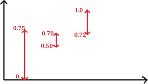The widest fuzzy interval solution can be seen for each quantity and their quality information can be seen in Figures 2–4. The total compartment representation is given in Figure 5.

Figure 2. Max-min fuzzy interval solution of the interest rate (${\mathbb{I}}_1$).

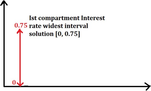
Figure 3. Max-min fuzzy interval solution of the demand of investment (${\mathbb{I}}_2$).

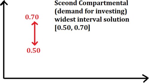
Figure 4. Max-min fuzzy interval solution of the price of index (${\mathbb{I}}_3$)

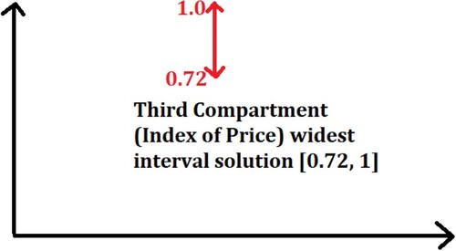
Figure 5. Max-min fuzzy interval solution of all the three compartments (${\mathbb{I}}_1,{\mathbb{I}}_2,{\mathbb{I}}_3$).

6. Conclusion

In the presented article, we explore the concept of the max-min fuzzy optimal interval solution within the context of oscillation or fluctuation observed in a business system modelled as a peer-to-peer educational network. The range of oscillation is determined by the two extreme values of the interval solution for each compartment of the system. This analysis proves to be highly suitable for studying systems involving variables such as the interest rate, demand for investment, and index of prices, which exhibit fluctuations in both quality and quantity. To optimize the oscillation range, we introduce the technique of the fluctuated wide solution in the form of an interval for the three agents within the system. A systematic procedure is established, incorporating theorems and lemmas, to compute the optimal widest and fluctuated solution for the considered system. Additionally, a numerical example is provided to illustrate the resolution process involved in this technique. This approach can be extended in the future to address real-life problems where fluctuations occur in both the quality and quantity of a given system, along with their associated information.

Disclosure statement

No potential conflict of interest was reported by the author(s).

Additional information

Funding

Conventional Project for 2022 in the “14th Five Year Plan” of Philosophy and Social Sciences in Guangdong Province [grant number GD22CJY24], 2022 Guangdong Province Key Construction Discipline Scientific Research Capacity Improvement Project [grant number 2022ZDJS062], Guangdong Provincial Key Laboratory of Functional Substances in Medicinal Edible Resources and Healthcare Products [grant number 2021B1212040015].

References

- Myšková H, Plavka J. On the solvability of interval max-min matrix equations. Linear Algebra Appl. 2020;590:85–96. doi: 10.1016/j.laa.2019.12.017
- Nitica V, Sergeev S. On the dimension of max–min convex sets. Fuzzy Sets Syst. 2015;271:88–101. doi: 10.1016/j.fss.2014.10.008
- Myšková H, Plávka J. AE and EA robustness of interval circulant matrices in max-min algebra. Fuzzy Sets Syst. 2020;384:91–104. doi: 10.1016/j.fss.2019.02.016
- Gavalec M, Plávka J. Simple image set of linear mappings in a max–min algebra. Discrete Appl Math. 2007;155(5):611–622. doi: 10.1016/j.dam.2006.08.011
- Li P, Fang S-C. On the resolution and optimization of a system of fuzzy relational equations with sup-T composition. Fuzzy Optim Decis Mak. 2008;7:169–214. doi: 10.1007/s10700-008-9029-y
- Dai H, Wang M, Yi X, et al. Secure max/min queries in two-tiered wireless sensor networks. IEEE Access. 2017;5:14478–14489. doi: 10.1109/ACCESS.2017.2731819
- Zheng J, Gao L, Zhang H, et al. Joint energy management and interference coordination with max-min fairness in ultra-dense HetNets. IEEE Access. 2018;6:32588–32600. doi: 10.1109/ACCESS.2018.2841989
- Zheng H, Li H, Hou S, et al. Joint resource allocation with weighted max-min fairness for NOMA-enabled v2X communications. IEEE Access. 2018;6:65449–65462. doi: 10.1109/ACCESS.2018.2877199
- Cantos L, Kim YH. Max-min fair energy beamforming for wireless powered communication with non-linear energy harvesting. IEEE Access. 2019;7:69516–69523. doi: 10.1109/Access.6287639
- Liu G, Deng H, Qian X, et al. Joint pilot allocation and power control to enhance max-min spectral efficiency in TDD massive MIMO systems. IEEE Access. 2019;7:149191–149201. doi: 10.1109/Access.6287639
- Sanchez E. Resolution of composite fuzzy relation equations. Inf Control. 1976;30(1):38–48. doi: 10.1016/S0019-9958(76)90446-0
- Sanchez E. Solutions in composite fuzzy relation equation, application to medical diagnosis in Brouwerian logic. Gupta MM, Saridis GN, Gaines BR, editors. Fuzzy Automata and Decision Process; 1977.
- Klir G, Yuan B. Fuzzy sets and fuzzy logic. Vol. Hoboken (NJ): Prentice Hall; 1995.
- Nobuhara H, Bede B, Hirota K. On various eigen fuzzy sets and their application to image reconstruction. Inf Sci (Ny). 2006;176(20):2988–3010. doi: 10.1016/j.ins.2005.11.008
- Nobuhara H, Pedrycz W, Hirota K. Fast solving method of fuzzy relational equation and its application to lossy image compression/reconstruction. IEEE Trans Fuzzy Syst. 2000;8(3):325–334. doi: 10.1109/91.855920
- Di Nola A, Sessa S, Pedrycz W, et al. Fuzzy relation equations and their applications to knowledge engineering. Vol. Springer Science & Business Media; 2013.
- Lee H-C, Guu S-M. On the optimal three-tier multimedia streaming services. Fuzzy Optim Decis Mak. 2003;2:31–39. doi: 10.1023/A:1022848114005
- Yang X-P, Zhou X-G, Cao B-Y. Single-variable term semi-latticized fuzzy relation geometric programming with max-product operator. Inf Sci (Ny). 2015;325:271–287. doi: 10.1016/j.ins.2015.07.015
- Li J-X, Yang SJ. Fuzzy relation inequalities about the data transmission mechanism in bittorrent-like peer-to-peer file sharing systems. In: 2012 9th International Conference on Fuzzy Systems and Knowledge Discovery, IEEE; 2012. p. 452-456.
- Yang X-P, Zhou X-G, Cao B-Y. Min-max programming problem subject to addition-min fuzzy relation inequalities. IEEE Trans Fuzzy Syst. 2015;24(1):111–119. doi: 10.1109/TFUZZ.2015.2428716
- Yang X-P. Optimal-vector-based algorithm for solving min-max programming subject to addition-min fuzzy relation inequality. IEEE Trans Fuzzy Syst. 2016;25(5):1127–1140. doi: 10.1109/TFUZZ.91
- Chiu Y-L, Guu S-M, Yu J, et al. A single-variable method for solving min–max programming problem with addition-min fuzzy relational inequalities. Fuzzy Optim Decis Mak. 2019;18:433–449. doi: 10.1007/s10700-019-09305-9
- Guu S-M, Yu J, Wu Y-K. A two-phase approach to finding a better managerial solution for systems with addition-min fuzzy relational inequalities. IEEE Trans Fuzzy Syst. 2017;26(4):2251–2260. doi: 10.1109/TFUZZ.2017.2771406
- Guu S-M, Wu Y-K. Multiple objective optimization for systems with addition–min fuzzy relational inequalities. Fuzzy Optim Decis Mak. 2019;18(4):529–544. doi: 10.1007/s10700-019-09306-8
- Guo F-F, Shen J. A smoothing approach for minimizing a linear function subject to fuzzy relation inequalities with addition–min composition. Int J Fuzzy Syst. 2019;21:281–290. doi: 10.1007/s40815-018-0530-3
- Molai AA. Fuzzy linear objective function optimization with fuzzy-valued max-product fuzzy relation inequality constraints. Math Comput Model. 2010;51(9-10):1240–1250. doi: 10.1016/j.mcm.2010.01.006
- Molai AA. The quadratic programming problem with fuzzy relation inequality constraints. Comput Ind Eng. 2012;62(1):256–263. doi: 10.1016/j.cie.2011.09.012
- Molai AA. A new algorithm for resolution of the quadratic programming problem with fuzzy relation inequality constraints. Comput Ind Eng. 2014;72:306–314. doi: 10.1016/j.cie.2014.03.024
- Yang X-P, Cao B-Y, Zhou X-G. Latticized linear programming subject to max-product fuzzy relation inequalities with application in wireless communication. Inf Sci (Ny). 2016;358:44–55. doi: 10.1016/j.ins.2016.04.014
- Yang X-P, Yuan D-H, Cao B-Y. Lexicographic optimal solution of the multi-objective programming problem subject to max-product fuzzy relation inequalities. Fuzzy Sets Syst. 2018;341:92–112. doi: 10.1016/j.fss.2017.08.001
- Xiao G, Zhu T, Chen Y, et al. Linear searching method for solving approximate solution to system of max-min fuzzy relation equations with application in the instructional information resources allocation. IEEE Access. 2019;7:65019–65028. doi: 10.1109/Access.6287639
- Yang X-P. Evaluation model and approximate solution to inconsistent max-min fuzzy relation inequalities in P2P file sharing system. Complexity. 2019;2019. doi: 10.1155/2019/6901818
- Jiang X, Li J, Li B, et al. Bifurcation, chaos, and circuit realisation of a new four-dimensional memristor system. Int J Nonlinear Sci Numer Simul. 2022;0. doi: 10.1515/ijnsns-2021-0393
- Li B, Eskandari Z. Dynamical analysis of a discrete-time SIR epidemic model. J Franklin Inst. 2023;360(12):7989–8007. doi: 10.1016/j.jfranklin.2023.06.006
- Li B, Eskandari Z, Avazzadeh Z. Dynamical behaviors of an SIR epidemic model with discrete time. Fractal Fract. 2022;6(11):659. doi: 10.3390/fractalfract6110659
- Li B, Eskandari Z, Avazzadeh Z. Strong resonance bifurcations for a discrete-time prey–predator model. J Appl Math Comput. 2023;69:2421–2438.
- He Q, Zhang X, Xia P, et al. A comparison research on dynamic characteristics of Chinese and American energy prices. J Global Inf Manage (JGIM). 2023;31(1):1–16. doi: 10.4018/JGIM
- Li B, Zhang T, Zhang C. Investigation of financial bubble mathematical model under fractal-fractional caputo derivative. FRACTALS (fractals). 2023;31(05):1–13.
- Chen WC. Nonlinear dynamics and chaos in a fractional-order financial system. Chaos Solitons Fractals. 2008;36(5):1305–1314. doi: 10.1016/j.chaos.2006.07.051
- Wang PZ, Zhang DZ, Sanchez E, et al. Latticized linear programming and fuzzy relation inequalities. J Math Anal Appl. 1991;159(1):72–87. doi: 10.1016/0022-247X(91)90222-L
- Guo F-F, Pang L-P, Meng D, et al. An algorithm for solving optimization problems with fuzzy relational inequality constraints. Inf Sci (Ny). 2013;252:20–31. doi: 10.1016/j.ins.2011.09.030
- Fang S-C, Li G. Solving fuzzy relation equations with a linear objective function. Fuzzy Sets Syst. 1999;103(1):107–113. doi: 10.1016/S0165-0114(97)00184-X
- Yang X-P. Linear programming method for solving semi-latticized fuzzy relation geometric programming with max-min composition. Int J Uncertain Fuzz Knowledge-Based Syst. 2015;23(05):781–804. doi: 10.1142/S0218488515500348