Solution of local fractional generalized coupled Korteweg–de Vries (cKdV) equation using local fractional homotopy analysis method and Adomian decomposition method

ABSTRACT

In this study, time-fractional coupled Korteweg–de Vries (cKdV) equations are solved using an efficient and reliable numerical technique. The classical cKdV system has been generalized into the time-fractional cKdV system. We employ the local fractional homotopy analysis method (LFHAM) and the Adomian decomposition method (ADM) to propose an approximate solution for fractional cKdV equations. Both approaches determined findings are compared together. The findings clearly demonstrate that the suggested methods are appropriate and efficient for handling both linear and nonlinear issues in engineering and sciences. To demonstrate the suggested approaches' competencies, examples are provided. Convergent series form has been used to make the solutions. The relevance of the techniques is illustrated through graphic representations of the solution.

KEYWORDS:

• Local fractional derivative
• coupled Korteweg–de Vries equation
• homotopy analysis method
• Adomian decomposition method

2010 MATHEMATICS SUBJECT CLASSIFICATIONS:

• 34A34
• 65M06
• 26A33

1. Introduction

Real-life problem of engineering and sciences gives rise to nonlinear ordinary differential equations ( ODEs) and partial differential equations ( PDEs). Non-linear system has varied range of engineering applications. Most of the real-life problems are convertible into nonlinear mathematical models. Therefore, resolving such a system has its significance and demands in-depth research. Researchers are motivated to develop and investigated effective methods and techniques to solve such dynamical systems, which exhibit nonlinearities. Yang et al. have shown nonlinear dynamics for local fractional Burger equation arising in fractal flow [1], similarly, Yang, Gao and Srivastava have worked for non-differentiable exact solutions for the nonlinear ODEs defined on fractal sets [2] and Dubey and Goswami have solved the nonlinear diffusion equation [3]. In this regard, time-dependent nonlinear coupled Korteweg–de Vries (cKdV) equations attracted a lot of study interest. Apart from the nonlinear system, we see frequent presence of ODEs, PDEs of fractional order in many fields like fluid dynamics, biology and physics. Numerous disciplines, including mechanics, electrical, chemistry, biology and economics, particularly control theory, signal image processing and groundwater issues, have benefited greatly from the use of fractional calculus. Many phenomena occurred in engineering, physical and medical science problems can be described by fractional order ODEs, PDEs effectively. Khan et al. have worked for the numerical solution of advection–diffusion equations involving Atangana–Baleanu time fractional derivative [4], Baleanu et al. have worked on the mathematical modelling of human liver with Caputo–Fabrizio fractional derivative [5], Defterli et al. have solved problems related to accelerated mass-spring system by fractal treatment [6]. Many researchers have been working to find analytical approximate solution of local fractional PDEs [7–11].

Local fractional calculus operator is first introduced by Kolwankar and Gangal [12] which is established on the fractional derivative of Riemann–Lioville sense. Non-differentiate functions can be easily handled by above-mentioned operators. A lot of scholars have also worked on the development of the fractal fractional derivative; in addition to this, He et al. have given new promises and future challenges of fractal calculus from two scale thermodynamics to fractal variational principle [13].

Numerous numerical and analytical techniques have been used by researchers during the past 20 years to get analytical or approximate solutions of local fractional PDEs, such as the local fractional Laplace transform, local fractional variational iteration, local fractional homotopy perturbation, local fractional Laplace homotopy perturbation, local fractional reduced differential transform methods, Laplace variational iteration methods and so on. Dubey et al. have solved Klein–Gordon equations by using homotopy perturbation Mohand transform method [14], Yang et al. have used local fractional series expansion method to solve Klein–Gordon equations on Cantor sets [15], Wang et al. have applied local fractional function decomposition method for solving inhomogeneous wave equations with local fractional derivative [16]. Similarly many research works have been done in this context [17–21].

This study's main goal is to find a local fractional derivative solution to the generalized fractional cKdV equation.

Figure 1. Graphical representation of solution of Equation (19(19) $\begin{array}{rl}& \frac{{\mathrm{\partial }}^{\upsilon }\varphi }{\mathrm{\partial }{k}^{\upsilon }}+\frac{{\mathrm{\partial }}^{3\upsilon }\varphi }{\mathrm{\partial }{l}^{3\upsilon }}+2{\varphi }^n\frac{{\mathrm{\partial }}^{\upsilon }\varphi }{\mathrm{\partial }{l}^{\upsilon }}+2{\psi }^m\frac{{\mathrm{\partial }}^{\upsilon }\varphi }{\mathrm{\partial }{l}^{\upsilon }}=0,\end{array}$(19) ) for $\nu =0.5$.

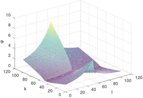
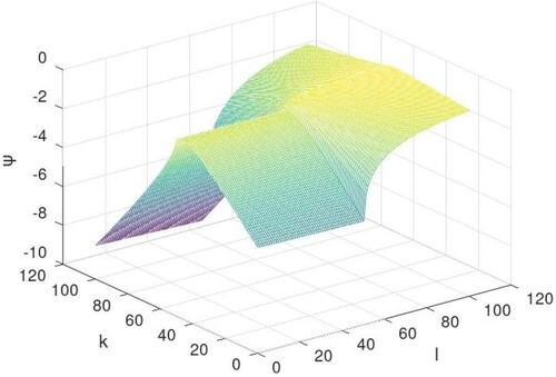
Figure 2. Graphical representation of solution of Equation (19(19) $\begin{array}{rl}& \frac{{\mathrm{\partial }}^{\upsilon }\varphi }{\mathrm{\partial }{k}^{\upsilon }}+\frac{{\mathrm{\partial }}^{3\upsilon }\varphi }{\mathrm{\partial }{l}^{3\upsilon }}+2{\varphi }^n\frac{{\mathrm{\partial }}^{\upsilon }\varphi }{\mathrm{\partial }{l}^{\upsilon }}+2{\psi }^m\frac{{\mathrm{\partial }}^{\upsilon }\varphi }{\mathrm{\partial }{l}^{\upsilon }}=0,\end{array}$(19) ) for $\nu =0.8$.

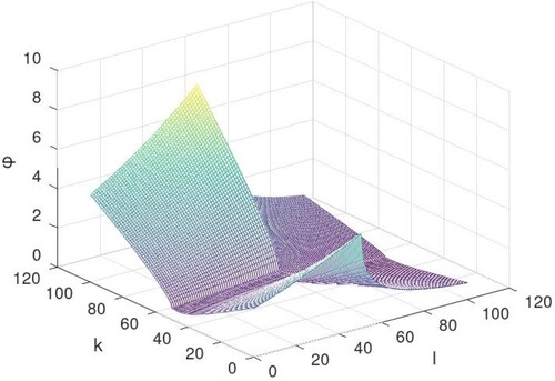
Figure 3. Graphical representation of solution of Equation (19(19) $\begin{array}{rl}& \frac{{\mathrm{\partial }}^{\upsilon }\varphi }{\mathrm{\partial }{k}^{\upsilon }}+\frac{{\mathrm{\partial }}^{3\upsilon }\varphi }{\mathrm{\partial }{l}^{3\upsilon }}+2{\varphi }^n\frac{{\mathrm{\partial }}^{\upsilon }\varphi }{\mathrm{\partial }{l}^{\upsilon }}+2{\psi }^m\frac{{\mathrm{\partial }}^{\upsilon }\varphi }{\mathrm{\partial }{l}^{\upsilon }}=0,\end{array}$(19) ) for $\nu =0.99$.

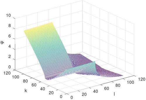
Figure 4. Graphical representation of solution of Equation (20(20) $\begin{array}{rl}& \frac{{\mathrm{\partial }}^{\upsilon }\psi }{\mathrm{\partial }{k}^{\upsilon }}+\frac{{\mathrm{\partial }}^{3\upsilon }\psi }{\mathrm{\partial }{l}^{3\upsilon }}+2{\psi }^n\frac{{\mathrm{\partial }}^{\upsilon }\psi }{\mathrm{\partial }{l}^{\upsilon }}+2{\varphi }^m\frac{{\mathrm{\partial }}^{\upsilon }\psi }{\mathrm{\partial }{l}^{\upsilon }}=0,\end{array}$(20) ) for $\nu =0.5$.

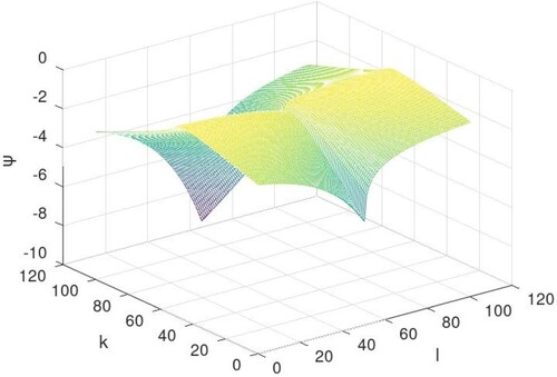
Figure 5. Graphical representation of solution of Equation (20(20) $\begin{array}{rl}& \frac{{\mathrm{\partial }}^{\upsilon }\psi }{\mathrm{\partial }{k}^{\upsilon }}+\frac{{\mathrm{\partial }}^{3\upsilon }\psi }{\mathrm{\partial }{l}^{3\upsilon }}+2{\psi }^n\frac{{\mathrm{\partial }}^{\upsilon }\psi }{\mathrm{\partial }{l}^{\upsilon }}+2{\varphi }^m\frac{{\mathrm{\partial }}^{\upsilon }\psi }{\mathrm{\partial }{l}^{\upsilon }}=0,\end{array}$(20) ) for $\nu =0.8$.

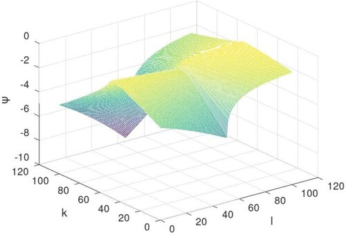
Figure 6. Graphical representation of Equation (20(20) $\begin{array}{rl}& \frac{{\mathrm{\partial }}^{\upsilon }\psi }{\mathrm{\partial }{k}^{\upsilon }}+\frac{{\mathrm{\partial }}^{3\upsilon }\psi }{\mathrm{\partial }{l}^{3\upsilon }}+2{\psi }^n\frac{{\mathrm{\partial }}^{\upsilon }\psi }{\mathrm{\partial }{l}^{\upsilon }}+2{\varphi }^m\frac{{\mathrm{\partial }}^{\upsilon }\psi }{\mathrm{\partial }{l}^{\upsilon }}=0,\end{array}$(20) ) for $\nu =0.99$.

In the exploration of nonlinear physical processes, the investigation of travelling wave solutions for the nonlinear system of equations is a vital step. The fluid flow beneath a pressure surface is visible along lakeshores and beaches as shallow water waves. For the past three decades, researchers have been working on a mathematical model of this phenomenon in a variety of science and engineering fields, including oceanography. For example, the long-wave short-wave interaction equation [22–26], the Kadomtsev–Petviashvili equation [24], the Gear–Grimshaw model [25] and the Schrödinger–Boussinesq equation [26] are some of the mathematical models that are presented in this context. To define a wide range of physical occurrences utilized to simulate the interaction and evolution of non-linear waves, the study of the KdV equation is important [27]. Waves on shallow water surfaces are quantitatively represented by the KdV equation. Boussinesq first presented the KdV equation in 1877, and Diederik Korteweg and Gustav de Vries later rediscovered it (1895) [28].

Now, we write fractional-order KdV equation: (1) $D_t^{\alpha }v+v^n{D}_x^{\alpha }v+D_x^{3\alpha }v=0,t>0,\alpha <1.$(1) This research work is a good discussion on the solution of nonlinear fractional cKdV equation. Hirota and Satsums introduced the cKdV equation in 1981. They discussed the interaction of two long waves with different dispersion relations [29].

The function of trigonometric transform approach, the F-expansion approach, the homotopy perturbation as well as its transformation approach, and the Adomian decomposition method (ADM) are the primary methods that have been used by various authors to solve coupled equations [30, 31]. Furthermore, the local fractional reduced differential transform and local fractional Laplace variational iteration methods were also used by Jafari et al. [32, 33] to find approximations of solutions for cKdV equations.

They have solved the following system of fractional cKdV equations: (2) $\begin{array}{rl}& \frac{{\mathrm{\partial }}^{\upsilon }\varphi }{\mathrm{\partial }{k}^{\upsilon }}+\frac{{\mathrm{\partial }}^{3\upsilon }\varphi }{\mathrm{\partial }{l}^{3\upsilon }}+2\varphi \frac{{\mathrm{\partial }}^{\upsilon }\varphi }{\mathrm{\partial }{l}^{\upsilon }}+2\psi \frac{{\mathrm{\partial }}^{\upsilon }\varphi }{\mathrm{\partial }{l}^{\upsilon }}=0,\end{array}$(2) (3) $\begin{array}{rl}& \frac{{\mathrm{\partial }}^{\upsilon }\psi }{\mathrm{\partial }{k}^{\upsilon }}+\frac{{\mathrm{\partial }}^{3\upsilon }\psi }{\mathrm{\partial }{l}^{3\upsilon }}+2\psi \frac{{\mathrm{\partial }}^{\upsilon }\psi }{\mathrm{\partial }{l}^{\upsilon }}+2\varphi \frac{{\mathrm{\partial }}^{\upsilon }\psi }{\mathrm{\partial }{l}^{\upsilon }}=0.\end{array}$(3)

Due to its frequent occurrence in numerous real-world problems, nonlinear cKdV equations have been the subject of many research studies; therefore, understanding its generalized form is significant. In this research, authors investigate the most general kind of coupled nonlinear fractional KdV equation.

Consider the following the n-generalized fractional cKdV equation: (4) $\begin{array}{rl}& \frac{{\mathrm{\partial }}^{\upsilon }\varphi }{\mathrm{\partial }{k}^{\upsilon }}+\frac{{\mathrm{\partial }}^{3\upsilon }\varphi }{\mathrm{\partial }{l}^{3\upsilon }}+2{\varphi }^n\frac{{\mathrm{\partial }}^{\upsilon }\varphi }{\mathrm{\partial }{l}^{\upsilon }}+2{\psi }^m\frac{{\mathrm{\partial }}^{\upsilon }\varphi }{\mathrm{\partial }{l}^{\upsilon }}=0,\end{array}$(4) (5) $\begin{array}{rl}& \frac{{\mathrm{\partial }}^{\upsilon }\psi }{\mathrm{\partial }{k}^{\upsilon }}+\frac{{\mathrm{\partial }}^{3\upsilon }\psi }{\mathrm{\partial }{l}^{3\upsilon }}+2{\psi }^n\frac{{\mathrm{\partial }}^{\upsilon }\psi }{\mathrm{\partial }{l}^{\upsilon }}+2{\varphi }^m\frac{{\mathrm{\partial }}^{\upsilon }\psi }{\mathrm{\partial }{l}^{\upsilon }}=0,\end{array}$(5) with initial conditions $\varphi \left(l,0\right)={\varphi }_0\left(l\right)$, $\psi \left(l,0\right)={\psi }_0\left(l\right)$.

In the present paper, authors suggest two approaches to produce analytical approximate solution for generalized fractional cKdV equations, with initial conditions $\varphi \left(l,0\right)=E_{\upsilon }\left(-l^{\upsilon }\right),\psi \left(l,0\right)=-E_{\upsilon }\left(-l^{\upsilon }\right).$

The focus of this study is on the fractional cKdV equations and the use of the ADM and local fractional homotopy analysis method (LFHAM). Numerous problems in the real world, including those involving magma movement, surface waves, Rossby waves, internal waves in a fluid with stratified density, and plasma waves, depend on the KdV equation. Maitama and Zhao introduced the local homotopy analysis method initially [34], LFHAM is a very helpful tool for solving the differential equations. By carefully choosing the parameters h and H, this approach LFHAM is particularly effective in regulating and controlling the convergence of the solution [35].

A numerical technique based on Adomian's invention [36] of the ADM is presented in this study as an approximate method for solving fractional cKdV equations. The ADM is a potent method that offers effective algorithms for approximate analytical answers and numerical simulations for practical applications in applied sciences and engineering [37, 38].

Both approaches are excellent techniques for solving generalized nonlinear fractional differential equations, even though the outcome is expressed in terms of an infinite series. The method's drawback is that numerous terms from the infinite series must be taken into account to obtain high accuracy. To develop an analytical approximate solution for local fractional PDEs, numerous scholars have been working [39–42].

Definition 1.1

The local fractal derivative for a real-valued function, L at $g=g_0$ is defined as [43, 44] $\begin{array}{rl}{D}^{\text{β}}L\left(g_0\right)& =\frac{d^{\text{β}}}{\mathrm{d}{g}^{\text{β}}}L\left(g\right){|}_{g_0}\\ & =\underset{g\to g_0}{lim}\frac{{\mathrm{\Delta }}^{\text{β}}\left(L\left(g\right)-L\left(g_0\right)\right)}{{\left(g-g_0\right)}^{\text{β}}},\end{array}$such that $|L\left(g\right)-L_0\left(g\right)|<{\in }^{\text{β}},$where ${\mathrm{\Delta }}^{\text{β}}\left(L\left(g\right)-L\left(g_0\right)\right)\cong \left[L\left(g\right)-L\left(g_0\right)\right]\mathrm{\Gamma }\left(1+\text{β}\right).$

This paper is organized as follows:

Section 1:	Introduction
Section 2:	Existence and Oneness of the Solution
Section 3:	Analysis of the methods and applications
Section 4:	Conclusion

2. Existence and oneness of the solution

N-generalized fractional cKdV equations are given as follows: (6) $\{\begin{array}{l}\frac{{\mathrm{\partial }}^{\upsilon }\varphi }{\mathrm{\partial }{\lambda }^{\upsilon }}+\frac{{\mathrm{\partial }}^{3\upsilon }\varphi }{\mathrm{\partial }{\hslash }^{3\upsilon }}+2{\varphi }^n\frac{{\mathrm{\partial }}^{\upsilon }\varphi }{\mathrm{\partial }{\hslash }^{\upsilon }}+2{\psi }^m\frac{{\mathrm{\partial }}^{\upsilon }\varphi }{\mathrm{\partial }{\hslash }^{\upsilon }}=f(\hslash ,\lambda ),\\ \frac{{\mathrm{\partial }}^{\upsilon }\psi }{\mathrm{\partial }{\lambda }^{\upsilon }}+\frac{{\mathrm{\partial }}^{3\upsilon }\psi }{\mathrm{\partial }{\hslash }^{3\upsilon }}+2{\psi }^n\frac{{\mathrm{\partial }}^{\upsilon }\psi }{\mathrm{\partial }{\hslash }^{\upsilon }}+2{\varphi }^m\frac{{\mathrm{\partial }}^{\upsilon }\psi }{\mathrm{\partial }{\hslash }^{\upsilon }}=p(\hslash ,\lambda ),\end{array}$(6) with $\begin{array}{rl}\varphi \left(\hslash ,0\right)& =F\left(\hslash \right),\\ \psi \left(\hslash ,0\right)& =P\left(\hslash \right),\end{array}$system (6(6) $\{\begin{array}{l}\frac{{\mathrm{\partial }}^{\upsilon }\varphi }{\mathrm{\partial }{\lambda }^{\upsilon }}+\frac{{\mathrm{\partial }}^{3\upsilon }\varphi }{\mathrm{\partial }{\hslash }^{3\upsilon }}+2{\varphi }^n\frac{{\mathrm{\partial }}^{\upsilon }\varphi }{\mathrm{\partial }{\hslash }^{\upsilon }}+2{\psi }^m\frac{{\mathrm{\partial }}^{\upsilon }\varphi }{\mathrm{\partial }{\hslash }^{\upsilon }}=f(\hslash ,\lambda ),\\ \frac{{\mathrm{\partial }}^{\upsilon }\psi }{\mathrm{\partial }{\lambda }^{\upsilon }}+\frac{{\mathrm{\partial }}^{3\upsilon }\psi }{\mathrm{\partial }{\hslash }^{3\upsilon }}+2{\psi }^n\frac{{\mathrm{\partial }}^{\upsilon }\psi }{\mathrm{\partial }{\hslash }^{\upsilon }}+2{\varphi }^m\frac{{\mathrm{\partial }}^{\upsilon }\psi }{\mathrm{\partial }{\hslash }^{\upsilon }}=p(\hslash ,\lambda ),\end{array}$(6) ) can be written as (7) $\{\begin{array}{l}{L}_{\nu }\left[\varphi \left(\hslash ,\lambda \right)\right]=\rho \left[\varphi \left(\hslash ,\lambda \right)\right],\\ L_{\nu }\left[\psi \left(\hslash ,\lambda \right)\right]=\rho \left[\psi \left(\hslash ,\lambda \right)\right],\end{array}$(7) with $\begin{array}{rl}\varphi \left(\hslash ,0\right)& ={\varphi }_0\left(\hslash \right),\\ \psi \left(\hslash ,0\right)& ={\psi }_0\left(\hslash \right),\end{array}$where (8) $\begin{array}{rl}\rho \left[\varphi \left(\hslash ,\lambda \right)\right]& =F\left(\hslash ,\lambda \right)-{{\varphi }_l}^{3\nu }-2{\varphi }^m{\varphi }_{\hslash }^{\nu }-2{\psi }^m{\varphi }_{\hslash }^{\nu },\end{array}$(8) (9) $\begin{array}{rl}\rho \left[\psi \left(\hslash ,\lambda \right)\right]& =P\left(\hslash ,\lambda \right)-{{\psi }_l}^{3\nu }-2{\psi }^m{\psi }_{\hslash }^{\nu }-2{\varphi }^m{\psi }_{\hslash }^{\nu }.\end{array}$(9)

Theorem 2.1

Let $\rho \left[\varphi \left(\hslash ,\lambda \right)\right]$ defined by (8(8) $\begin{array}{rl}\rho \left[\varphi \left(\hslash ,\lambda \right)\right]& =F\left(\hslash ,\lambda \right)-{{\varphi }_l}^{3\nu }-2{\varphi }^m{\varphi }_{\hslash }^{\nu }-2{\psi }^m{\varphi }_{\hslash }^{\nu },\end{array}$(8) ) is local fractional continuous and satisfies Lipschitz condition, i.e. (10) $\begin{array}{rl}& \left|\rho \left[{\varphi }_1\right(\hslash ,\lambda \left)\right]-\rho \left[{\varphi }_2\right(\hslash ,\lambda \left)\right]\right|\le {\eta }^{\nu }\left|{\varphi }_1(\hslash ,\lambda )-{\varphi }_2(\hslash ,\lambda )\right|,\\ & 0\le \nu \le 1,0<\eta <1.\end{array}$(10) Then the system $\begin{array}{rl}& \{\begin{array}{l}{L}_{\nu }\left[\varphi \left(\hslash ,\lambda \right)\right]=\rho \left[\varphi \left(\hslash ,\lambda \right)\right],\\ L_{\nu }\left[\psi \left(\hslash ,\lambda \right)\right]=\rho \left[\psi \left(\hslash ,\lambda \right)\right],\end{array}\\ & \varphi \left(\hslash ,0\right)={\varphi }_0\left(\hslash \right),\psi \left(\hslash ,0\right)={\psi }_0\left(\hslash \right),\end{array}$has a unique solution in $C_{\nu }[m,n]$, where $C_{\nu }$ is the space of a continuous function with fractal derivative of order ν.

Proof.

Let the map $\tau :C_{\nu }[m,n]\to C_{\nu }[m,n]$ be defined by (11) $\tau \left[\varphi \right(\hslash ,\lambda \left)\right]={\varphi }_0\left(\hslash \right)+\frac{1}{\mathrm{\Gamma }\left(1+\nu \right)}{\int }_{\nu }^{\text{β}}\rho \left[\varphi \right(\hslash ,s\left)\right](\mathrm{d}s{)}^{\nu }$(11) First, authors establish by induction that (12) $\begin{array}{rl}& {\Vert {\tau }^p\left\{{\varphi }_1\left(\left(\hslash ,\lambda \right)\right)\right\}-{\tau }^p\left\{{\varphi }_2\left(\left(\hslash ,\lambda \right)\right)\right\}\Vert }_{\nu }\le {\frac{{\eta }^{p\nu }\left|n^{\nu }-m^{\nu }\right|}{{\mathrm{\Gamma }}^p\left(1+\nu \right)}}^p{\Vert {\varphi }_1\left(\left(\hslash ,\lambda \right)\right)-{\varphi }_2\left(\left(\hslash ,\lambda \right)\right)\Vert }_{\nu },\\ & p=1,2,3,\dots \end{array}$(12) for p = 1, one can get $\left|\tau \left\{{\varphi }_1\left(\hslash ,\lambda \right)\right\}-\tau \left\{{\varphi }_2\left(\hslash ,\lambda \right)\right\}\right|=\left|\frac{1}{\mathrm{\Gamma }\left(1+\nu \right)}{\int }_{\nu }^{\text{β}}\left(\rho \left\{{\varphi }_1\left(\hslash ,s\right)\right\}-\rho \left\{{\varphi }_2\left(\hslash ,s\right)\right\}\right){\left(\mathrm{d}s\right)}^{\nu }\right|$or (13) $\begin{array}{rl}& \left|\tau \left\{{\varphi }_1\left(\hslash ,\lambda \right)\right\}-\tau \left\{{\varphi }_2\left(\hslash ,\lambda \right)\right\}\right|\le \left|\frac{1}{\mathrm{\Gamma }\left(1+\nu \right)}{\int }_{\nu }^{\text{β}}{\eta }^{\nu }\left|\left\{{\varphi }_1\left(\hslash ,s\right)\right\}-\left\{{\varphi }_2\left(\hslash ,s\right)\right\}\right|{\left(\mathrm{d}s\right)}^{\nu }\right|,\\ & \left|\tau \left\{{\varphi }_1\left(\hslash ,\lambda \right)\right\}-\tau \left\{{\varphi }_2\left(\hslash ,\lambda \right)\right\}\right|\le \frac{{\eta }^{\nu }\left|n^{\nu }-m^{\nu }\right|}{\mathrm{\Gamma }\left(1+\nu \right)}{\Vert {\varphi }_1\left(\hslash ,\lambda \right)-{\varphi }_2\left(\hslash ,\lambda \right)\Vert }_{\nu }.\end{array}$(13) This implies that (14) ${\Vert \tau \left\{{\varphi }_1\left(\hslash ,\lambda \right)\right\}-\tau \left\{{\varphi }_2\left(\hslash ,\lambda \right)\right\}\Vert }_{\nu }\le \frac{{\eta }^{\nu }\left|n^{\nu }-m^{\nu }\right|}{\mathrm{\Gamma }\left(1+\nu \right)}{\Vert {\varphi }_1\left(\hslash ,\lambda \right)-{\varphi }_2\left(\hslash ,\lambda \right)\Vert }_{\nu },$(14) assume the equality holds for p = j (15) ${\Vert {\tau }^j\left\{{\varphi }_1\left(\hslash ,\lambda \right)\right\}-{\tau }^j\left\{{\varphi }_2\left(\hslash ,\lambda \right)\right\}\Vert }_{\nu }\le \frac{{\eta }^{j\nu }{\left|n^{\nu }-m^{\nu }\right|}^j}{{\mathrm{\Gamma }}^j\left(1+\nu \right)}{\Vert {\varphi }_1\left(\hslash ,\lambda \right)-{\varphi }_2\left(\hslash ,\lambda \right)\Vert }_{\nu },$(15) for p = j + 1, consider $\begin{array}{rl}& {\Vert {\tau }^{j+1}\left\{{\varphi }_1\left(\hslash ,\lambda \right)\right\}-{\tau }^{j+1}\left\{{\varphi }_2\left(\hslash ,\lambda \right)\right\}\Vert }_{\nu }\\ & =\left|\frac{1}{\mathrm{\Gamma }\left(1+\nu \right)}{\int }_{\nu }^{\text{β}}\rho \left[{\tau }^j\left\{{\varphi }_1\left(\hslash ,s\right)\right\}\right]-\rho \left[{\tau }^k\left\{{\varphi }_2\left(\hslash ,s\right)\right\}\right]{\left(\mathrm{d}s\right)}^{\nu }\right|\end{array}$further it can be written as $\begin{array}{rl}& {\Vert {\tau }^{j+1}\left\{{\varphi }_1\left(\hslash ,\lambda \right)\right\}-{\tau }^{j+1}\left\{{\varphi }_2\left(\hslash ,\lambda \right)\right\}\Vert }_{\nu }\\ & \le \left|\frac{1}{\mathrm{\Gamma }\left(1+\nu \right)}{\int }_{\nu }^{\text{β}}{\eta }^{\nu }\left|{\tau }^j\left\{{\varphi }_1\left(\hslash ,s\right)\right\}-{\tau }^j\left\{{\varphi }_2\left(\hslash ,s\right)\right\}\right|\mathrm{d}{s}^{\nu }\right|.\end{array}$Therefore, (16) ${\Vert {\tau }^{j+1}\left\{{\varphi }_1\left(\hslash ,\lambda \right)\right\}-{\tau }^{j+1}\left\{{\varphi }_2\left(\hslash ,\lambda \right)\right\}\Vert }_{\nu }\le \frac{{\eta }^{(j+1)\nu }{\left|n^{\nu }-m^{\nu }\right|}^{j+1}}{{\mathrm{\Gamma }}^{(j+1)}\left(1+\nu \right)}{\Vert {\varphi }_1\left(\hslash ,\lambda \right)-{\varphi }_2\left(\hslash ,\lambda \right)\Vert }_{\nu },$(16) hence, it proves our assumptions.

Now, we have (17) $\frac{{\eta }^{(j+1)\nu }{\left|n^{\nu }-m^{\nu }\right|}^{j+1}}{{\mathrm{\Gamma }}^{(j+1)}\left(1+\nu \right)}{\Vert {\varphi }_1\left(\hslash ,\lambda \right)-{\varphi }_2\left(\hslash ,\lambda \right)\Vert }_{\nu }\to 0,$(17) as $p\to \mathrm{\infty }$.

Similarly, one can write (18) $\frac{{\eta }^{(j+1)\nu }{\left|n^{\nu }-m^{\nu }\right|}^{j+1}}{{\mathrm{\Gamma }}^{(j+1)}\left(1+\nu \right)}{\Vert {\psi }_1\left(\hslash ,\lambda \right)-{\psi }_2\left(\hslash ,\lambda \right)\Vert }_{\nu }\to 0,$(18) as $p\to \mathrm{\infty }$.

Therefore system persists a unique solution.

3. Analysis of the methods and applications

Here, authors provide a quick overview of the techniques and applied to n-generalized cKdV equations.

3.1. The local fractional homotopy analysis method

Consider the following generalized fractional cKdV equations: (19) $\begin{array}{rl}& \frac{{\mathrm{\partial }}^{\upsilon }\varphi }{\mathrm{\partial }{k}^{\upsilon }}+\frac{{\mathrm{\partial }}^{3\upsilon }\varphi }{\mathrm{\partial }{l}^{3\upsilon }}+2{\varphi }^n\frac{{\mathrm{\partial }}^{\upsilon }\varphi }{\mathrm{\partial }{l}^{\upsilon }}+2{\psi }^m\frac{{\mathrm{\partial }}^{\upsilon }\varphi }{\mathrm{\partial }{l}^{\upsilon }}=0,\end{array}$(19) (20) $\begin{array}{rl}& \frac{{\mathrm{\partial }}^{\upsilon }\psi }{\mathrm{\partial }{k}^{\upsilon }}+\frac{{\mathrm{\partial }}^{3\upsilon }\psi }{\mathrm{\partial }{l}^{3\upsilon }}+2{\psi }^n\frac{{\mathrm{\partial }}^{\upsilon }\psi }{\mathrm{\partial }{l}^{\upsilon }}+2{\varphi }^m\frac{{\mathrm{\partial }}^{\upsilon }\psi }{\mathrm{\partial }{l}^{\upsilon }}=0,\end{array}$(20) with initial conditions $\varphi \left(l,0\right)={\varphi }_0\left(l\right)$ , $\psi \left(l,0\right)={\psi }_0\left(l\right)$.

Authors apply LFHAM to Equations (19(19) $\begin{array}{rl}& \frac{{\mathrm{\partial }}^{\upsilon }\varphi }{\mathrm{\partial }{k}^{\upsilon }}+\frac{{\mathrm{\partial }}^{3\upsilon }\varphi }{\mathrm{\partial }{l}^{3\upsilon }}+2{\varphi }^n\frac{{\mathrm{\partial }}^{\upsilon }\varphi }{\mathrm{\partial }{l}^{\upsilon }}+2{\psi }^m\frac{{\mathrm{\partial }}^{\upsilon }\varphi }{\mathrm{\partial }{l}^{\upsilon }}=0,\end{array}$(19) ) and (20(20) $\begin{array}{rl}& \frac{{\mathrm{\partial }}^{\upsilon }\psi }{\mathrm{\partial }{k}^{\upsilon }}+\frac{{\mathrm{\partial }}^{3\upsilon }\psi }{\mathrm{\partial }{l}^{3\upsilon }}+2{\psi }^n\frac{{\mathrm{\partial }}^{\upsilon }\psi }{\mathrm{\partial }{l}^{\upsilon }}+2{\varphi }^m\frac{{\mathrm{\partial }}^{\upsilon }\psi }{\mathrm{\partial }{l}^{\upsilon }}=0,\end{array}$(20) ), $rth$-order deformation equations are given by (21) $\begin{array}{rl}& L_{\alpha }\left[{\varphi }_r\left(l,k\right)-{\chi }_r{\varphi }_{r-1}\left(l,k\right)\right]=\hslash H\left(x,t\right)R_r\left[{\varphi }_{r-1},l,k\right],\end{array}$(21) (22) $\begin{array}{rl}& L_{\alpha }\left[{\psi }_r\left(l,k\right)-{\chi }_r{\psi }_{r-1}\left(l,k\right)\right]=\hslash H\left(x,t\right)R_r\left[{\psi }_{r-1},l,k\right],\end{array}$(22) where (23) $R_r\left[{\varphi }_{r-1},l,k\right]=\frac{{\mathrm{\partial }}^{\upsilon }{\varphi }_r}{\mathrm{\partial }{k}^{\upsilon }}+\frac{{\mathrm{\partial }}^{3\upsilon }{\varphi }_r}{\mathrm{\partial }{l}^{3\upsilon }}+2{{\varphi }_r}^n\frac{{\mathrm{\partial }}^{\upsilon }{\varphi }_r}{\mathrm{\partial }{l}^{\upsilon }}+2{{\psi }_r}^m\frac{{\mathrm{\partial }}^{\upsilon }{\varphi }_r}{\mathrm{\partial }{l}^{\upsilon }}$(23) and (24) $R_r\left[{\psi }_{r-1},l,k\right]=\frac{{\mathrm{\partial }}^{\upsilon }{\psi }_r}{\mathrm{\partial }{k}^{\upsilon }}+\frac{{\mathrm{\partial }}^{3\upsilon }{\psi }_r}{\mathrm{\partial }{l}^{3\upsilon }}+2{{\psi }_r}^n\frac{{\mathrm{\partial }}^{\upsilon }{\psi }_r}{\mathrm{\partial }{l}^{\upsilon }}+2{{\varphi }_r}^m\frac{{\mathrm{\partial }}^{\upsilon }{\psi }_r}{\mathrm{\partial }{l}^{\upsilon }}.$(24) Let $H\left(x,t\right)=1$, therefore by Equations (21(21) $\begin{array}{rl}& L_{\alpha }\left[{\varphi }_r\left(l,k\right)-{\chi }_r{\varphi }_{r-1}\left(l,k\right)\right]=\hslash H\left(x,t\right)R_r\left[{\varphi }_{r-1},l,k\right],\end{array}$(21) ) and (22(22) $\begin{array}{rl}& L_{\alpha }\left[{\psi }_r\left(l,k\right)-{\chi }_r{\psi }_{r-1}\left(l,k\right)\right]=\hslash H\left(x,t\right)R_r\left[{\psi }_{r-1},l,k\right],\end{array}$(22) ), $rth$-order deformation will be (25) $\begin{array}{rl}{\varphi }_r\left(l,k\right)& =\left({\chi }_r+h\right){\varphi }_{r-1}\left(l,k\right)-\left({\chi }_r+h\right){\varphi }_{r-1}\left(l,0\right)\\ & +h{I_n}^{\left(\alpha \right)}\left[\frac{{\mathrm{\partial }}^{3\upsilon }{\varphi }_{r-1}}{\mathrm{\partial }{l}^{3\upsilon }}+2{{\varphi }_{r-1}}^n\frac{{\mathrm{\partial }}^{\upsilon }{\varphi }_{r-1}}{\mathrm{\partial }{l}^{\upsilon }}+2{\psi }_{r-1}^m\frac{{\mathrm{\partial }}^{\upsilon }{\varphi }_{r-1}}{\mathrm{\partial }{l}^{\upsilon }}\right]\end{array}$(25) and (26) $\begin{array}{rl}{\psi }_r\left(l,k\right)& =\left({\chi }_r+h\right){\psi }_{r-1}\left(l,k\right)-\left({\chi }_r+h\right){\psi }_{r-1}\left(l,0\right)\\ & +h{I_n}^{\left(\alpha \right)}\left[\frac{{\mathrm{\partial }}^{3\upsilon }{\psi }_{r-1}}{\mathrm{\partial }{l}^{3\upsilon }}+2{{\psi }_{r-1}}^n\frac{{\mathrm{\partial }}^{\upsilon }{\psi }_{r-1}}{\mathrm{\partial }{l}^{\upsilon }}+2{\varphi }_{r-1}^m\frac{{\mathrm{\partial }}^{\upsilon }{\psi }_{r-1}}{\mathrm{\partial }{l}^{\upsilon }}\right].\end{array}$(26) Let ${\varphi }_0\left(l,k\right)=\varphi \left(l,0\right)=E_{\upsilon }\left(-l^{\upsilon }\right)$ and ${\psi }_0\left(l,k\right)=\psi \left(l,0\right)=E_{\upsilon }\left(-l^{\upsilon }\right)$, put r = 1 in Equation (25(25) $\begin{array}{rl}{\varphi }_r\left(l,k\right)& =\left({\chi }_r+h\right){\varphi }_{r-1}\left(l,k\right)-\left({\chi }_r+h\right){\varphi }_{r-1}\left(l,0\right)\\ & +h{I_n}^{\left(\alpha \right)}\left[\frac{{\mathrm{\partial }}^{3\upsilon }{\varphi }_{r-1}}{\mathrm{\partial }{l}^{3\upsilon }}+2{{\varphi }_{r-1}}^n\frac{{\mathrm{\partial }}^{\upsilon }{\varphi }_{r-1}}{\mathrm{\partial }{l}^{\upsilon }}+2{\psi }_{r-1}^m\frac{{\mathrm{\partial }}^{\upsilon }{\varphi }_{r-1}}{\mathrm{\partial }{l}^{\upsilon }}\right]\end{array}$(25) ) (27) ${\varphi }_1\left(l,k\right)=+h{I_n}^{\left(\alpha \right)}\left[\frac{{\mathrm{\partial }}^{3\upsilon }{\varphi }_0}{\mathrm{\partial }{l}^{3\upsilon }}+2{{\varphi }_0}^n\frac{{\mathrm{\partial }}^{\upsilon }{\varphi }_0}{\mathrm{\partial }{l}^{\upsilon }}+2{{\psi }_0}^m\frac{{\mathrm{\partial }}^{\upsilon }{\varphi }_0}{\mathrm{\partial }{l}^{\upsilon }}\right]$(27) or (28) $\begin{array}{rl}{\varphi }_1\left(l,k\right)& =+h{I_n}^{\left(\upsilon \right)}\left[\begin{array}{l}-E_{\upsilon }\left(-l^{\upsilon }\right)+2{E^n}_{\upsilon }\left(-l^{\upsilon }\right)\left(-E_{\upsilon }\left(-l^{\upsilon }\right)\right)\\ +2(-1{)}^m{E^{m+1}}_{\upsilon }\left(-l^{\upsilon }\right)\end{array}\right],\end{array}$(28) (29) $\begin{array}{rl}{\varphi }_1\left(l,k\right)& =-h{E}_{\upsilon }\left(-l^{\upsilon }\right)\left[1+2{E^n}_{\upsilon }\left(-l^{\upsilon }\right)+2{E_{\upsilon }}^m(-1{)}^m\left(-l^{\upsilon }\right)\right]\frac{k^{\upsilon }}{\mathrm{\Gamma }(1+\upsilon )}.\end{array}$(29) Similarly, (30) ${\psi }_1\left(l,k\right)=-h{I}^{\left(\upsilon \right)}\left[E_{\upsilon }\left(-l^{\upsilon }\right)+2{\left(-1\right)}^n{E^n}_{\upsilon }\left(-l^{\upsilon }\right)E_{\upsilon }\left(-l^{\upsilon }\right)+2{E_{\upsilon }}^m\left(-l^{\upsilon }\right)\right]$(30) or (31) ${\psi }_1\left(l,k\right)=-h{I}^{\left(\upsilon \right)}\left[1+2{\left(-1\right)}^n{E^n}_{\upsilon }\left(-l^{\upsilon }\right)+2{E_{\upsilon }}^m\left(-l^{\upsilon }\right)\right]\frac{k^{\upsilon }}{\mathrm{\Gamma }(1+\upsilon )}.$(31) Now put r = 2 in Equation (25(25) $\begin{array}{rl}{\varphi }_r\left(l,k\right)& =\left({\chi }_r+h\right){\varphi }_{r-1}\left(l,k\right)-\left({\chi }_r+h\right){\varphi }_{r-1}\left(l,0\right)\\ & +h{I_n}^{\left(\alpha \right)}\left[\frac{{\mathrm{\partial }}^{3\upsilon }{\varphi }_{r-1}}{\mathrm{\partial }{l}^{3\upsilon }}+2{{\varphi }_{r-1}}^n\frac{{\mathrm{\partial }}^{\upsilon }{\varphi }_{r-1}}{\mathrm{\partial }{l}^{\upsilon }}+2{\psi }_{r-1}^m\frac{{\mathrm{\partial }}^{\upsilon }{\varphi }_{r-1}}{\mathrm{\partial }{l}^{\upsilon }}\right]\end{array}$(25) ) (32) ${\varphi }_2\left(l,k\right)=\left({\chi }_2+h\right){\varphi }_1\left(l,k\right)+h{I}^{\left(\upsilon \right)}\left[\frac{{\mathrm{\partial }}^{3\upsilon }{\varphi }_1}{\mathrm{\partial }{l}^{3\upsilon }}+2{{\varphi }_1}^n\frac{{\mathrm{\partial }}^{\upsilon }{\varphi }_1}{\mathrm{\partial }{l}^{\upsilon }}+2{{\psi }_1}^m\frac{{\mathrm{\partial }}^{\upsilon }{\varphi }_1}{\mathrm{\partial }{l}^{\upsilon }}\right],$(32) or ${\varphi }_2\left(l,k\right)=\left(1+h\right)\left[h{E}_{\upsilon }\left(-l^{\upsilon }\right)\frac{k^{\upsilon }}{\mathrm{\Gamma }(1+\upsilon )}\left\{1-2{E^n}_{\upsilon }\left(-l^{\upsilon }\right)+2E_{\upsilon }\left(-l^{\upsilon }\right)\right\}\right],$or (33) ${\varphi }_2=\left[\begin{array}{c}\left\{\begin{array}{l}{E}_{\nu }\left(-l^{\nu }\right)+2(n+1{)}^3{E}_{\nu }^{n+1}\left(-l^{\nu }\right)+\\ 2(-1{)}^n(m+1{)}^3{E}_{\nu }^{m+1}\left(-l^{\nu }\right)\end{array}\right\}\frac{k^{2\nu }}{\mathrm{\Gamma }(1+2\nu )}\\ \begin{array}{l}+2{\left\{2{(-1)}^n{E}_{\nu }^{m+1}\left(-l^{\nu }\right)+E_{\nu }\left(-l^{\nu }\right)+2E_{\nu }^{n+1}\left(-l^{\nu }\right)\right\}}^n\\ \left\{\begin{array}{l}-E_{\nu }\left(-l^{\nu }\right)-2(n+1)E_{\nu }^{n+1}\left(-l^{\nu }\right)-\\ 2(-1{)}^m(m+1){E_{\nu }}^{m+1}\left(-l^{\nu }\right)\end{array}\right\}\end{array}\\ \frac{k^{(n+2)\nu }}{\mathrm{\Gamma }(1+(n+2\left)\nu \right)}\frac{\mathrm{\Gamma }(1+(n+1\left)\nu \right)}{\mathrm{\Gamma }{(1+\nu )}^{n+1}}+\\ 2{\left\{\begin{array}{l}-E_{\nu }\left(-l^{\nu }\right)-2E_{\nu }^{m+1}\left(-l^{\nu }\right)-\\ 2(-1{)}^n{E_{\nu }}^{n+1}\left(-l^{\nu }\right)\end{array}\right\}}^m\\ \begin{array}{l}\left\{\begin{array}{l}-E_{\nu }\left(-l^{\nu }\right)-2(n+1)E_{\nu }^{n+1}\left(-l^{\nu }\right)-\\ 2(-1{)}^m(m+1){E_{\nu }}^{m+1}\left(-l^{\nu }\right)\end{array}\right\}\\ \frac{k^{(m+2)\nu }}{\mathrm{\Gamma }(1+(m+2\left)\nu \right)}\frac{\mathrm{\Gamma }(1+(m+1\left)\nu \right)}{\mathrm{\Gamma }{(1+\nu )}^{m+1}}\end{array}\end{array}\right]$(33) Similarly we can find ${\psi }_2\left(l,k\right)$ (34) $\begin{array}{rl}& {\psi }_2\left(l,k\right)=\left({\chi }_2+h\right){\psi }_1\left(l,k\right)+h{I}_n^{\left(\nu \right)}\left[\frac{{\mathrm{\partial }}^{3\nu }{\psi }_1}{\mathrm{\partial }{l}^{3\nu }}+2{\psi }_1^n\frac{{\mathrm{\partial }}^{\nu }{\psi }_1}{\mathrm{\partial }{l}^{\nu }}+2{{\varphi }_1}^m\frac{{\mathrm{\partial }}^{\nu }{\psi }_1}{\mathrm{\partial }{l}^{\nu }}\right],\end{array}$(34) (35) $\begin{array}{rl}& \begin{array}{l}{\psi }_2=-\left\{\begin{array}{l}{E}_{\nu }\left(-l^{\nu }\right)+2(m+1{)}^3{E}_{\nu }^{m+1}\left(-l^{\nu }\right)+\\ 2(-1{)}^n(n+1{)}^3{E}_{\nu }^{n+1}\left(-l^{\nu }\right)\end{array}\right\}\\ \frac{k^{2\nu }}{\mathrm{\Gamma }(1+2\nu )}+\\ \left[\begin{array}{l}{\left\{2{(-1)}^n{E}_{\nu }^{n+1}\left(-l^{\nu }\right)+E_{\nu }\left(-l^{\nu }\right)+2E_{\nu }^m\left(-l^{\nu }\right)\right\}}^n\\ \left\{E_{\nu }\left(-l^{\nu }\right)+2(m+1)E_{\nu }^{m+1}\left(-l^{\nu }\right)+2{(-1)}^n(n+1){E_{\nu }}^{n+1}\left(-l^{\nu }\right)\right\}\end{array}\right]\\ \frac{2{(-1)}^n{k}^{(n+2)\nu }}{\mathrm{\Gamma }(1+(n+2\left)\nu \right)}\frac{\mathrm{\Gamma }(1+(n+1\left)\nu \right)}{\mathrm{\Gamma }{(1+\nu )}^{n+1}}+\\ \left[\begin{array}{l}\left\{E_{\nu }\left(-l^{\nu }\right)+2(m+1)E_{\nu }^{m+1}\left(-l^{\nu }\right)+2{(-1)}^n(n+1){E_{\nu }}^{n+1}\left(-l^{\nu }\right)\right\}\\ {\left\{E_{\nu }\left(-l^{\nu }\right)+2E_{\nu }^{n+1}\left(-l^{\nu }\right)+2{(-1)}^m(m+1){E_{\nu }}^{m+1}\left(-l^{\nu }\right)\right\}}^n\end{array}\right]\\ \frac{2k^{(m+2)\nu }}{\mathrm{\Gamma }(1+(m+2\left)\nu \right)}\frac{\mathrm{\Gamma }(1+(m+1\left)\nu \right)}{\mathrm{\Gamma }{(1+\nu )}^{m+1}}\end{array}\end{array}$(35) and so on.

Then the solution of Equations (19(19) $\begin{array}{rl}& \frac{{\mathrm{\partial }}^{\upsilon }\varphi }{\mathrm{\partial }{k}^{\upsilon }}+\frac{{\mathrm{\partial }}^{3\upsilon }\varphi }{\mathrm{\partial }{l}^{3\upsilon }}+2{\varphi }^n\frac{{\mathrm{\partial }}^{\upsilon }\varphi }{\mathrm{\partial }{l}^{\upsilon }}+2{\psi }^m\frac{{\mathrm{\partial }}^{\upsilon }\varphi }{\mathrm{\partial }{l}^{\upsilon }}=0,\end{array}$(19) ) and (20(20) $\begin{array}{rl}& \frac{{\mathrm{\partial }}^{\upsilon }\psi }{\mathrm{\partial }{k}^{\upsilon }}+\frac{{\mathrm{\partial }}^{3\upsilon }\psi }{\mathrm{\partial }{l}^{3\upsilon }}+2{\psi }^n\frac{{\mathrm{\partial }}^{\upsilon }\psi }{\mathrm{\partial }{l}^{\upsilon }}+2{\varphi }^m\frac{{\mathrm{\partial }}^{\upsilon }\psi }{\mathrm{\partial }{l}^{\upsilon }}=0,\end{array}$(20) ) is given as (36) $\varphi ={\varphi }_0+\sum _{r=1}^{\mathrm{\infty }}{\varphi }_r$(36) and (37) $\psi ={\psi }_0+\sum _{r=1}^{\mathrm{\infty }}{\psi }_r.$(37) Particular Case:

When we substitute n = 1 and m = 1 in (36(36) $\varphi ={\varphi }_0+\sum _{r=1}^{\mathrm{\infty }}{\varphi }_r$(36) ), (37(37) $\psi ={\psi }_0+\sum _{r=1}^{\mathrm{\infty }}{\psi }_r.$(37) ), we get (38) $\begin{array}{rl}\varphi (l,k)& =E_v\left(-l^{\nu }\right)+E_v\left(-l^{\nu }\right)\frac{k^{\nu }}{\mathrm{\Gamma }(1+\nu )}+E_v\left(-l^{\nu }\right)\frac{k^{2\nu }}{\mathrm{\Gamma }(1+2\nu )}+\cdots \end{array}$(38) (39) $\begin{array}{rl}\psi (l,k)& =-E_v\left(-l^{\nu }\right)-E_v\left(-l^{\nu }\right)\frac{k^{\nu }}{\mathrm{\Gamma }(1+\nu )}-E_v\left(-l^{\nu }\right)\frac{k^{2\nu }}{\mathrm{\Gamma }(1+2\nu )}+\cdots \end{array}$(39)

3.2. The Adomian decomposition method

The ADM for the following equations is introduced in this section: (40) $v-Nv=f,$(40) where N represents nonlinear operator and v represents unknown function. Equation (40(40) $v-Nv=f,$(40) ) is called nonlinear system. Now authors will find approximate solutions for (40(40) $v-Nv=f,$(40) ). Let that the solution to (40(40) $v-Nv=f,$(40) ) is unique with the form: (41) $v=\sum _{r=0}^{\mathrm{\infty }}{v}_r.$(41) Now if system has nonlinear term, then it is difficult to find terms in (41(41) $v=\sum _{r=0}^{\mathrm{\infty }}{v}_r.$(41) ), to solve this problem authors introduce ADM. In ADM, authors decompose the nonlinear term N as (42) $Nv=\sum _{r=0}^{\mathrm{\infty }}{A}_r,$(42) where $A_n$ are known as Adomian polynomials with components $v_0$, $v_1$,$v_2$,$v_3$,….., $v_n$, hence, (43) $A_r=A_r\left(v_0,v_1,\dots \cdots v_r\right).$(43) Now to find the specific form of $A_n$, we set (44) $v=\sum _{r=0}^{\mathrm{\infty }}{p}^r{v}_r$(44) and (45) $Nv=\sum _{r=0}^{\mathrm{\infty }}{p}^r{A}_r,$(45) where p is the parameter and $A_r$ is (46) $A_r={\frac{1}{r!}\frac{d^r}{\mathrm{d}{p}^r}N\sum _{r=0}^{\mathrm{\infty }}{p}^r{v}_r|}_{r=0}.$(46) Substitute $A_r$ in (45(45) $Nv=\sum _{r=0}^{\mathrm{\infty }}{p}^r{A}_r,$(45) ), then by (40(40) $v-Nv=f,$(40) ), we have (47) $\sum _{r=0}^{\mathrm{\infty }}{v}_r=\sum _{r=0}^{\mathrm{\infty }}{A}_r+f.$(47) Now for finding $v_r$, define the following Adomian relations:

$v_0=f$, $v_r+1=A_r(v_0,v_1,\dots u_r)$.

Consider the following generalized fractional cKdV equations: (48) $\begin{array}{rl}& \frac{{\mathrm{\partial }}^{\upsilon }\varphi }{\mathrm{\partial }{k}^{\upsilon }}+\frac{{\mathrm{\partial }}^{3\upsilon }\varphi }{\mathrm{\partial }{l}^{3\upsilon }}+2{\varphi }^n\frac{{\mathrm{\partial }}^{\upsilon }\varphi }{\mathrm{\partial }{l}^{\upsilon }}+2{\psi }^m\frac{{\mathrm{\partial }}^{\upsilon }\varphi }{\mathrm{\partial }{l}^{\upsilon }}=0,\end{array}$(48) (49) $\begin{array}{rl}& \frac{{\mathrm{\partial }}^{\upsilon }\psi }{\mathrm{\partial }{k}^{\upsilon }}+\frac{{\mathrm{\partial }}^{3\upsilon }\psi }{\mathrm{\partial }{l}^{3\upsilon }}+2{\psi }^n\frac{{\mathrm{\partial }}^{\upsilon }\psi }{\mathrm{\partial }{l}^{\upsilon }}+2{\varphi }^m\frac{{\mathrm{\partial }}^{\upsilon }\psi }{\mathrm{\partial }{l}^{\upsilon }}=0,\end{array}$(49) with $\varphi \left(l,0\right)={\varphi }_0\left(l\right)$ , $\psi \left(l,0\right)={\psi }_0\left(l\right)$.

The operator form of above equations with Adomian polynomials is (50) $\begin{array}{rl}& L_k^{\left(v\right)}\varphi +L_l^{\left(3v\right)}\varphi +2\sum _{r=0}^{\mathrm{\infty }}{A}_r+2\sum _{r=0}^{\mathrm{\infty }}{B}_r=0,\end{array}$(50) (51) $\begin{array}{rl}& L_k^{\left(v\right)}\psi +L_l^{\left(3v\right)}\psi +2\sum _{r=0}^{\mathrm{\infty }}{C}_r+2\sum _{r=0}^{\mathrm{\infty }}{D}_r=0,\end{array}$(51) after applying inverse operator, recurrence relation will be (52) $\begin{array}{rl}& \sum {\varphi }_{r+1}=-L_k^{(-v)}{L}_l^{\left(3v\right)}\sum {\varphi }_r-2L_k^{(-v)}\sum _{r=0}^{\mathrm{\infty }}{A}_r-2L_k^{(-v)}\sum _{r=0}^{\mathrm{\infty }}{B}_r\\ & \mathrm{a}\mathrm{n}\mathrm{d}\\ & \sum {\psi }_{r+1}=-L_k^{(-v)}{L}_l^{\left(3v\right)}\sum {\psi }_r-2L_k^{(-v)}\sum _{r=0}^{\mathrm{\infty }}{C}_r-2L_k^{(-v)}\sum _{r=0}^{\mathrm{\infty }}{D}_r,\end{array}$(52) hence for r = 0, we have (53) $\begin{array}{rl}{\varphi }_1& =-L_k^{(-v)}{L}_l^{\left(3v\right)}{\varphi }_0-2L_k^{(-v)}{A}_0-2L_k^{(-v)}{B}_0,\end{array}$(53) (54) $\begin{array}{rl}{\psi }_1& =-L_k^{(-v)}{L}_l^{\left(3v\right)}{\psi }_0-2L_k^{(-v)}{C}_0-2L_k^{(-v)}{D}_0.\end{array}$(54) Now from (53(53) $\begin{array}{rl}{\varphi }_1& =-L_k^{(-v)}{L}_l^{\left(3v\right)}{\varphi }_0-2L_k^{(-v)}{A}_0-2L_k^{(-v)}{B}_0,\end{array}$(53) ) (55) $\begin{array}{rl}{\varphi }_1& =-L_k^{(-v)}{L}_l^{\left(3v\right)}{E}_v\left(-l^v\right)-2L_k^{(-v)}\left(-{E_v}^{n+1}\left(-l^v\right)\right)\\ & -2L_k^{(-v)}(-1{)}^m{E_v}^{m+1}\left(-l^v\right),\end{array}$(55) (56) $\begin{array}{rl}{\varphi }_1& =\left\{E_v\left(-l^v\right)+2{E_v}^{n+1}\left(-l^v\right)+2{(-1)}^m{E_v}^{m+1}\left(-l^v\right)\right\}\frac{k^v}{\mathrm{\Gamma }(v+1)}.\end{array}$(56) Similarly, (57) ${\psi }_1=\left\{-E_v\left(-l^v\right)-2{\left(-1\right)}^n{E_v}^{n+1}\left(-l^v\right)-2{E_v}^{m+1}\left(-l^v\right)\right\}\frac{k^v}{\mathrm{\Gamma }(v+1)}.$(57) Now r = 1 in (52(52) $\begin{array}{rl}& \sum {\varphi }_{r+1}=-L_k^{(-v)}{L}_l^{\left(3v\right)}\sum {\varphi }_r-2L_k^{(-v)}\sum _{r=0}^{\mathrm{\infty }}{A}_r-2L_k^{(-v)}\sum _{r=0}^{\mathrm{\infty }}{B}_r\\ & \mathrm{a}\mathrm{n}\mathrm{d}\\ & \sum {\psi }_{r+1}=-L_k^{(-v)}{L}_l^{\left(3v\right)}\sum {\psi }_r-2L_k^{(-v)}\sum _{r=0}^{\mathrm{\infty }}{C}_r-2L_k^{(-v)}\sum _{r=0}^{\mathrm{\infty }}{D}_r,\end{array}$(52) ) gives (58) ${\varphi }_2=-L_k^{(-v)}{L}_l^{\left(3v\right)}{\varphi }_1-2L_k^{(-v)}{A}_1-2L_k^{(-v)}{B}_1.$(58) Further (59) ${\varphi }_2=\left\{\begin{array}{l}\begin{array}{l}\begin{array}{l}{E}_v\left(-l^v\right)+\left(2{\left(n+1\right)}^3+2n-1\right)\\ {E_v}^{n+1}\left(-l^v\right)+\end{array}\\ \left(\begin{array}{l}2{\left(-1\right)}^m{\left(m+1\right)}^3-\\ {\left(-1\right)}^m-2m{\left(-1\right)}^{m-1}\end{array}\right){E_v}^{m+1}\left(-l^v\right)+\end{array}\\ \left(-2\left(n+1\right)+4n\right){E_v}^{2n+1}\left(-l^v\right)+\\ \left(\begin{array}{l}\begin{array}{l}4n{\left(-1\right)}^m-2{\left(-1\right)}^m\left(m+1\right)\\ -4m{\left(-1\right)}^{m+n-1}-\end{array}\\ 2(n+1){\left(-1\right)}^m\end{array}\right){E_v}^{m+n+1}\left(-l^v\right)\\ +4{E_v}^{2m+1}\left(-l^v\right)\left(\begin{array}{l}-4m{\left(-1\right)}^{m-1}\\ -2{\left(-1\right)}^{m+1}(m+1)\end{array}\right)\end{array}\right\}\frac{k^{2v}}{\mathrm{\Gamma }(2\nu +1)}.$(59) Similarly, (60) ${\psi }_2=-L_k^{(-v)}{L}_l^{\left(3v\right)}{\psi }_1-2L_k^{(-v)}{C}_1-2L_k^{(-v)}{D}_1$(60) or (61) ${\psi }_2=\left\{\begin{array}{l}-E_v\left(-l^v\right)+\left(-2{\left(-1\right)}^n{\left(n+1\right)}^3\right){E_v}^{n+1}\left(-l^v\right)\\ \left(-2{\left(m+1\right)}^3-2m\right){E_v}^{m+1}\left(-l^v\right)-2{E_v}^2\left(-l^v\right)+\\ \left(8{\left(-1\right)}^n\left(n+1\right)-4{\left(-1\right)}^n\right){E_v}^{n+2}\left(-l^v\right)+\\ \left(8\left(m+1\right)-4\right){E_v}^{m+2}\left(-l^v\right)\\ -4m{E_v}^{m+n+1}\left(-l^v\right)-4{\left(-1\right)}^{m}m{E_v}^{2m+1}\left(-l^v\right)\end{array}\right\}\frac{k^{2\nu }}{\mathrm{\Gamma }(1+2\nu )},$(61) and so on.

Then the solution of Equations (48(48) $\begin{array}{rl}& \frac{{\mathrm{\partial }}^{\upsilon }\varphi }{\mathrm{\partial }{k}^{\upsilon }}+\frac{{\mathrm{\partial }}^{3\upsilon }\varphi }{\mathrm{\partial }{l}^{3\upsilon }}+2{\varphi }^n\frac{{\mathrm{\partial }}^{\upsilon }\varphi }{\mathrm{\partial }{l}^{\upsilon }}+2{\psi }^m\frac{{\mathrm{\partial }}^{\upsilon }\varphi }{\mathrm{\partial }{l}^{\upsilon }}=0,\end{array}$(48) ) and (49(49) $\begin{array}{rl}& \frac{{\mathrm{\partial }}^{\upsilon }\psi }{\mathrm{\partial }{k}^{\upsilon }}+\frac{{\mathrm{\partial }}^{3\upsilon }\psi }{\mathrm{\partial }{l}^{3\upsilon }}+2{\psi }^n\frac{{\mathrm{\partial }}^{\upsilon }\psi }{\mathrm{\partial }{l}^{\upsilon }}+2{\varphi }^m\frac{{\mathrm{\partial }}^{\upsilon }\psi }{\mathrm{\partial }{l}^{\upsilon }}=0,\end{array}$(49) ) are given as (62) $\varphi ={\varphi }_0+\sum _{r=1}^{\mathrm{\infty }}{\varphi }_r$(62) and (63) $\psi ={\psi }_0+\sum _{r=1}^{\mathrm{\infty }}{\psi }_r.$(63) Particular Case:

Substitute m = 1 and n = 1 in (62(62) $\varphi ={\varphi }_0+\sum _{r=1}^{\mathrm{\infty }}{\varphi }_r$(62) ), (63(63) $\psi ={\psi }_0+\sum _{r=1}^{\mathrm{\infty }}{\psi }_r.$(63) ), we get (64) $\begin{array}{rl}\varphi (l,k)& =E_v\left(-l^{\nu }\right)+E_v\left(-l^{\nu }\right)\frac{k^{\nu }}{\mathrm{\Gamma }(1+\nu )}+E_v\left(-l^{\nu }\right)\frac{k^{2\nu }}{\mathrm{\Gamma }(1+2\nu )}+\cdots \end{array}$(64) (65) $\begin{array}{rl}\psi (l,k)& =-E_v\left(-l^{\nu }\right)-E_v\left(-l^{\nu }\right)\frac{k^{\nu }}{\mathrm{\Gamma }(1+\nu )}-E_v\left(-l^{\nu }\right)\frac{k^{2\nu }}{\mathrm{\Gamma }(1+2\nu )}+\cdots \end{array}$(65) Geometrical representation:

The solutions to Equations (19(19) $\begin{array}{rl}& \frac{{\mathrm{\partial }}^{\upsilon }\varphi }{\mathrm{\partial }{k}^{\upsilon }}+\frac{{\mathrm{\partial }}^{3\upsilon }\varphi }{\mathrm{\partial }{l}^{3\upsilon }}+2{\varphi }^n\frac{{\mathrm{\partial }}^{\upsilon }\varphi }{\mathrm{\partial }{l}^{\upsilon }}+2{\psi }^m\frac{{\mathrm{\partial }}^{\upsilon }\varphi }{\mathrm{\partial }{l}^{\upsilon }}=0,\end{array}$(19) ) and (20(20) $\begin{array}{rl}& \frac{{\mathrm{\partial }}^{\upsilon }\psi }{\mathrm{\partial }{k}^{\upsilon }}+\frac{{\mathrm{\partial }}^{3\upsilon }\psi }{\mathrm{\partial }{l}^{3\upsilon }}+2{\psi }^n\frac{{\mathrm{\partial }}^{\upsilon }\psi }{\mathrm{\partial }{l}^{\upsilon }}+2{\varphi }^m\frac{{\mathrm{\partial }}^{\upsilon }\psi }{\mathrm{\partial }{l}^{\upsilon }}=0,\end{array}$(20) ) are described geometrically below, when n = 1 and m = 1 for different values of ν such as $\nu =0.5,0.8,0.99$:

4. Conclusion

In this study, authors examine the nonlinear local fractal cKdV equation solution. Authors have worked with two methods named as LFHAM and ADM. Both methods have been adapted to obtain the solution of cKdV equations. This LFHAM is highly effective in regulating and controlling the solution's convergence through appropriate parameters h and H selection. The achieved solutions, which may be expressed as a closed for any value of r, were organized as an infinite power series. Illustrations show that the outcomes obtained by LFHAM and ADM are in good accord. Graphical depictions of the solution show how the method is applicable. This work exhibit the applicability of both techniques in solving generalized nonlinear fractional coupled differential equations, further these techniques can be used to attain approximate solutions of other nonlinear problems too.

Disclosure statement

No potential conflict of interest was reported by the author(s).

References

- Yang XJ, Machado JT, Hristov J. Nonlinear dynamics for local fractional Burger equation arising in fractal flow. Nonlinear Dyn. 2015;80:1661–1664. doi:10.1007/s11071-015-2069-2
- Yang XJ, Gao F, Srivastava HM. Non-differentiable exact solutions for the nonlinear ODE's defined on fractal sets. Fractals. 2017;25(4):1740002. doi:10.1142/S0218348X17400023
- Dubey RS, Goswami P. Analytical solution of the nonlinear diffusion equation. Eur Phys J Plus. 2018;133(5):183. doi:10.1140/epjp/i2018-12010-6
- Khan B, Abbas M, Alzaidi ASM, et al. Numerical solutions of advection diffusion equations involving Atangana–Baleanu time fractional derivative via cubic B-spline approximations. Results Phys. 2022;42:105941. doi:10.1016/j.rinp.2022.105941
- Baleanu D, Jajarmi A, Mohammadi H, et al. A new study on the mathematical modelling of human liver with Caputo–Fabrizio fractional derivative. Chaos Solit Fractals. 2020;134:109705. doi:10.1016/j.chaos.2020.109705
- Defterli O, Baleanu D, Jajarmi A, et al. Fractional treatment: an accelerated mass-spring system. Rom Rep Phys. 2022;74(4):122.
- Amin M, Abbas M, Baleanu D, et al. Redefined extended cubic B-Spline functions for numerical solution of time-fractional telegraph equation. Comput Model Eng Sci. 2021;127(1):361–384. doi:10.32604/cmes.2021.012720
- Khalid N, Abbas M, Iqbal MK, et al. A numerical investigation of Caputo time fractional Allen–Cahn equation using redefined cubic B-spline functions. Adv Differ Equ. 2020;2020:158. Sec. Statistical and Computational Physics. doi: 10.3389/fphy.2020.00288
- Khalid N, Abbas M, Iqbal MK, et al. A numerical algorithm based on modified extended B-spline functions for solving time-fractional diffusion wave equation involving reaction and damping terms. Adv Differ Equ. 2019;2019:378. doi:10.1186/s13662-019-2318-7
- Akram T, Abbas M, Ali A, et al. A numerical approach of a time fractional reaction–diffusion model with a non-singular kernel. Symmetry. 2020;12(10):1653. doi:10.3390/sym12101653
- Amin M, Abbas M, Iqbal MK, et al. Non-polynomial quintic spline for numerical solution of fourth-order time fractional partial differential equations. Adv Differ Equ. 2019;2019:183. doi:10.1186/s13662-019-2125-1
- Kolwankar KM, Gangal AD. Fractional differentiability of nowhere differentiable functions and dimensions. Chaos Interdiscip J Nonlinear Sci. 1996;6:505–513. doi:10.1063/1.166197
- He JH, Ain QT. New promises and future challenges of fractal calculus: from two-scale thermodynamics to fractal variational principle. Therm Sci. 2020;24(2 Part A):659–681. doi:10.2298/TSCI200127065H
- Dubey RS, Goswami P, Gomati TA, et al. A new analytical method to solve Klein–Gordon equations by using homotopy perturbation Mohand transform method. Malaya J Mat. 2022;10(01):1–19. doi:10.26637/mjm
- Yang AM, Zhang YZ, Cattani C, et al. Application of local fractional series expansion method to solve Klein–Gordon equations on Cantor sets. Abstract and Applied Analysis, 2014.
- Wang SQ, Yang YJ, Kamil HJ. Local fractional function decomposition method for solving inhomogeneous wave equations with local fractional derivative. Abstract and Applied Analysis, 2014.
- Jafari H, Jassim HK. Numerical solutions of telegraph and Laplace equations on Cantor sets using local fractional Laplace decomposition method. Int J Adv Appl Math Mech. 2015;2:1–8.
- Jassim HKetal.. Fractional variational iteration method to solve one dimensional second order hyperbolic telegraph equations. J Phys Conf Ser. 2018;1032(1):1–9.
- Althobaiti S, Dubey RS, Prasad JG. Solution of local fractional generalized Fokker–Planck equation using local fractional Mohand Adomian decomposition method. Fractal Fract. 2022;1(30):2240028. doi:10.1142/S0218348X2240028X
- Baleanu D, Jassim HK. Exact solution of two-dimensional fractional partial differential equations. Fractal Fract. 2020;4(21):1–9.
- Shrahili M, Dubey RS, Shafay A. Inclusion of fading memory to banister model of changes in physical condition. Discrete Contin Dyn Syst S. 2020;13(3):881–888. doi:10.3934/dcdss.2020051
- Masemola P, Kara AH, Bhrawy AH, et al. Conservation laws for coupled wave equations. Rom J Phys. 2016;61(3–4):367–77.
- Triki H., Mirzazadeh M, Bhrawy AH, Razborova P, et al. Solitons and other solutions to long-wave short-wave interaction equation. Rom J Phys. 2015;60(1–2):72–86.
- Bhrawy AH, Abdelkawy MA, Kumar S, et al. Solitons and other solutions to Kadomtsev–Petviashvili equation of B-type. Rom J Phys. 2013;58(7–8):729–48.
- Triki H, Kara AH, Bhrawy A, et al. Soliton solution and conservation law of Gear–Grimshaw model for shallow water waves. Acta Phys Pol A. 2014;125(5):1099–1107. doi:10.12693/APhysPolA.125.1099
- Bhrawy AH, Alzaidy JF, Abdelkawy MA, et al. Jacobi spectral collocation approximation for multi-dimensional time-fractional Schrödinger equations. Nonlinear Dyn. 2016;84(3):1553–1567. doi:10.1007/s11071-015-2588-x
- Solitary wave solutions to Gardner equation using improved tan (Ω(Υ)2) -expansion method. AIMS Math. 2023;8(2):4390–4406. doi:10.3934/math.2023219
- Korteweg G, Devries DJ. On the change of form of long waves advancing in a rectangular canal, and on a new sense of long stationary waves. Philos Mag 5. 1895;39(240):422–443. doi:10.1080/14786449508620739
- Hirota R, Satsuma J. Soliton solutions of a coupled Korteweg–de Vries equation. Phys Lett A. 1981;85:407–408. doi:10.1016/0375-9601(81)90423-0
- Jaradat HM, Syam M, Alquran M. A two-mode coupled Korteweg–de Vries: multiple-soliton solutions and other exact solutions. Nonlinear Dyn. 2017;90:371–377. doi:10.1007/s11071-017-3668-x
- Baleanu D, Jassim HK, Khan H. A modification fractional variational iteration method for solving nonlinear Gas dynamic and coupled KdV equations involving local fractional operators. Therm Sci. 2018;22:165–175. doi:10.2298/TSCI170804283B
- Jafari H, Jassim HK, Baleanu D, et al. On the approximate solution for a system of coupled Korteweg–De Vries equation with local fractional derivative. Fractals. 2021;29(5):21400012(7).
- Jafari H, Prasad JG, Goswami P, et al. Solution of the local fractional generalized KdV equation using homotopy analysis method. Fractals. 2021;29(5):21400014.
- Maitama S, Zhao W. Local fractional homotopy analysis method for solving non-differentiable problems on Cantor sets. Adv Differ Equ. 2019;2019:22. doi:10.1186/s13662-019-2068-6. Article ID: 127.
- Odibat Z, Momani S, Xu H. A reliable algorithm of homotopy analysis method for solving nonlinear fractional differential equations. Appl Math Ical Model. 2010;34:593–600. doi:10.1016/j.apm.2009.06.025
- Adomian G. Solving frontier problems of physics: the decomposition method. Boston, MA: Kluwer Academic Publishers; 1994.
- Bildik N, Konuralp A. Two-dimensional differential transform method, Adomian's decomposition method, and variational iteration method for partial differential equations. Int J Comput Appl. 2006;83(12):973–987.
- Li C, Wang Y. Numerical algorithm based on Adomian decomposition for fractional differential equations. Comput Math Appl. 2009;57:1672–1681. doi:10.1016/j.camwa.2009.03.079
- Zhang L, Akgaœl EK. Analysis of hidden attractors of non-equilibrium fractal–fractional chaotic system with one signum function. Fractals. 2022;30(05):1–16.
- Iyanda FK, Rezazadeh H, Inc M, et al. Numerical simulation of temperature distribution of heat flow on reservoir tanks connected in a series. Fractals. 2023;66:785–795.
- Farman M, Rezazadeh H, Akgül A, et al. Modelling and analysis of a measles epidemic model with the constant proportional Caputo operator. symmetry. 2023;15(2):468. doi:10.3390/sym15020468
- Iqbal Z, Rehman MA, Imran M, et al. A finite difference scheme to solve a fractional order epidemic model of computer virus. Symmetry. 2023;8(01):2337–2359.
- Yang XJ. Local fractional functional analysis and its applications. Hong Kong: Asian Academic; 2011.
- Yang XJ. Advanced local fractional calculus and its applications. New York, NY: World Science Publisher; 2012.