On some extensions for degenerate Frobenius-Euler-Genocchi polynomials with applications in computer modeling

Abstract

In this work, we consider the degenerate Frobenius-Euler-Genocchi polynomials utilizing the degenerate exponential function and the degenerate Changhee-Frobenius-Euler-Genocchi polynomials utilizing the degenerate logarithm function. Then, we analyze some summation and addition formulas for these polynomials. In addition, we derive some correlations with degenerate Stirling numbers of both kinds and degenerate Frobenius-Euler polynomials. Moreover, we present difference and derivative operator rules for the generalized degenerate Frobenius-Euler-Genocchi polynomials. Lastly, we show certain zeros of both the degenerate Frobenius-Euler-Genocchi polynomials and the degenerate Changhee-Frobenius-Euler-Genocchi polynomials and provide their beautifully graphical representations.

Keywords:

• Degenerate Frobenius-Genocchi polynomials
• degenerate Frobenius-Euler polynomials
• degenerate Frobenius-Genocchi-Euler polynomials
• degenerate Changhee-Frobenius-Genocchi-Euler polynomials
• degenerate exponential function
• degenerate logarithm function

2010 Mathematics Subject Classifications:

• 11B83
• 11B73
• 05A19

1. Introduction

Special polynomials and numbers are frequently employed in the branches of mathematics, such as mathematical physics, mathematical modeling, difference equations, combinatorics, and analytical number theory. Obtaining relations, summation formulas, and symmetric identities that contain these polynomials and numbers have been achieved by utilizing their generating functions with the use of various approaches and views such as series manipulation method, p-adic integrals, and umbral calculus, cf. [1–11] and also see the references cited therein. The mentioned papers have examined varied applications, such as solving mathematical models of epidemic diseases, representations in umbral calculus, and finding certain zeros.

In recent years, many researchers have studied the Euler, Genocchi, and Changhee polynomials in their classical, generalized, degenerate, or unified forms to investigate their properties, relations, and applications, cf. [1,3,6,7,9,10,12–17]. In line with these studies, the Euler-Genocchi polynomials by Belbachir [18]; the generalized Euler-Genocchi polynomials by Goubi [19] and Iqbal et al. [20]; the Frobenius-Euler-Genocchi polynomials by Alam et al. [1]; the Changhee-Genocchi polynomials by Kim et al. [15]; the degenerate Changhee-Genocchi polynomials by Kim et al. [21] and Alawati et al. [12]; the degenerate Changhee-Genocchi polynomials of the second kind by Iqbal et al. [22]; the degenerate Frobenius-Genocchi polynomials by Jang et al. [6]; the modified degenerate Changhee-Genocchi polynomials of the second kind by Khan et al. [23]; the generalized degenerate Euler-Genocchi polynomials by Kim et al. [16]; the degenerate Frobenius-Euler polynomials by Kim et al. [24] and the degenerate poly-Frobenius-Euler polynomials of complex variable by Muhiuddin et al. [25] have been considered and derived their many properties, relations, and applications in umbral calculus, p-adic analysis, combinatorics, and so on.

Recently, many authors have used the degenerate exponential function and degenerate logarithm function to introduce a generalized (degenerate) version of some special polynomials, and then have provided several properties with some applications. For example, degenerate form of Changhee-Genocchi polynomials by Iqbal et al. [22], Khan et al. [23], Kim et al. [21], and Alawati et al. [12]; degenerate form of Frobenius-Genocchi polynomials by Jang et al. [6]; degenerate form of Euler-Genocchi polynomials by Kim et al. [16]; degenerate form of Frobenius-Euler polynomials by Kim et al. [24] and Muhiuddin et al. [25]; degenerate form of Stirling numbers by Carlitz [4] and Kim [26]; degenerate form of Bernoulli polynomials and numbers by Carlitz [4], Khan et al. [8], and Kim et al. [9]; degenerate form of Daehee polynomials by Kim et al. [9]; and degenerate form of Fubini polynomials and numbers by Muhiuddin et al. [10] have been considered and studied in detail, see also the references [5,13,14,17,27] for the other degenerate polynomials and numbers.

By inspiring and motivating the definitions of Euler-Genocchi, Frobenius-Euler, Frobenius-Genocchi, Frobenius-Euler-Genocchi, and Changhee-Genocchi polynomials in conjunction with their degenerate forms, in this study, we consider a novel degenerate form of Frobenius-Euler-Genocchi polynomials by means of the degenerate exponential function and consider a degenerate form of Changhee-Frobenius-Euler-Genocchi polynomials by means of the degenerate logarithm function. Then, we investigate and analyze their many properties and relations in Theorems 3.1–3.13 and 4.1–4.3. At the end of this paper, we provide fair graphic images and indicate certain zeros for not only the degenerate Frobenius-Euler-Genocchi polynomials in Section 5 but also the degenerate Changhee-Frobenius-Euler-Genocchi polynomials in Section 6.

2. Preliminaries

We here provide some notations and definitions of some special polynomials and numbers with their generating functions.

The well-known polynomials of Euler and Genocchi are, respectively, defined as (cf. [1–5,9,12–16,18,19,21–24,26–28]) (1) $\frac{2}{e^{\varpi }+1}{e}^{\rho \varpi }=\sum _{\psi =0}^{\mathrm{\infty }}{E}_{\psi }\left(\rho \right)\frac{{\varpi }^{\psi }}{\psi !}(\mid \varpi \mid <\pi ),$(1) and (2) $\frac{2\varpi }{e^{\varpi }+1}{e}^{\rho \varpi }=\sum _{\psi =0}^{\mathrm{\infty }}{G}_{\psi }\left(\rho \right)\frac{{\varpi }^{\psi }}{\psi !}(\mid \varpi \mid <\pi ),$(2) where upon setting $\rho =0$, $E_{\psi }\left(0\right):=E_{\psi }$ and $G_{\psi }\left(0\right):=G_{\psi }$ are termed the well-known numbers of Euler and Genocchi.

By (1(1) $\frac{2}{e^{\varpi }+1}{e}^{\rho \varpi }=\sum _{\psi =0}^{\mathrm{\infty }}{E}_{\psi }\left(\rho \right)\frac{{\varpi }^{\psi }}{\psi !}(\mid \varpi \mid <\pi ),$(1) ) and (2(2) $\frac{2\varpi }{e^{\varpi }+1}{e}^{\rho \varpi }=\sum _{\psi =0}^{\mathrm{\infty }}{G}_{\psi }\left(\rho \right)\frac{{\varpi }^{\psi }}{\psi !}(\mid \varpi \mid <\pi ),$(2) ), it is observed $(\psi +1)E_{\psi }\left(\rho \right)=G_{\psi +1}\left(\rho \right)\mathrm{a}\mathrm{n}\mathrm{d}{G}_0\left(\rho \right)=0(\psi \ge 0).$For $\lambda \in \mathbb{R}\setminus \left\{0\right\}$, the notation $e_{\lambda }^{\rho }\left(\varpi \right)$ is the degenerate class of the exponential function, which is provided by (see [4–6,9,13,14,16,17,20,21,24–26]) (3) $e_{\lambda }^{\rho }\left(\varpi \right):={(1+\lambda \varpi )}^{\frac{\rho }{\lambda }}\mathrm{w}\mathrm{i}\mathrm{t}\mathrm{h}{e}_{\lambda }^1\left(\varpi \right)=e_{\lambda }\left(\varpi \right)={(1+\lambda \varpi )}^{\frac{1}{\lambda }},$(3) which also gives that (4) $e_{\lambda }^{\rho }\left(\varpi \right)=\sum _{\psi =0}^{\mathrm{\infty }}(\rho {)}_{\psi ,\lambda }\frac{{\varpi }^{\psi }}{\psi !},$(4) where $(\rho {)}_{\psi ,\lambda }=(\rho -(\psi -1)\lambda \left)\right(\rho -(\psi -2)\lambda )\cdots (\rho -2\lambda \left)\right(\rho -\lambda )\rho$ for $\psi \ge 1$ and $(\rho {)}_{0,\lambda }=1.$

As it turns out $\underset{\lambda \to 0}{lim}{e}_{\lambda }^{\rho }\left(\varpi \right)=\sum _{\psi =0}^{\mathrm{\infty }}{\rho }^{\psi }\frac{{\varpi }^{\psi }}{\psi !}=e^{\rho \varpi }.$The pioneering of the degenerate idea was Leonard Carlitz [4] who considered Bernoulli and Euler polynomials as follows: $\frac{\varpi }{e_{\lambda }\left(\varpi \right)-1}{e}_{\lambda }^{\rho }\left(\varpi \right)=\sum _{\psi =0}^{\mathrm{\infty }}{B}_{\psi ,\lambda }\left(\rho \right)\frac{{\varpi }^{\psi }}{\psi !}(\left|\varpi \right|<2\pi ),$and $\frac{2}{e_{\lambda }\left(\varpi \right)+1}{e}_{\lambda }^{\rho }\left(\varpi \right)=\sum _{\psi =0}^{\mathrm{\infty }}{E}_{\psi ,\lambda }\left(\rho \right)\frac{{\varpi }^{\psi }}{\psi !}(\left|\varpi \right|<\pi ).$The degenerate class of the Genocchi polynomials $G_{\psi }(\rho ;\lambda )$ is defined by (see [6,13,14,17]) (5) $\frac{2\varpi }{e_{\lambda }\left(\varpi \right)+1}{e}_{\lambda }^{\rho }\left(\varpi \right)=\sum _{\psi =0}^{\mathrm{\infty }}{G}_{\psi }(\rho ,\lambda )\frac{{\varpi }^{\psi }}{\psi !}.$(5) Also, the corresponding degenerate Genocchi numbers are determined by $G_{\psi }(0,\lambda ):=G_{\psi }\left(\lambda \right)$.

For $\lambda \in \mathbb{R}$, as the inverse function of the degenerate exponential function, the degenerate version of the usual logarithm function is provided by (see [8,10,12,21–23,27]) (6) ${\log }_{\lambda }(1+\varpi )=\sum _{\psi =1}^{\mathrm{\infty }}{\lambda }^{\psi -1}(1{)}_{\psi ,1/\lambda }\frac{{\varpi }^{\psi }}{\psi !}.$(6) As it turns out $\underset{\lambda \to 0}{lim}{\log }_{\lambda }(1+\varpi )=\log (1+\varpi )$and $e_{\lambda }({\log }_{\lambda }(1+\varpi \left)\right)={\log }_{\lambda }\left(e_{\lambda }\right(1+\varpi \left)\right)=1+\varpi .$By (6(6) ${\log }_{\lambda }(1+\varpi )=\sum _{\psi =1}^{\mathrm{\infty }}{\lambda }^{\psi -1}(1{)}_{\psi ,1/\lambda }\frac{{\varpi }^{\psi }}{\psi !}.$(6) ), $S_{1,\lambda }(\psi ,\nu )$ is the degenerate class of the Stirling numbers of the first kind, which is provided by (see [8,10,12,21,22,27]) (7) $({\log }_{\lambda }(1+\varpi ){)}^{\nu }=\nu !\sum _{\psi =\nu }^{\mathrm{\infty }}{S}_{1,\lambda }(\psi ,\nu \left)\frac{{\varpi }^{\psi }}{\psi !}\right(\nu \ge 0).$(7) Also, the classical Stirling numbers of the first kind are determined by $\underset{\lambda \to 0}{lim}{S}_{1,\lambda }(\psi ,\nu )=S_1(\psi ,\nu )$: $(\log (1+\varpi ){)}^{\nu }=\nu !\sum _{\psi =\nu }^{\mathrm{\infty }}{S}_1(\psi ,\nu \left)\frac{{\varpi }^{\psi }}{\psi !}\right(\nu \ge 0).$By (3(3) $e_{\lambda }^{\rho }\left(\varpi \right):={(1+\lambda \varpi )}^{\frac{\rho }{\lambda }}\mathrm{w}\mathrm{i}\mathrm{t}\mathrm{h}{e}_{\lambda }^1\left(\varpi \right)=e_{\lambda }\left(\varpi \right)={(1+\lambda \varpi )}^{\frac{1}{\lambda }},$(3) ), $S_{2,\lambda }(\psi ,\nu )$ is the degenerate class of the Stirling numbers of the second kind, which is provided by (see [4–6,9,13,14,16,17,20,21,24–26]): (8) $\left(e_{\lambda }\right(\varpi )-1{)}^{\nu }=\nu !\sum _{\psi =\nu }^{\mathrm{\infty }}{S}_{2,\lambda }(\psi ,\nu \left)\frac{{\varpi }^{\psi }}{\psi !}\right(\nu \ge 0).$(8) Also, the classical Stirling numbers of the second kind are determined by $\underset{\lambda \to 0}{lim}{S}_{2,\lambda }(\psi ,\nu )=S_2(\psi ,\nu )$: $(e^{\varpi }-1{)}^{\nu }=\nu !\sum _{\psi =\nu }^{\mathrm{\infty }}{S}_2(\psi ,\nu \left)\frac{{\varpi }^{\psi }}{\psi !}\right(\nu \ge 0).$The definition of the Daehee polynomials is given by (cf. [7,9]) (9) $\frac{\log (1+\varpi )}{\varpi }(1+\varpi {)}^{\rho }=\sum _{\psi =0}^{\mathrm{\infty }}{d}_{\psi }(\rho )\frac{{\varpi }^{\psi }}{\psi !}.$(9) Also, the corresponding Daehee numbers are determined by $d_{\psi }\left(0\right):=d_{\psi }$.

Kim et al. [9] considered a degenerate class of Daehee polynomials provided by (10) $\frac{{\log }_{\lambda }(1+\varpi )}{\varpi }(1+\varpi {)}^{\rho }=\sum _{\psi =0}^{\mathrm{\infty }}{d}_{\psi ,\lambda }(\rho )\frac{{\varpi }^{\psi }}{\psi !}.$(10) Also, the corresponding degenerate Daehee numbers are determined by $d_{\psi ,\lambda }\left(0\right):=d_{\psi ,\lambda }$.

The definition of the Bernoulli polynomials of the second kind is provided by (cf. [27]) (11) $\frac{\varpi }{\log (1+\varpi )}(1+\varpi {)}^{\rho }=\sum _{\psi =0}^{\mathrm{\infty }}{b}_{\psi }(\rho )\frac{{\varpi }^{\psi }}{\psi !}.$(11) Also, the corresponding Bernoulli numbers of the second kind are determined by $b_{\psi }\left(0\right):=b_{\psi }$.

The degenerate class of Bernoulli polynomials of the second kind is defined by (cf. [8,27]) (12) $\frac{\varpi }{{\log }_{\lambda }(1+\varpi )}{(1+\varpi )}^{\rho }=\sum _{\psi =0}^{\mathrm{\infty }}{b}_{\psi ,\lambda }\left(\rho \right)\frac{{\varpi }^{\psi }}{\psi !}.$(12) Also, the corresponding degenerate Bernoulli numbers of the second kind are determined by $b_{\psi ,\lambda }\left(0\right):=b_{\psi ,\lambda }$.

The definition of the Changhee-Genocchi polynomials of the second kind is provided by (cf. [12,15,21–23]) (13) $\frac{2\log (1+\varpi )}{2+\varpi }(1+\varpi {)}^{\rho }=\sum _{\psi =0}^{\mathrm{\infty }}C{G}_{\psi }(\rho )\frac{{\varpi }^{\psi }}{\psi !}.$(13) Also, the corresponding Changhee-Genocchi numbers are determined by $C{G}_{\psi }\left(0\right):=C{G}_{\psi }$.

In recent years, Kim et al. [15] considered the modified class of Changhee-Genocchi polynomials as follows (14) $\frac{2\varpi }{2+\varpi }(1+\varpi {)}^{\rho }=\sum _{\psi =0}^{\mathrm{\infty }}C{G}_{\psi }^{\ast }(\rho )\frac{{\varpi }^{\psi }}{\psi !}.$(14) Also, the corresponding modified Changhee-Genocchi numbers are determined by $C{G}_{\psi }^{\ast }\left(0\right):=C{G}_{\psi }^{\ast }$.

In terms of (14(14) $\frac{2\varpi }{2+\varpi }(1+\varpi {)}^{\rho }=\sum _{\psi =0}^{\mathrm{\infty }}C{G}_{\psi }^{\ast }(\rho )\frac{{\varpi }^{\psi }}{\psi !}.$(14) ), it is observed that (15) $\begin{array}{rl}\frac{2\varpi }{2+\varpi }(1+\varpi {)}^{\rho }& =\frac{2\varpi }{e_{\lambda }({\log }_{\lambda }(1+\varpi \left)\right)+1}{e}_{\lambda }(\rho {\log }_{\lambda }(1+\varpi \left)\right)\\ & =\varpi \sum _{\nu =0}^{\mathrm{\infty }}{\mathbb{E}}_{\nu ,\lambda }\left(\rho \right)\frac{1}{\nu !}({\log }_{\lambda }(1+\varpi ){)}^{\nu }\\ & =\sum _{\psi =0}^{\mathrm{\infty }}\left(\sum _{\nu =0}^{\psi }{\mathbb{E}}_{\nu ,\lambda }\right(\rho \left)S_{1,\lambda }\right(\psi ,\nu \left)\right)\frac{{\varpi }^{\psi +1}}{\psi !}.\end{array}$(15) Thus, from (14(14) $\frac{2\varpi }{2+\varpi }(1+\varpi {)}^{\rho }=\sum _{\psi =0}^{\mathrm{\infty }}C{G}_{\psi }^{\ast }(\rho )\frac{{\varpi }^{\psi }}{\psi !}.$(14) ) and (15(15) $\begin{array}{rl}\frac{2\varpi }{2+\varpi }(1+\varpi {)}^{\rho }& =\frac{2\varpi }{e_{\lambda }({\log }_{\lambda }(1+\varpi \left)\right)+1}{e}_{\lambda }(\rho {\log }_{\lambda }(1+\varpi \left)\right)\\ & =\varpi \sum _{\nu =0}^{\mathrm{\infty }}{\mathbb{E}}_{\nu ,\lambda }\left(\rho \right)\frac{1}{\nu !}({\log }_{\lambda }(1+\varpi ){)}^{\nu }\\ & =\sum _{\psi =0}^{\mathrm{\infty }}\left(\sum _{\nu =0}^{\psi }{\mathbb{E}}_{\nu ,\lambda }\right(\rho \left)S_{1,\lambda }\right(\psi ,\nu \left)\right)\frac{{\varpi }^{\psi +1}}{\psi !}.\end{array}$(15) ), we get $\frac{C{G}_{\psi +1}^{\ast }\left(\rho \right)}{\psi +1}=\sum _{\nu =0}^{\psi }{S}_{1,\lambda }(\psi ,\nu ){\mathbb{E}}_{\nu ,\lambda }\left(\rho \right)(\psi \ge 0).$The definition of the Frobenius-Euler polynomials is given, for $\phi \in \mathbb{C}\setminus \left\{1\right\}$, by (see [1,24,25]) (16) $\frac{1-\phi }{e^{\varpi }-\phi }{e}^{\rho \varpi }=\sum _{\psi =0}^{\mathrm{\infty }}{\mathbb{H}}_{\psi }(\rho ;\phi )\frac{{\varpi }^{\psi }}{\psi !}.$(16) Also, the corresponding Frobenius-Euler numbers are determined by ${\mathbb{H}}_{\psi }(0;\phi ):={\mathbb{H}}_{\psi }\left(\phi \right)$, for $\phi \in \mathbb{C}\setminus \left\{1\right\}$.

Let $\phi \in \mathbb{C}\setminus \left\{1\right\}$. The definition of the degenerate Frobenius-Euler polynomials is provided by (see [24,25]) (17) $\begin{array}{r}\frac{1-\phi }{e_{\lambda }\left(\varpi \right)-\phi }{e}_{\lambda }^{\rho }\left(\varpi \right)=\sum _{\psi =0}^{\mathrm{\infty }}{\mathbb{H}}_{\psi ,\lambda }(\rho ;\phi )\frac{{\varpi }^{\psi }}{\psi !}.\end{array}$(17) Also, the corresponding degenerate Frobenius-Euler numbers are determined by ${\mathbb{H}}_{\psi ,\lambda }(0;\phi ):={\mathbb{H}}_{\psi ,\lambda }\left(\phi \right)$.

Let $\phi \in \mathbb{C}\setminus \left\{1\right\}$. The definition of the Frobenius-Genocchi polynomials is given by (see [1,6]) (18) $\frac{(1-\phi )\varpi }{e^{\varpi }-\phi }{e}^{\rho \varpi }=\sum _{\psi =0}^{\mathrm{\infty }}{\mathbb{G}}_{\psi }^F(\rho ;\phi )\frac{{\varpi }^{\psi }}{\psi !}.$(18) Also, the corresponding Frobenius-Genocchi numbers are determined by ${\mathbb{G}}_{\psi }^F(0;\phi ):={\mathbb{G}}_{\psi }^F\left(\phi \right)$.

Let $\phi \in \mathbb{C}\setminus \left\{1\right\}$. The definition of the degenerate Frobenius-Genocchi polynomials is provided by (see [6]) (19) $\frac{(1-\phi )\varpi }{e_{\lambda }\left(\varpi \right)-\phi }{e}_{\lambda }^{\rho }\left(\varpi \right)=\sum _{\psi =0}^{\mathrm{\infty }}{\mathbb{G}}_{\psi ,\lambda }^F(\rho ;\phi )\frac{{\varpi }^{\psi }}{\psi !}.$(19) Also, the corresponding degenerate Frobenius-Genocchi numbers are determined by ${\mathbb{G}}_{\psi ,\lambda }^F(0;\phi ):={\mathbb{G}}_{\psi ,\lambda }^F(0;\phi )$.

3. On generalized degenerate Frobenius-Euler-Genocchi polynomials

In this part, we present an extension of degenerate Frobenius-Euler-Genocchi polynomials and analyze various relationships, properties, and formulas. We start with the following definition.

We set a generalized class of degenerate Frobenius-Euler-Genocchi (FEG) polynomials, for $l\in \mathbb{N}$ and $\phi \in \mathbb{C}$ $\setminus \left\{1\right\}$, as follows (20) $(1-\phi )\frac{e_{\lambda }^{\rho }\left(\varpi \right){\varpi }^l}{e_{\lambda }\left(\varpi \right)-\phi }=\sum _{\psi =0}^{\mathrm{\infty }}{\mathbb{A}}_{\psi ,\lambda }^{\left(l\right)}(\rho ;\phi )\frac{{\varpi }^{\psi }}{\psi !}.$(20) Remark that ${\mathbb{A}}_{d-1,\lambda }^{\left(l\right)}(\rho ;\phi )=0$ for $d\in \{1,2,\dots ,l\}$.

Also, the corresponding generalized degenerate Frobenius-Euler-Genocchi (FEG) numbers are determined by ${\mathbb{A}}_{\psi ,\lambda }^{\left(l\right)}(0;\phi ):={\mathbb{A}}_{\psi ,\lambda }^{\left(l\right)}\left(\phi \right)$.

We readily observe from (17(17) $\begin{array}{r}\frac{1-\phi }{e_{\lambda }\left(\varpi \right)-\phi }{e}_{\lambda }^{\rho }\left(\varpi \right)=\sum _{\psi =0}^{\mathrm{\infty }}{\mathbb{H}}_{\psi ,\lambda }(\rho ;\phi )\frac{{\varpi }^{\psi }}{\psi !}.\end{array}$(17) ) and (19(19) $\frac{(1-\phi )\varpi }{e_{\lambda }\left(\varpi \right)-\phi }{e}_{\lambda }^{\rho }\left(\varpi \right)=\sum _{\psi =0}^{\mathrm{\infty }}{\mathbb{G}}_{\psi ,\lambda }^F(\rho ;\phi )\frac{{\varpi }^{\psi }}{\psi !}.$(19) ) that (21) ${\mathbb{A}}_{\psi ,\lambda }^{\left(1\right)}(\rho ;\phi )=G_{\psi ,\lambda }^F(\rho ;\phi )\mathrm{a}\mathrm{n}\mathrm{d}{\mathbb{A}}_{\psi ,\lambda }^{\left(0\right)}(\rho ;\phi )=H_{\psi ,\lambda }(\rho ;\phi )(\psi \ge 0).$(21) From (20(20) $(1-\phi )\frac{e_{\lambda }^{\rho }\left(\varpi \right){\varpi }^l}{e_{\lambda }\left(\varpi \right)-\phi }=\sum _{\psi =0}^{\mathrm{\infty }}{\mathbb{A}}_{\psi ,\lambda }^{\left(l\right)}(\rho ;\phi )\frac{{\varpi }^{\psi }}{\psi !}.$(20) ), we have (22) ${\mathbb{A}}_{\psi ,\lambda }^{\left(l\right)}(1+\rho ;\phi )=\sum _{\nu =0}^{\psi }(\genfrac{}{}{0ex}{}{\psi }{\nu })\left(1{)}_{\psi -\nu ,\lambda }{\mathbb{A}}_{\nu ,\lambda }^{\left(l\right)}\right(\rho ;\phi \left)\right(\psi \ge 0).$(22)

Theorem 3.1

The following relation is true for $\psi \ge 0$: (23) $(1-\phi )(\psi +l{)}_l(\rho {)}_{\psi ,\lambda }=\sum _{\nu =0}^{\psi -1}\left(1{)}_{\psi -\nu ,\lambda }{\mathbb{A}}_{\nu +l,\lambda }^{\left(l\right)}\right(\rho ;\phi )(\genfrac{}{}{0ex}{}{\psi +l}{\nu +l})-\phi {\mathbb{A}}_{\psi +l,\lambda }^{\left(l\right)}(\rho ;\phi ).$(23)

Proof.

One easily notices from (20(20) $(1-\phi )\frac{e_{\lambda }^{\rho }\left(\varpi \right){\varpi }^l}{e_{\lambda }\left(\varpi \right)-\phi }=\sum _{\psi =0}^{\mathrm{\infty }}{\mathbb{A}}_{\psi ,\lambda }^{\left(l\right)}(\rho ;\phi )\frac{{\varpi }^{\psi }}{\psi !}.$(20) ) that (24) $\begin{array}{rl}& \sum _{\psi =0}^{\mathrm{\infty }}(\rho {)}_{\psi ,\lambda }\frac{{\varpi }^{\psi }}{\psi !}\\ & =\frac{1}{(1-\phi ){\varpi }^l}\sum _{\psi =0}^{\mathrm{\infty }}{\mathbb{A}}_{\psi }^{\left(l\right)}(\rho ;\phi )\frac{{\varpi }^{\psi }}{\psi !}\left(e_{\lambda }\right(\varpi )-\phi )\\ & =\frac{1}{1-\phi }\sum _{\psi =0}^{\mathrm{\infty }}{\mathbb{A}}_{\psi +l}^{\left(l\right)}(\rho ;\phi )\frac{{\varpi }^{\psi }}{(\psi +l)!}(\sum _{\nu =0}^{\mathrm{\infty }}\frac{(1{)}_{\nu ,\lambda }{\varpi }^{\nu }}{\nu !}-\phi )\\ & =\frac{1}{1-\phi }\sum _{\psi =0}^{\mathrm{\infty }}\sum _{\nu =0}^{\psi }\left(1{)}_{\psi -\nu ,\lambda }{\mathbb{A}}_{\nu +l}^{\left(l\right)}\right(\rho ;\phi )(\genfrac{}{}{0ex}{}{\psi +l}{\nu +l})\frac{\psi !}{(\psi +l)!}\frac{{\varpi }^{\psi }}{\psi !}\\ & -\frac{\phi }{1-\phi }\sum _{\psi =0}^{\mathrm{\infty }}\frac{\psi !}{(\psi +l)!}{\mathbb{A}}_{\psi +l}^{\left(l\right)}(\rho ;\phi )\frac{{\varpi }^{\psi }}{\psi !}\\ & =\frac{1}{1-\phi }\sum _{\psi =0}^{\mathrm{\infty }}\left(\sum _{\nu =0}^{\psi }\frac{(\genfrac{}{}{0ex}{}{\psi +l}{\nu +l})(1{)}_{\psi -\nu ,\lambda }}{(\psi +l{)}_l}{\mathbb{A}}_{\nu +l,\lambda }^{\left(l\right)}\right(\rho ;\phi )-\frac{\phi }{(\psi +l{)}_l}{\mathbb{A}}_{\psi +l,\lambda }^{\left(l\right)}(\rho ;\phi \left)\right)\frac{{\varpi }^{\psi }}{\psi !}.\end{array}$(24) We achieve the stated result (23(23) $(1-\phi )(\psi +l{)}_l(\rho {)}_{\psi ,\lambda }=\sum _{\nu =0}^{\psi -1}\left(1{)}_{\psi -\nu ,\lambda }{\mathbb{A}}_{\nu +l,\lambda }^{\left(l\right)}\right(\rho ;\phi )(\genfrac{}{}{0ex}{}{\psi +l}{\nu +l})-\phi {\mathbb{A}}_{\psi +l,\lambda }^{\left(l\right)}(\rho ;\phi ).$(23) ) by (20(20) $(1-\phi )\frac{e_{\lambda }^{\rho }\left(\varpi \right){\varpi }^l}{e_{\lambda }\left(\varpi \right)-\phi }=\sum _{\psi =0}^{\mathrm{\infty }}{\mathbb{A}}_{\psi ,\lambda }^{\left(l\right)}(\rho ;\phi )\frac{{\varpi }^{\psi }}{\psi !}.$(20) ) and (24(24) $\begin{array}{rl}& \sum _{\psi =0}^{\mathrm{\infty }}(\rho {)}_{\psi ,\lambda }\frac{{\varpi }^{\psi }}{\psi !}\\ & =\frac{1}{(1-\phi ){\varpi }^l}\sum _{\psi =0}^{\mathrm{\infty }}{\mathbb{A}}_{\psi }^{\left(l\right)}(\rho ;\phi )\frac{{\varpi }^{\psi }}{\psi !}\left(e_{\lambda }\right(\varpi )-\phi )\\ & =\frac{1}{1-\phi }\sum _{\psi =0}^{\mathrm{\infty }}{\mathbb{A}}_{\psi +l}^{\left(l\right)}(\rho ;\phi )\frac{{\varpi }^{\psi }}{(\psi +l)!}(\sum _{\nu =0}^{\mathrm{\infty }}\frac{(1{)}_{\nu ,\lambda }{\varpi }^{\nu }}{\nu !}-\phi )\\ & =\frac{1}{1-\phi }\sum _{\psi =0}^{\mathrm{\infty }}\sum _{\nu =0}^{\psi }\left(1{)}_{\psi -\nu ,\lambda }{\mathbb{A}}_{\nu +l}^{\left(l\right)}\right(\rho ;\phi )(\genfrac{}{}{0ex}{}{\psi +l}{\nu +l})\frac{\psi !}{(\psi +l)!}\frac{{\varpi }^{\psi }}{\psi !}\\ & -\frac{\phi }{1-\phi }\sum _{\psi =0}^{\mathrm{\infty }}\frac{\psi !}{(\psi +l)!}{\mathbb{A}}_{\psi +l}^{\left(l\right)}(\rho ;\phi )\frac{{\varpi }^{\psi }}{\psi !}\\ & =\frac{1}{1-\phi }\sum _{\psi =0}^{\mathrm{\infty }}\left(\sum _{\nu =0}^{\psi }\frac{(\genfrac{}{}{0ex}{}{\psi +l}{\nu +l})(1{)}_{\psi -\nu ,\lambda }}{(\psi +l{)}_l}{\mathbb{A}}_{\nu +l,\lambda }^{\left(l\right)}\right(\rho ;\phi )-\frac{\phi }{(\psi +l{)}_l}{\mathbb{A}}_{\psi +l,\lambda }^{\left(l\right)}(\rho ;\phi \left)\right)\frac{{\varpi }^{\psi }}{\psi !}.\end{array}$(24) ).

Theorem 3.2

The following relation is true for $\psi \ge 0$ and $m\in \mathbb{N}$ with $m\equiv 1\left(mod2\right)$: (25) ${\mathbb{A}}_{\psi ,\lambda }(\rho ;\phi )=m^{\psi -l}\sum _{\nu =0}^{m-1}(-1{)}^{\nu }{\mathbb{A}}_{n,\lambda /m}^{\left(l\right)}(\frac{\nu +\rho }{m};\phi ).$(25)

Proof.

One easily notices from (20(20) $(1-\phi )\frac{e_{\lambda }^{\rho }\left(\varpi \right){\varpi }^l}{e_{\lambda }\left(\varpi \right)-\phi }=\sum _{\psi =0}^{\mathrm{\infty }}{\mathbb{A}}_{\psi ,\lambda }^{\left(l\right)}(\rho ;\phi )\frac{{\varpi }^{\psi }}{\psi !}.$(20) ) that (26) $\begin{array}{rl}\sum _{\psi =0}^{\mathrm{\infty }}{\mathbb{A}}_{\psi ,\lambda }(\rho ;\phi )\frac{{\varpi }^{\psi }}{\psi !}& =e_{\lambda }^{\rho }\left(\varpi \right)\frac{(1-\phi ){\varpi }^l}{e_{\lambda }\left(\varpi \right)-\phi }=\frac{(1-\phi ){\varpi }^l}{e_{\lambda }^m\left(\varpi \right)-\phi }\sum _{\nu =0}^{m-1}(-1{)}^{\nu }{e}_{\lambda }^{\nu +\rho }(\varpi )\\ & =\frac{(1-\phi ){\varpi }^l}{\left(e_{\lambda /m}\right(m\varpi )-\phi )}\frac{1}{m^l}\sum _{\nu =0}^{m-1}(-1{)}^{\nu }{e}_{\lambda /m}^{\nu +\rho /m}(m\varpi )\\ & =\frac{1}{m^l}\sum _{\nu =0}^{m-1}(-1{)}^{\nu }\frac{(1-\phi )(m\varpi {)}^l}{\left(e_{\lambda /m}\right(m\varpi )-\phi )}{e}_{\lambda /m}^{\nu +\rho /m}(m\varpi )\\ & =\frac{1}{m^l}\sum _{\nu =0}^{m-1}(-1{)}^{\nu }\sum _{\psi =0}^{\mathrm{\infty }}{\mathbb{A}}_{\psi ,\lambda /m}^{\left(l\right)}(\frac{\nu +\rho }{m};\phi )m^{\psi }\frac{{\varpi }^{\psi }}{\psi !}\\ & =\sum _{\psi =0}^{\mathrm{\infty }}{m}^{\psi -l}\sum _{\nu =0}^{m-1}(-1{)}^{\nu }{\mathbb{A}}_{\psi ,\lambda /m}^{\left(l\right)}(\frac{\nu +\rho }{m};\phi )\frac{{\varpi }^{\psi }}{\psi !}.\end{array}$(26) We obtain the desired result (25(25) ${\mathbb{A}}_{\psi ,\lambda }(\rho ;\phi )=m^{\psi -l}\sum _{\nu =0}^{m-1}(-1{)}^{\nu }{\mathbb{A}}_{n,\lambda /m}^{\left(l\right)}(\frac{\nu +\rho }{m};\phi ).$(25) ) by (26(26) $\begin{array}{rl}\sum _{\psi =0}^{\mathrm{\infty }}{\mathbb{A}}_{\psi ,\lambda }(\rho ;\phi )\frac{{\varpi }^{\psi }}{\psi !}& =e_{\lambda }^{\rho }\left(\varpi \right)\frac{(1-\phi ){\varpi }^l}{e_{\lambda }\left(\varpi \right)-\phi }=\frac{(1-\phi ){\varpi }^l}{e_{\lambda }^m\left(\varpi \right)-\phi }\sum _{\nu =0}^{m-1}(-1{)}^{\nu }{e}_{\lambda }^{\nu +\rho }(\varpi )\\ & =\frac{(1-\phi ){\varpi }^l}{\left(e_{\lambda /m}\right(m\varpi )-\phi )}\frac{1}{m^l}\sum _{\nu =0}^{m-1}(-1{)}^{\nu }{e}_{\lambda /m}^{\nu +\rho /m}(m\varpi )\\ & =\frac{1}{m^l}\sum _{\nu =0}^{m-1}(-1{)}^{\nu }\frac{(1-\phi )(m\varpi {)}^l}{\left(e_{\lambda /m}\right(m\varpi )-\phi )}{e}_{\lambda /m}^{\nu +\rho /m}(m\varpi )\\ & =\frac{1}{m^l}\sum _{\nu =0}^{m-1}(-1{)}^{\nu }\sum _{\psi =0}^{\mathrm{\infty }}{\mathbb{A}}_{\psi ,\lambda /m}^{\left(l\right)}(\frac{\nu +\rho }{m};\phi )m^{\psi }\frac{{\varpi }^{\psi }}{\psi !}\\ & =\sum _{\psi =0}^{\mathrm{\infty }}{m}^{\psi -l}\sum _{\nu =0}^{m-1}(-1{)}^{\nu }{\mathbb{A}}_{\psi ,\lambda /m}^{\left(l\right)}(\frac{\nu +\rho }{m};\phi )\frac{{\varpi }^{\psi }}{\psi !}.\end{array}$(26) ).

Theorem 3.3

The following formula is true for $\psi \ge 0$ and $d\in \mathbb{N}$: (27) ${\mathbb{A}}_{\psi ,\lambda }(\rho ;\phi )=(n{)}_l{d}^{\psi -l}\frac{1-{\phi }^{-1}}{1-{\phi }^d}\sum _{a=0}^{d-1}{\phi }^{d-a}{H}_{\psi -l,\frac{\lambda }{d}}\left(\frac{a+\rho }{d}|{\phi }^d\right).$(27)

Proof.

One easily notices from (20(20) $(1-\phi )\frac{e_{\lambda }^{\rho }\left(\varpi \right){\varpi }^l}{e_{\lambda }\left(\varpi \right)-\phi }=\sum _{\psi =0}^{\mathrm{\infty }}{\mathbb{A}}_{\psi ,\lambda }^{\left(l\right)}(\rho ;\phi )\frac{{\varpi }^{\psi }}{\psi !}.$(20) ) that (28) $\begin{array}{rl}& -(1+\lambda \varpi {)}^{\frac{\rho }{\lambda }}\frac{(1-\phi ){\varpi }^l}{(1+\lambda \varpi {)}^{\frac{d}{\lambda }}-\phi }\\ & =\frac{{\phi }^d(1-{\phi }^{-1}){\varpi }^l)}{(1+\lambda \varpi {)}^{\frac{d}{\lambda }}-{\phi }^d}\sum _{\nu =0}^{d-1}{\phi }^{-\nu }(1+\lambda \varpi {)}^{\frac{\nu +\rho }{\lambda }}\\ & =\frac{{\phi }^d(1-{\phi }^{-1}){\varpi }^l)}{1-{\phi }^d}\sum _{\nu =0}^{d-1}\frac{{\phi }^{-\nu }(1-{\phi }^{-d})}{(1+\lambda \varpi {)}^{\frac{d}{\lambda }}-{\phi }^d}(1+\lambda \varpi {)}^{\frac{\nu +\rho }{\lambda }}\\ & =\frac{(1-{\phi }^{-1}){\varpi }^l}{1-{\phi }^d}\sum _{\nu =0}^{d-1}\sum _{\psi =0}^{\mathrm{\infty }}{\phi }^{d-\nu }{H}_{\psi ,\frac{\lambda }{d}}\left(\frac{\nu +\rho }{d}|{\phi }^d\right)d^{\psi }\frac{{\varpi }^{\psi }}{\psi !}\\ & =\sum _{\psi =0}^{\mathrm{\infty }}\left(\frac{1-{\phi }^{-1}}{1-{\phi }^d}\right)d^{\psi }\sum _{a=0}^{d-1}{\phi }^{d-a}{H}_{\psi ,\frac{\lambda }{d}}\left(\frac{a+\rho }{d}|{\phi }^d\right)\frac{{\varpi }^{\psi +l}}{\psi !}\\ & =\sum _{\psi =0}^{\mathrm{\infty }}(n{)}_l{d}^{\psi -l}\left(\frac{1-{\phi }^{-1}}{1-{\phi }^d}\right)\sum _{a=0}^{d-1}{\phi }^{d-a}{H}_{\psi -l,\frac{\lambda }{d}}\left(\frac{a+\rho }{d}|{\phi }^d\right)\frac{{\varpi }^{\psi }}{\psi !}.\end{array}$(28) We achieve the asserted result (27(27) ${\mathbb{A}}_{\psi ,\lambda }(\rho ;\phi )=(n{)}_l{d}^{\psi -l}\frac{1-{\phi }^{-1}}{1-{\phi }^d}\sum _{a=0}^{d-1}{\phi }^{d-a}{H}_{\psi -l,\frac{\lambda }{d}}\left(\frac{a+\rho }{d}|{\phi }^d\right).$(27) ) by (20(20) $(1-\phi )\frac{e_{\lambda }^{\rho }\left(\varpi \right){\varpi }^l}{e_{\lambda }\left(\varpi \right)-\phi }=\sum _{\psi =0}^{\mathrm{\infty }}{\mathbb{A}}_{\psi ,\lambda }^{\left(l\right)}(\rho ;\phi )\frac{{\varpi }^{\psi }}{\psi !}.$(20) ) and (28(28) $\begin{array}{rl}& -(1+\lambda \varpi {)}^{\frac{\rho }{\lambda }}\frac{(1-\phi ){\varpi }^l}{(1+\lambda \varpi {)}^{\frac{d}{\lambda }}-\phi }\\ & =\frac{{\phi }^d(1-{\phi }^{-1}){\varpi }^l)}{(1+\lambda \varpi {)}^{\frac{d}{\lambda }}-{\phi }^d}\sum _{\nu =0}^{d-1}{\phi }^{-\nu }(1+\lambda \varpi {)}^{\frac{\nu +\rho }{\lambda }}\\ & =\frac{{\phi }^d(1-{\phi }^{-1}){\varpi }^l)}{1-{\phi }^d}\sum _{\nu =0}^{d-1}\frac{{\phi }^{-\nu }(1-{\phi }^{-d})}{(1+\lambda \varpi {)}^{\frac{d}{\lambda }}-{\phi }^d}(1+\lambda \varpi {)}^{\frac{\nu +\rho }{\lambda }}\\ & =\frac{(1-{\phi }^{-1}){\varpi }^l}{1-{\phi }^d}\sum _{\nu =0}^{d-1}\sum _{\psi =0}^{\mathrm{\infty }}{\phi }^{d-\nu }{H}_{\psi ,\frac{\lambda }{d}}\left(\frac{\nu +\rho }{d}|{\phi }^d\right)d^{\psi }\frac{{\varpi }^{\psi }}{\psi !}\\ & =\sum _{\psi =0}^{\mathrm{\infty }}\left(\frac{1-{\phi }^{-1}}{1-{\phi }^d}\right)d^{\psi }\sum _{a=0}^{d-1}{\phi }^{d-a}{H}_{\psi ,\frac{\lambda }{d}}\left(\frac{a+\rho }{d}|{\phi }^d\right)\frac{{\varpi }^{\psi +l}}{\psi !}\\ & =\sum _{\psi =0}^{\mathrm{\infty }}(n{)}_l{d}^{\psi -l}\left(\frac{1-{\phi }^{-1}}{1-{\phi }^d}\right)\sum _{a=0}^{d-1}{\phi }^{d-a}{H}_{\psi -l,\frac{\lambda }{d}}\left(\frac{a+\rho }{d}|{\phi }^d\right)\frac{{\varpi }^{\psi }}{\psi !}.\end{array}$(28) ).

Let $\phi ,\alpha \in \mathbb{C}$ with $l\in {\mathbb{Z}}_{\ge 0}$ and $\phi \ne 1$. We introduce the generalized degenerate FEG polynomials of order α as follows: (29) ${\varpi }^l{\left(\frac{1-\phi }{e_{\lambda }\left(\varpi \right)-\phi }\right)}^{\alpha }{e}_{\lambda }^{\rho }\left(\varpi \right)=\sum _{\psi =0}^{\mathrm{\infty }}{\mathbb{A}}_{\psi ,\lambda }^{(l,\alpha )}(\rho ;\phi )\frac{{\varpi }^{\psi }}{\psi !}.$(29) When $\rho =0$, ${\mathbb{A}}_{\psi ,\lambda }^{(l,\alpha )}\left(\phi \right)={\mathbb{A}}_{\psi ,\lambda }^{(l,\alpha )}(0;\phi )$ are called the generalized degenerate FEG numbers of order α.

Theorem 3.4

The following relation is true for $\psi \ge 0$: (30) $\begin{array}{rl}{\mathbb{A}}_{\psi ,\lambda }^{(l,\alpha )}(\rho ;\phi )& =\sum _{\nu =0}^{\psi }{\mathbb{A}}_{\nu ,\lambda }^{(l,\alpha )}\left(\phi \right)(\rho {)}_{\psi -\nu }(\genfrac{}{}{0ex}{}{\psi }{\nu })=\sum _{\nu =0}^{\psi }{\mathbb{A}}_{\psi -\nu ,\lambda }^{(l,\alpha )}(\phi \left)\right(\rho {)}_{\nu }(\genfrac{}{}{0ex}{}{\psi }{\nu }),\end{array}$(30) (31) $\begin{array}{rl}{\mathbb{A}}_{\psi ,\lambda }^{(l,\alpha )}(\rho +\eta ;\phi )& =\sum _{\nu =0}^{\psi }(\genfrac{}{}{0ex}{}{\psi }{\nu }){\mathbb{A}}_{\nu ,\lambda }^{(l,\alpha )}(\rho ;\phi )(\eta {)}_{\psi -\nu },\end{array}$(31) and (32) ${\mathbb{A}}_{\psi ,\lambda }^{(l,\alpha +\text{β})}(\rho ;\phi )=\sum _{\nu =0}^{\psi }(\genfrac{}{}{0ex}{}{\psi }{\nu }){\mathbb{A}}_{\psi -\nu ,\lambda }^{(l,\alpha )}(\rho ;\phi )H_{\nu ,\lambda }^{\left(\text{β}\right)}\left(\phi \right).$(32)

Proof.

The formulas (30(30) $\begin{array}{rl}{\mathbb{A}}_{\psi ,\lambda }^{(l,\alpha )}(\rho ;\phi )& =\sum _{\nu =0}^{\psi }{\mathbb{A}}_{\nu ,\lambda }^{(l,\alpha )}\left(\phi \right)(\rho {)}_{\psi -\nu }(\genfrac{}{}{0ex}{}{\psi }{\nu })=\sum _{\nu =0}^{\psi }{\mathbb{A}}_{\psi -\nu ,\lambda }^{(l,\alpha )}(\phi \left)\right(\rho {)}_{\nu }(\genfrac{}{}{0ex}{}{\psi }{\nu }),\end{array}$(30) ) and (31(31) $\begin{array}{rl}{\mathbb{A}}_{\psi ,\lambda }^{(l,\alpha )}(\rho +\eta ;\phi )& =\sum _{\nu =0}^{\psi }(\genfrac{}{}{0ex}{}{\psi }{\nu }){\mathbb{A}}_{\nu ,\lambda }^{(l,\alpha )}(\rho ;\phi )(\eta {)}_{\psi -\nu },\end{array}$(31) ) can be easily proved by series manipulation method and using (29(29) ${\varpi }^l{\left(\frac{1-\phi }{e_{\lambda }\left(\varpi \right)-\phi }\right)}^{\alpha }{e}_{\lambda }^{\rho }\left(\varpi \right)=\sum _{\psi =0}^{\mathrm{\infty }}{\mathbb{A}}_{\psi ,\lambda }^{(l,\alpha )}(\rho ;\phi )\frac{{\varpi }^{\psi }}{\psi !}.$(29) ). One easily notices from (29(29) ${\varpi }^l{\left(\frac{1-\phi }{e_{\lambda }\left(\varpi \right)-\phi }\right)}^{\alpha }{e}_{\lambda }^{\rho }\left(\varpi \right)=\sum _{\psi =0}^{\mathrm{\infty }}{\mathbb{A}}_{\psi ,\lambda }^{(l,\alpha )}(\rho ;\phi )\frac{{\varpi }^{\psi }}{\psi !}.$(29) ) that (33) $\begin{array}{rl}\sum _{\psi =0}^{\mathrm{\infty }}{\mathbb{A}}_{\psi ,\lambda }^{(l,\alpha +\text{β})}(\rho ;\phi )\frac{{\varpi }^{\psi }}{\psi !}& ={\varpi }^l{\left(\frac{1-\phi }{e_{\lambda }\left(\varpi \right)-\phi }\right)}^{\alpha +\text{β}}{e}_{\lambda }^{\rho }\left(\varpi \right)\\ & =\sum _{\psi =0}^{\mathrm{\infty }}{\mathbb{A}}_{\psi ,\lambda }^{(l,\alpha )}(\rho ;\phi )\sum _{\nu =0}^{\mathrm{\infty }}{H}_{\nu ,\lambda }^{\left(\text{β}\right)}\left(\phi \right)\\ & =\sum _{\psi =0}^{\mathrm{\infty }}\left(\sum _{\nu =0}^{\psi }(\genfrac{}{}{0ex}{}{\psi }{\nu }){\mathbb{A}}_{\psi -\nu ,\lambda }^{(l,\alpha )}\right(\rho ;\phi \left)H_{\nu ,\lambda }^{\left(\text{β}\right)}\right(\phi \left)\right)\frac{{\varpi }^{\psi }}{\psi !}.\end{array}$(33) We achieve the asserted result (30(30) $\begin{array}{rl}{\mathbb{A}}_{\psi ,\lambda }^{(l,\alpha )}(\rho ;\phi )& =\sum _{\nu =0}^{\psi }{\mathbb{A}}_{\nu ,\lambda }^{(l,\alpha )}\left(\phi \right)(\rho {)}_{\psi -\nu }(\genfrac{}{}{0ex}{}{\psi }{\nu })=\sum _{\nu =0}^{\psi }{\mathbb{A}}_{\psi -\nu ,\lambda }^{(l,\alpha )}(\phi \left)\right(\rho {)}_{\nu }(\genfrac{}{}{0ex}{}{\psi }{\nu }),\end{array}$(30) ) by (33(33) $\begin{array}{rl}\sum _{\psi =0}^{\mathrm{\infty }}{\mathbb{A}}_{\psi ,\lambda }^{(l,\alpha +\text{β})}(\rho ;\phi )\frac{{\varpi }^{\psi }}{\psi !}& ={\varpi }^l{\left(\frac{1-\phi }{e_{\lambda }\left(\varpi \right)-\phi }\right)}^{\alpha +\text{β}}{e}_{\lambda }^{\rho }\left(\varpi \right)\\ & =\sum _{\psi =0}^{\mathrm{\infty }}{\mathbb{A}}_{\psi ,\lambda }^{(l,\alpha )}(\rho ;\phi )\sum _{\nu =0}^{\mathrm{\infty }}{H}_{\nu ,\lambda }^{\left(\text{β}\right)}\left(\phi \right)\\ & =\sum _{\psi =0}^{\mathrm{\infty }}\left(\sum _{\nu =0}^{\psi }(\genfrac{}{}{0ex}{}{\psi }{\nu }){\mathbb{A}}_{\psi -\nu ,\lambda }^{(l,\alpha )}\right(\rho ;\phi \left)H_{\nu ,\lambda }^{\left(\text{β}\right)}\right(\phi \left)\right)\frac{{\varpi }^{\psi }}{\psi !}.\end{array}$(33) ). The rest can be done similarly. Therefore, we omit them.

Theorem 3.5

The following relation is true for $\psi \ge 0$: (34) ${\mathbb{A}}_{\psi ,\lambda }^{(l,-m)}(\rho ;\phi )=\frac{(\psi {)}_l}{(1-\phi {)}^m}\sum _{k=0}^m(\genfrac{}{}{0ex}{}{m}{k})(k+\rho {)}_{\psi -l,\lambda }(-\phi {)}^k.$(34)

Proof.

One easily notices from (29(29) ${\varpi }^l{\left(\frac{1-\phi }{e_{\lambda }\left(\varpi \right)-\phi }\right)}^{\alpha }{e}_{\lambda }^{\rho }\left(\varpi \right)=\sum _{\psi =0}^{\mathrm{\infty }}{\mathbb{A}}_{\psi ,\lambda }^{(l,\alpha )}(\rho ;\phi )\frac{{\varpi }^{\psi }}{\psi !}.$(29) ) that for $\alpha =-m$ where $m\in \mathbb{N}$: (35) $\begin{array}{rl}\sum _{\psi =0}^{\mathrm{\infty }}{\mathbb{A}}_{\psi ,\lambda }^{(l,-m)}(\rho ;\phi )\frac{{\varpi }^{\psi }}{\psi !}& =\frac{{\varpi }^l}{(1-\phi {)}^m}\left(e_{\lambda }\right(\varpi )-\phi {)}^m{e}_{\lambda }^{\rho }(\varpi )\\ & =\frac{{\varpi }^l}{(1-\phi {)}^m}\sum _{k=0}^m(\genfrac{}{}{0ex}{}{m}{k})(-\phi {)}^k{e}_{\lambda }^{k+\rho }(\varpi )\\ & =\frac{1}{(1-\phi {)}^m}\sum _{\psi =0}^{\mathrm{\infty }}\sum _{k=0}^m(\genfrac{}{}{0ex}{}{m}{k})(k+\rho {)}_{\psi ,\lambda }(-\phi {)}^k\frac{{\varpi }^{\psi +l}}{\psi !}\\ & =\sum _{\psi =l}^{\mathrm{\infty }}\sum _{k=0}^m(\genfrac{}{}{0ex}{}{m}{k})\frac{(k+\rho {)}_{\psi -l,\lambda }}{(1-\phi {)}^m}\left(\psi {)}_l\right(-\phi {)}^k\frac{{\varpi }^{\psi }}{\psi !}.\end{array}$(35) We acquire the asserted result (34(34) ${\mathbb{A}}_{\psi ,\lambda }^{(l,-m)}(\rho ;\phi )=\frac{(\psi {)}_l}{(1-\phi {)}^m}\sum _{k=0}^m(\genfrac{}{}{0ex}{}{m}{k})(k+\rho {)}_{\psi -l,\lambda }(-\phi {)}^k.$(34) ) by (29(29) ${\varpi }^l{\left(\frac{1-\phi }{e_{\lambda }\left(\varpi \right)-\phi }\right)}^{\alpha }{e}_{\lambda }^{\rho }\left(\varpi \right)=\sum _{\psi =0}^{\mathrm{\infty }}{\mathbb{A}}_{\psi ,\lambda }^{(l,\alpha )}(\rho ;\phi )\frac{{\varpi }^{\psi }}{\psi !}.$(29) ) and (35(35) $\begin{array}{rl}\sum _{\psi =0}^{\mathrm{\infty }}{\mathbb{A}}_{\psi ,\lambda }^{(l,-m)}(\rho ;\phi )\frac{{\varpi }^{\psi }}{\psi !}& =\frac{{\varpi }^l}{(1-\phi {)}^m}\left(e_{\lambda }\right(\varpi )-\phi {)}^m{e}_{\lambda }^{\rho }(\varpi )\\ & =\frac{{\varpi }^l}{(1-\phi {)}^m}\sum _{k=0}^m(\genfrac{}{}{0ex}{}{m}{k})(-\phi {)}^k{e}_{\lambda }^{k+\rho }(\varpi )\\ & =\frac{1}{(1-\phi {)}^m}\sum _{\psi =0}^{\mathrm{\infty }}\sum _{k=0}^m(\genfrac{}{}{0ex}{}{m}{k})(k+\rho {)}_{\psi ,\lambda }(-\phi {)}^k\frac{{\varpi }^{\psi +l}}{\psi !}\\ & =\sum _{\psi =l}^{\mathrm{\infty }}\sum _{k=0}^m(\genfrac{}{}{0ex}{}{m}{k})\frac{(k+\rho {)}_{\psi -l,\lambda }}{(1-\phi {)}^m}\left(\psi {)}_l\right(-\phi {)}^k\frac{{\varpi }^{\psi }}{\psi !}.\end{array}$(35) ).

Corollary 3.1

The following formula is true for $\psi \ge 0$ when $\rho =0$ in Theorem 3.5: (36) ${\mathbb{A}}_{\psi ,\lambda }^{(l,-m)}\left(\phi \right)=\frac{(\psi {)}_l}{(1-\phi {)}^m}\sum _{k=0}^m(\genfrac{}{}{0ex}{}{m}{k})\left(k{)}_{\psi -l,\lambda }\right(-\phi {)}^k.$(36)

Corollary 3.2

The following formula is true for $\psi \ge 0$: (37) ${\mathbb{A}}_{\psi ,\lambda }^{(l,-m)}(\rho ;\phi )={\left(\frac{-\phi }{1-\phi }\right)}^m\sum _{k=0}^{\psi }\sum _{j=0}^m(\genfrac{}{}{0ex}{}{\psi }{k})(\genfrac{}{}{0ex}{}{m}{j})\left(j{)}_{\psi -k-l,\lambda }\right(\psi -k{)}_l(\rho {)}_{k,\lambda }.$(37)

Proof.

One easily notices from (29(29) ${\varpi }^l{\left(\frac{1-\phi }{e_{\lambda }\left(\varpi \right)-\phi }\right)}^{\alpha }{e}_{\lambda }^{\rho }\left(\varpi \right)=\sum _{\psi =0}^{\mathrm{\infty }}{\mathbb{A}}_{\psi ,\lambda }^{(l,\alpha )}(\rho ;\phi )\frac{{\varpi }^{\psi }}{\psi !}.$(29) ), (30(30) $\begin{array}{rl}{\mathbb{A}}_{\psi ,\lambda }^{(l,\alpha )}(\rho ;\phi )& =\sum _{\nu =0}^{\psi }{\mathbb{A}}_{\nu ,\lambda }^{(l,\alpha )}\left(\phi \right)(\rho {)}_{\psi -\nu }(\genfrac{}{}{0ex}{}{\psi }{\nu })=\sum _{\nu =0}^{\psi }{\mathbb{A}}_{\psi -\nu ,\lambda }^{(l,\alpha )}(\phi \left)\right(\rho {)}_{\nu }(\genfrac{}{}{0ex}{}{\psi }{\nu }),\end{array}$(30) ) and (36(36) ${\mathbb{A}}_{\psi ,\lambda }^{(l,-m)}\left(\phi \right)=\frac{(\psi {)}_l}{(1-\phi {)}^m}\sum _{k=0}^m(\genfrac{}{}{0ex}{}{m}{k})\left(k{)}_{\psi -l,\lambda }\right(-\phi {)}^k.$(36) ) that (38) $\begin{array}{rl}{\mathbb{A}}_{\psi ,\lambda }^{(l,-m)}(\rho ;\phi )& =\sum _{\nu =0}^{\psi }(\genfrac{}{}{0ex}{}{\psi }{\nu }){\mathbb{A}}_{\psi -\nu ,\lambda }^{(l,-m)}\left(\phi \right)(\rho {)}_{\nu }\\ & =\frac{1}{(1-\phi {)}^m}\sum _{k=0}^{\psi }\sum _{j=0}^m(\genfrac{}{}{0ex}{}{\psi }{k})(\genfrac{}{}{0ex}{}{m}{j})\left(j{)}_{\psi -k-l,\lambda }\right(\psi -k{)}_l(-\phi {)}^k(\rho {)}_{k,\lambda },\end{array}$(38) which gives the asserted result (37(37) ${\mathbb{A}}_{\psi ,\lambda }^{(l,-m)}(\rho ;\phi )={\left(\frac{-\phi }{1-\phi }\right)}^m\sum _{k=0}^{\psi }\sum _{j=0}^m(\genfrac{}{}{0ex}{}{\psi }{k})(\genfrac{}{}{0ex}{}{m}{j})\left(j{)}_{\psi -k-l,\lambda }\right(\psi -k{)}_l(\rho {)}_{k,\lambda }.$(37) ).

Theorem 3.6

The following formula is correct for $\psi ,l\ge 0$ with $\psi \ge l$: (39) ${\mathbb{A}}_{\psi ,\lambda }^{(l,\alpha )}(\rho ;\phi )=\left(\psi {)}_l{\mathbb{H}}_{\psi -l,\lambda }^{\left(\alpha \right)}\right(\rho ;\phi ).$(39)

Proof.

One easily observes from (29(29) ${\varpi }^l{\left(\frac{1-\phi }{e_{\lambda }\left(\varpi \right)-\phi }\right)}^{\alpha }{e}_{\lambda }^{\rho }\left(\varpi \right)=\sum _{\psi =0}^{\mathrm{\infty }}{\mathbb{A}}_{\psi ,\lambda }^{(l,\alpha )}(\rho ;\phi )\frac{{\varpi }^{\psi }}{\psi !}.$(29) ) that (40) $\begin{array}{rl}\sum _{\psi =0}^{\mathrm{\infty }}{\mathbb{A}}_{\psi ,\lambda }^{(l,\alpha )}(\rho ;\phi )\frac{{\varpi }^{\psi }}{\psi !}& ={\varpi }^l{\left(\frac{1-\phi }{e_{\lambda }\left(\varpi \right)-\phi }\right)}^{\alpha }{e}_{\lambda }^{\rho }\left(\varpi \right)\\ & =\sum _{\psi =0}^{\mathrm{\infty }}{\mathbb{H}}_{\psi ,\lambda }^{\left(\alpha \right)}(\rho ;\phi )\frac{{\varpi }^{\psi +l}}{\psi !}\\ & =\sum _{\psi =l}^{\mathrm{\infty }}\frac{\psi !}{(\psi -l)!}{\mathbb{H}}_{\psi -l,\lambda }^{\left(\alpha \right)}(\rho ;\phi )\frac{{\varpi }^{\psi }}{\psi !}\\ & =\sum _{\psi =l}^{\mathrm{\infty }}\left(\psi {)}_l{\mathbb{H}}_{\psi -l,\lambda }^{\left(\alpha \right)}\right(\rho ;\phi )\frac{{\varpi }^{\psi }}{\psi !}.\end{array}$(40) We acquire the asserted result (39(39) ${\mathbb{A}}_{\psi ,\lambda }^{(l,\alpha )}(\rho ;\phi )=\left(\psi {)}_l{\mathbb{H}}_{\psi -l,\lambda }^{\left(\alpha \right)}\right(\rho ;\phi ).$(39) ) by (20(20) $(1-\phi )\frac{e_{\lambda }^{\rho }\left(\varpi \right){\varpi }^l}{e_{\lambda }\left(\varpi \right)-\phi }=\sum _{\psi =0}^{\mathrm{\infty }}{\mathbb{A}}_{\psi ,\lambda }^{\left(l\right)}(\rho ;\phi )\frac{{\varpi }^{\psi }}{\psi !}.$(20) ), (29(29) ${\varpi }^l{\left(\frac{1-\phi }{e_{\lambda }\left(\varpi \right)-\phi }\right)}^{\alpha }{e}_{\lambda }^{\rho }\left(\varpi \right)=\sum _{\psi =0}^{\mathrm{\infty }}{\mathbb{A}}_{\psi ,\lambda }^{(l,\alpha )}(\rho ;\phi )\frac{{\varpi }^{\psi }}{\psi !}.$(29) ), and (40(40) $\begin{array}{rl}\sum _{\psi =0}^{\mathrm{\infty }}{\mathbb{A}}_{\psi ,\lambda }^{(l,\alpha )}(\rho ;\phi )\frac{{\varpi }^{\psi }}{\psi !}& ={\varpi }^l{\left(\frac{1-\phi }{e_{\lambda }\left(\varpi \right)-\phi }\right)}^{\alpha }{e}_{\lambda }^{\rho }\left(\varpi \right)\\ & =\sum _{\psi =0}^{\mathrm{\infty }}{\mathbb{H}}_{\psi ,\lambda }^{\left(\alpha \right)}(\rho ;\phi )\frac{{\varpi }^{\psi +l}}{\psi !}\\ & =\sum _{\psi =l}^{\mathrm{\infty }}\frac{\psi !}{(\psi -l)!}{\mathbb{H}}_{\psi -l,\lambda }^{\left(\alpha \right)}(\rho ;\phi )\frac{{\varpi }^{\psi }}{\psi !}\\ & =\sum _{\psi =l}^{\mathrm{\infty }}\left(\psi {)}_l{\mathbb{H}}_{\psi -l,\lambda }^{\left(\alpha \right)}\right(\rho ;\phi )\frac{{\varpi }^{\psi }}{\psi !}.\end{array}$(40) ).

Corollary 3.3

Upon setting $\rho =0$ in Theorem 3.6, it is readily seen (41) ${\mathbb{A}}_{\psi ,\lambda }^{(l,\alpha )}\left(\phi \right)=\left(\psi {)}_l{\mathbb{H}}_{\psi -l,\lambda }^{\left(\alpha \right)}\right(\phi ).$(41)

Theorem 3.7

The following formula is true for $\psi \ge 0$: (42) ${\mathbb{A}}_{\psi ,\lambda }^{(l,\alpha )}(\rho ;\phi )=\left(\sum _{\nu =0}^{\psi -l-1}{\mathbb{A}}_{\psi -\nu -l,\lambda }^{\left(\alpha \right)}\right(\phi \left)\right(\rho {)}_{\nu ,\lambda }(\genfrac{}{}{0ex}{}{\psi -l}{\nu })+\left(\rho {)}_{\psi -l,\lambda }\right)(\psi {)}_l.$(42)

Proof.

One easily observes from (30(30) $\begin{array}{rl}{\mathbb{A}}_{\psi ,\lambda }^{(l,\alpha )}(\rho ;\phi )& =\sum _{\nu =0}^{\psi }{\mathbb{A}}_{\nu ,\lambda }^{(l,\alpha )}\left(\phi \right)(\rho {)}_{\psi -\nu }(\genfrac{}{}{0ex}{}{\psi }{\nu })=\sum _{\nu =0}^{\psi }{\mathbb{A}}_{\psi -\nu ,\lambda }^{(l,\alpha )}(\phi \left)\right(\rho {)}_{\nu }(\genfrac{}{}{0ex}{}{\psi }{\nu }),\end{array}$(30) ) and (41(41) ${\mathbb{A}}_{\psi ,\lambda }^{(l,\alpha )}\left(\phi \right)=\left(\psi {)}_l{\mathbb{H}}_{\psi -l,\lambda }^{\left(\alpha \right)}\right(\phi ).$(41) ) that $\begin{array}{rl}{\mathbb{A}}_{\psi ,\lambda }^{(l,\alpha )}(\rho ;\phi )& =\sum _{\nu =0}^{\psi }(\genfrac{}{}{0ex}{}{\psi }{\nu })\left(\rho {)}_{\nu ,\lambda }{\mathbb{A}}_{\psi -\nu ,\lambda }^{(l,\alpha )}\right(\phi )\\ & =\sum _{\nu =0}^{\psi -l}{\mathbb{H}}_{\psi -\nu -l,\lambda }^{\left(\alpha \right)}\left(\phi \right)\left(\rho {)}_{\nu ,\lambda }(\genfrac{}{}{0ex}{}{\psi }{\nu })\right(\psi -\nu {)}_l\\ & =\sum _{\nu =0}^{\psi -l}(\genfrac{}{}{0ex}{}{\psi -l}{\nu })\left(\psi {)}_l{\mathbb{H}}_{\psi -\nu -l,\lambda }^{\left(\alpha \right)}\right(\phi \left)\right(\rho {)}_{\nu ,\lambda }\\ & =\left(\psi {)}_l\sum _{\nu =0}^{\psi -l-1}(\genfrac{}{}{0ex}{}{\psi -l}{\nu }){\mathbb{H}}_{\psi -\nu -l,\lambda }^{\left(\alpha \right)}\right(\phi \left)\right(\rho {)}_{\nu ,\lambda }+\left(\psi {)}_l\right(\rho {)}_{\psi -l,\lambda }.\end{array}$We obtain the asserted result (42(42) ${\mathbb{A}}_{\psi ,\lambda }^{(l,\alpha )}(\rho ;\phi )=\left(\sum _{\nu =0}^{\psi -l-1}{\mathbb{A}}_{\psi -\nu -l,\lambda }^{\left(\alpha \right)}\right(\phi \left)\right(\rho {)}_{\nu ,\lambda }(\genfrac{}{}{0ex}{}{\psi -l}{\nu })+\left(\rho {)}_{\psi -l,\lambda }\right)(\psi {)}_l.$(42) ).

Theorem 3.8

The following formula is correct for $\psi \ge 0$: (43) ${\mathbb{A}}_{\psi ,\lambda }^{(l,\alpha -\gamma )}(\rho ;\phi )=\gamma !{\left(\frac{\phi }{1-\phi }\right)}^{\gamma }\sum _{\nu =0}^{\psi }(\genfrac{}{}{0ex}{}{\psi }{\nu }){\mathbb{A}}_{\psi -\nu ,\lambda }^{(l,\alpha )}\left(\phi \right)S_{2,\lambda }(\nu ,\gamma :\rho ;{\phi }^{-1}),$(43) where the Apostol type degenerate Stirling polynomials are defined by (see [5]) $\sum _{\nu =0}^{\mathrm{\infty }}{S}_{2,\lambda }(\nu ,\gamma :\rho ;\delta )\frac{{\varpi }^{\nu }}{\nu !}=\frac{{\left(\delta e_{\lambda }\right(\varpi )-1)}^{\gamma }}{\gamma !}{e}_{\lambda }^{\rho }\left(\varpi \right).$

Proof.

One easily observes from (29(29) ${\varpi }^l{\left(\frac{1-\phi }{e_{\lambda }\left(\varpi \right)-\phi }\right)}^{\alpha }{e}_{\lambda }^{\rho }\left(\varpi \right)=\sum _{\psi =0}^{\mathrm{\infty }}{\mathbb{A}}_{\psi ,\lambda }^{(l,\alpha )}(\rho ;\phi )\frac{{\varpi }^{\psi }}{\psi !}.$(29) ) that (44) $\begin{array}{rl}\sum _{\psi =0}^{\mathrm{\infty }}{\mathbb{A}}_{\psi ,\lambda }^{(l,\alpha -\gamma )}(\rho ;\phi )\frac{{\varpi }^{\psi }}{\psi !}& ={\varpi }^l{\left(\frac{1-\phi }{e_{\lambda }\left(\varpi \right)-\phi }\right)}^{\alpha }{e}_{\lambda }^{\rho }\left(\varpi \right){\left(e_{\lambda }\right(\varpi )-\phi )}^{\gamma }(1-\phi {)}^{-\gamma }\\ & =\gamma !{\left(\frac{\phi }{1-\phi }\right)}^{\gamma }\sum _{\psi =0}^{\mathrm{\infty }}{\mathbb{A}}_{\psi ,\lambda }^{(l,\alpha )}\left(\phi \right)\frac{{\varpi }^{\psi }}{\psi !}\sum _{\nu =0}^{\mathrm{\infty }}{S}_{2,\lambda }(\nu ,\gamma :\rho ;{\phi }^{-1})\frac{{\varpi }^{\nu }}{\nu !}\\ & =\gamma !{\left(\frac{\phi }{1-\phi }\right)}^{\gamma }\sum _{\psi =0}^{\mathrm{\infty }}\sum _{\nu =0}^{\psi }(\genfrac{}{}{0ex}{}{\psi }{\nu }){\mathbb{A}}_{\psi -\nu ,\lambda }^{(l,\alpha )}\left(\phi \right)S_{2,\lambda }(\nu ,\gamma :\rho ;{\phi }^{-1})\frac{{\varpi }^{\psi }}{\psi !}.\end{array}$(44) We acquire the desired result (43(43) ${\mathbb{A}}_{\psi ,\lambda }^{(l,\alpha -\gamma )}(\rho ;\phi )=\gamma !{\left(\frac{\phi }{1-\phi }\right)}^{\gamma }\sum _{\nu =0}^{\psi }(\genfrac{}{}{0ex}{}{\psi }{\nu }){\mathbb{A}}_{\psi -\nu ,\lambda }^{(l,\alpha )}\left(\phi \right)S_{2,\lambda }(\nu ,\gamma :\rho ;{\phi }^{-1}),$(43) ) by (29(29) ${\varpi }^l{\left(\frac{1-\phi }{e_{\lambda }\left(\varpi \right)-\phi }\right)}^{\alpha }{e}_{\lambda }^{\rho }\left(\varpi \right)=\sum _{\psi =0}^{\mathrm{\infty }}{\mathbb{A}}_{\psi ,\lambda }^{(l,\alpha )}(\rho ;\phi )\frac{{\varpi }^{\psi }}{\psi !}.$(29) ) and (44(44) $\begin{array}{rl}\sum _{\psi =0}^{\mathrm{\infty }}{\mathbb{A}}_{\psi ,\lambda }^{(l,\alpha -\gamma )}(\rho ;\phi )\frac{{\varpi }^{\psi }}{\psi !}& ={\varpi }^l{\left(\frac{1-\phi }{e_{\lambda }\left(\varpi \right)-\phi }\right)}^{\alpha }{e}_{\lambda }^{\rho }\left(\varpi \right){\left(e_{\lambda }\right(\varpi )-\phi )}^{\gamma }(1-\phi {)}^{-\gamma }\\ & =\gamma !{\left(\frac{\phi }{1-\phi }\right)}^{\gamma }\sum _{\psi =0}^{\mathrm{\infty }}{\mathbb{A}}_{\psi ,\lambda }^{(l,\alpha )}\left(\phi \right)\frac{{\varpi }^{\psi }}{\psi !}\sum _{\nu =0}^{\mathrm{\infty }}{S}_{2,\lambda }(\nu ,\gamma :\rho ;{\phi }^{-1})\frac{{\varpi }^{\nu }}{\nu !}\\ & =\gamma !{\left(\frac{\phi }{1-\phi }\right)}^{\gamma }\sum _{\psi =0}^{\mathrm{\infty }}\sum _{\nu =0}^{\psi }(\genfrac{}{}{0ex}{}{\psi }{\nu }){\mathbb{A}}_{\psi -\nu ,\lambda }^{(l,\alpha )}\left(\phi \right)S_{2,\lambda }(\nu ,\gamma :\rho ;{\phi }^{-1})\frac{{\varpi }^{\psi }}{\psi !}.\end{array}$(44) ).

Theorem 3.9

The following relation is true for $\psi \ge 0$: (45) ${\mathbb{A}}_{\psi ,\lambda }^{(l,\alpha )}(1+\rho ;\phi )=\sum _{\nu =0}^{\psi }\left(1{)}_{\nu ,\lambda }{\mathbb{A}}_{\psi -\nu ,\lambda }^{(l,\alpha )}\right(\rho ;\phi )(\genfrac{}{}{0ex}{}{\psi }{\nu }).$(45)

Proof.

One easily observes from (29(29) ${\varpi }^l{\left(\frac{1-\phi }{e_{\lambda }\left(\varpi \right)-\phi }\right)}^{\alpha }{e}_{\lambda }^{\rho }\left(\varpi \right)=\sum _{\psi =0}^{\mathrm{\infty }}{\mathbb{A}}_{\psi ,\lambda }^{(l,\alpha )}(\rho ;\phi )\frac{{\varpi }^{\psi }}{\psi !}.$(29) ) that (46) $\begin{array}{rl}& \sum _{\psi =0}^{\mathrm{\infty }}\left[{\mathbb{A}}_{\psi ,\lambda }^{(l,\alpha )}\right(\rho +1;\phi )-{\mathbb{A}}_{\psi ,\lambda }^{(l,\alpha )}(\rho ;\phi \left)\right]\frac{{\varpi }^{\psi }}{\psi !}\\ & ={\varpi }^l{\left(\frac{1-\phi }{e_{\lambda }\left(\varpi \right)-\phi }\right)}^{\alpha }{e}_{\lambda }^{\rho }\left(\varpi \right){\left(e_{\lambda }\right(\varpi )-1)}^{\gamma }\\ & =\sum _{\psi =0}^{\mathrm{\infty }}\left(\sum _{\nu =0}^{\psi }(\genfrac{}{}{0ex}{}{\psi }{\nu }){\mathbb{A}}_{\psi ,\lambda }^{(l,\alpha )}\right(\rho ;\phi \left)\right(1{)}_{\nu ,\lambda }-{\mathbb{A}}_{\psi ,\lambda }^{(l,\alpha )}(\rho ;\phi ))\frac{{\varpi }^{\psi }}{\psi !}.\end{array}$(46) We acquire the asserted result (45(45) ${\mathbb{A}}_{\psi ,\lambda }^{(l,\alpha )}(1+\rho ;\phi )=\sum _{\nu =0}^{\psi }\left(1{)}_{\nu ,\lambda }{\mathbb{A}}_{\psi -\nu ,\lambda }^{(l,\alpha )}\right(\rho ;\phi )(\genfrac{}{}{0ex}{}{\psi }{\nu }).$(45) ) by (29(29) ${\varpi }^l{\left(\frac{1-\phi }{e_{\lambda }\left(\varpi \right)-\phi }\right)}^{\alpha }{e}_{\lambda }^{\rho }\left(\varpi \right)=\sum _{\psi =0}^{\mathrm{\infty }}{\mathbb{A}}_{\psi ,\lambda }^{(l,\alpha )}(\rho ;\phi )\frac{{\varpi }^{\psi }}{\psi !}.$(29) ) and (46(46) $\begin{array}{rl}& \sum _{\psi =0}^{\mathrm{\infty }}\left[{\mathbb{A}}_{\psi ,\lambda }^{(l,\alpha )}\right(\rho +1;\phi )-{\mathbb{A}}_{\psi ,\lambda }^{(l,\alpha )}(\rho ;\phi \left)\right]\frac{{\varpi }^{\psi }}{\psi !}\\ & ={\varpi }^l{\left(\frac{1-\phi }{e_{\lambda }\left(\varpi \right)-\phi }\right)}^{\alpha }{e}_{\lambda }^{\rho }\left(\varpi \right){\left(e_{\lambda }\right(\varpi )-1)}^{\gamma }\\ & =\sum _{\psi =0}^{\mathrm{\infty }}\left(\sum _{\nu =0}^{\psi }(\genfrac{}{}{0ex}{}{\psi }{\nu }){\mathbb{A}}_{\psi ,\lambda }^{(l,\alpha )}\right(\rho ;\phi \left)\right(1{)}_{\nu ,\lambda }-{\mathbb{A}}_{\psi ,\lambda }^{(l,\alpha )}(\rho ;\phi ))\frac{{\varpi }^{\psi }}{\psi !}.\end{array}$(46) ).

Theorem 3.10

The following relation is true for $\psi \ge 0$: (47) ${\mathbb{A}}_{\psi ,\lambda }^{(l,\alpha )}(\rho ;\phi )=\sum _{\mu =0}^{\psi }\sum _{\nu =0}^{\mu }(\genfrac{}{}{0ex}{}{\psi }{\mu })\left(\rho {)}_{\nu }{\mathbb{A}}_{\psi -\nu ,\lambda }^{(l,\alpha )}\right(\phi \left)S_{2,\lambda }\right(\mu ,\nu ).$(47)

Proof.

One easily observes from (29(29) ${\varpi }^l{\left(\frac{1-\phi }{e_{\lambda }\left(\varpi \right)-\phi }\right)}^{\alpha }{e}_{\lambda }^{\rho }\left(\varpi \right)=\sum _{\psi =0}^{\mathrm{\infty }}{\mathbb{A}}_{\psi ,\lambda }^{(l,\alpha )}(\rho ;\phi )\frac{{\varpi }^{\psi }}{\psi !}.$(29) ) that (48) $\begin{array}{rl}\sum _{\psi =0}^{\mathrm{\infty }}{\mathbb{A}}_{\psi ,\lambda }^{(l,\alpha )}(\rho ;\phi )\frac{{\varpi }^{\psi }}{\psi !}& ={\varpi }^l{\left(\frac{1-\phi }{e_{\lambda }\left(\varpi \right)-\phi }\right)}^{\alpha }{e}_{\lambda }^{\rho }\left(\varpi \right)\\ & ={\varpi }^l{\left(\frac{1-\phi }{e_{\lambda }\left(\varpi \right)-\phi }\right)}^{\alpha }\left(e_{\lambda }\right(\varpi )-1+1{)}^{\rho }\\ & ={\varpi }^l{\left(\frac{1-\phi }{e_{\lambda }\left(\varpi \right)-\phi }\right)}^{\alpha }\sum _{\nu =0}^{\mathrm{\infty }}(\genfrac{}{}{0ex}{}{\rho }{\nu })\left(e_{\lambda }\right(\varpi )-1{)}^{\nu }\\ & =\sum _{\psi =0}^{\mathrm{\infty }}{\mathbb{A}}_{\psi ,\lambda }^{(l,\alpha )}\left(\phi \right)\frac{{\varpi }^{\psi }}{\psi !}\sum _{\nu =0}^{\mathrm{\infty }}\left(\rho {)}_{\nu }\sum _{\mu =\nu }^{\mathrm{\infty }}{S}_{2,\lambda }\right(\mu ,\nu )\frac{{\varpi }^{\mu }}{\mu !}\\ & =\sum _{\psi =0}^{\mathrm{\infty }}\left(\sum _{\mu =0}^{\psi }\sum _{\nu =0}^{\mu }(\genfrac{}{}{0ex}{}{\psi }{\mu })\right(\rho {)}_{\nu }{\mathbb{A}}_{\psi -\nu ,\lambda }^{(l,\alpha )}\left(\phi \right)S_{2,\lambda }(\mu ,\nu ))\frac{{\varpi }^{\psi }}{\psi !}.\end{array}$(48) We achieve the stated result (47(47) ${\mathbb{A}}_{\psi ,\lambda }^{(l,\alpha )}(\rho ;\phi )=\sum _{\mu =0}^{\psi }\sum _{\nu =0}^{\mu }(\genfrac{}{}{0ex}{}{\psi }{\mu })\left(\rho {)}_{\nu }{\mathbb{A}}_{\psi -\nu ,\lambda }^{(l,\alpha )}\right(\phi \left)S_{2,\lambda }\right(\mu ,\nu ).$(47) ) by (48(48) $\begin{array}{rl}\sum _{\psi =0}^{\mathrm{\infty }}{\mathbb{A}}_{\psi ,\lambda }^{(l,\alpha )}(\rho ;\phi )\frac{{\varpi }^{\psi }}{\psi !}& ={\varpi }^l{\left(\frac{1-\phi }{e_{\lambda }\left(\varpi \right)-\phi }\right)}^{\alpha }{e}_{\lambda }^{\rho }\left(\varpi \right)\\ & ={\varpi }^l{\left(\frac{1-\phi }{e_{\lambda }\left(\varpi \right)-\phi }\right)}^{\alpha }\left(e_{\lambda }\right(\varpi )-1+1{)}^{\rho }\\ & ={\varpi }^l{\left(\frac{1-\phi }{e_{\lambda }\left(\varpi \right)-\phi }\right)}^{\alpha }\sum _{\nu =0}^{\mathrm{\infty }}(\genfrac{}{}{0ex}{}{\rho }{\nu })\left(e_{\lambda }\right(\varpi )-1{)}^{\nu }\\ & =\sum _{\psi =0}^{\mathrm{\infty }}{\mathbb{A}}_{\psi ,\lambda }^{(l,\alpha )}\left(\phi \right)\frac{{\varpi }^{\psi }}{\psi !}\sum _{\nu =0}^{\mathrm{\infty }}\left(\rho {)}_{\nu }\sum _{\mu =\nu }^{\mathrm{\infty }}{S}_{2,\lambda }\right(\mu ,\nu )\frac{{\varpi }^{\mu }}{\mu !}\\ & =\sum _{\psi =0}^{\mathrm{\infty }}\left(\sum _{\mu =0}^{\psi }\sum _{\nu =0}^{\mu }(\genfrac{}{}{0ex}{}{\psi }{\mu })\right(\rho {)}_{\nu }{\mathbb{A}}_{\psi -\nu ,\lambda }^{(l,\alpha )}\left(\phi \right)S_{2,\lambda }(\mu ,\nu ))\frac{{\varpi }^{\psi }}{\psi !}.\end{array}$(48) ).

Theorem 3.11

The following relation is true for $\psi \ge 0$: (49) ${\mathbb{A}}_{\psi ,\lambda }^{(l,\alpha )}(\rho ;\phi )=\sum _{\nu =0}^{\psi }\sum _{\gamma =0}^{\psi }(\genfrac{}{}{0ex}{}{\psi }{\nu })S_{2,\lambda }(\psi ,\gamma ){\mathbb{A}}_{\psi -\nu ,\lambda }^{(l,\alpha )}\left(\phi \right)(\rho {)}_{\gamma }.$(49)

Proof.

With the following formula (see [5,26]) (50) $(\rho {)}_{\psi ,\lambda }=\sum _{\nu =0}^{\psi }{S}_{2,\lambda }(\psi ,\nu \left)\right(\rho {)}_{\nu },$(50) and Theorem 3.4, one easily derives from (29(29) ${\varpi }^l{\left(\frac{1-\phi }{e_{\lambda }\left(\varpi \right)-\phi }\right)}^{\alpha }{e}_{\lambda }^{\rho }\left(\varpi \right)=\sum _{\psi =0}^{\mathrm{\infty }}{\mathbb{A}}_{\psi ,\lambda }^{(l,\alpha )}(\rho ;\phi )\frac{{\varpi }^{\psi }}{\psi !}.$(29) ) that $\begin{array}{rl}{\mathbb{A}}_{\psi ,\lambda }^{(l,\alpha )}(\rho ;\phi )& =\sum _{\nu =0}^{\psi }(\genfrac{}{}{0ex}{}{\psi }{\nu }){\mathbb{A}}_{\psi -\nu ,\lambda }^{(l,\alpha )}\left(\phi \right)(\rho {)}_{\nu ,\lambda }\\ & =\sum _{\nu =0}^{\psi }(\genfrac{}{}{0ex}{}{\psi }{\nu }){\mathbb{A}}_{\psi -\nu ,\lambda }^{(l,\alpha )}\left(\phi \right)\sum _{\gamma =0}^{\psi }{S}_{2,\lambda }(\psi ,\gamma )(\rho {)}_{\gamma }.\end{array}$So, we acquire the asserted result (49(49) ${\mathbb{A}}_{\psi ,\lambda }^{(l,\alpha )}(\rho ;\phi )=\sum _{\nu =0}^{\psi }\sum _{\gamma =0}^{\psi }(\genfrac{}{}{0ex}{}{\psi }{\nu })S_{2,\lambda }(\psi ,\gamma ){\mathbb{A}}_{\psi -\nu ,\lambda }^{(l,\alpha )}\left(\phi \right)(\rho {)}_{\gamma }.$(49) ) in accordance with (29(29) ${\varpi }^l{\left(\frac{1-\phi }{e_{\lambda }\left(\varpi \right)-\phi }\right)}^{\alpha }{e}_{\lambda }^{\rho }\left(\varpi \right)=\sum _{\psi =0}^{\mathrm{\infty }}{\mathbb{A}}_{\psi ,\lambda }^{(l,\alpha )}(\rho ;\phi )\frac{{\varpi }^{\psi }}{\psi !}.$(29) ) and the last equality.

The degenerate difference operator ${\mathrm{\Delta }}_{\lambda }$ is given, for $\lambda \ne 0$, by (see [5]) ${\mathrm{\Delta }}_{\lambda }f\left(x\right):=\frac{1}{\lambda }(f(x+\lambda )-f\left(x\right)),$which holds ${\mathrm{\Delta }}_{\lambda }{e}_{\lambda }^{\rho }\left(\varpi \right)=\varpi e_{\lambda }^{\rho }\left(\varpi \right)$.

Theorem 3.12

The following relation is true for $\psi \ge 0$: (51) ${\mathrm{\Delta }}_{\lambda }{\mathbb{A}}_{\psi ,\lambda }^{(l,\alpha )}(\rho ;\phi )=\varpi {\mathbb{A}}_{\psi -1,\lambda }^{(l,\alpha )}(\rho ;\phi ).$(51)

Proof.

By utilizing the difference operator ${\mathrm{\Delta }}_{\lambda }$, one easily derives from (29(29) ${\varpi }^l{\left(\frac{1-\phi }{e_{\lambda }\left(\varpi \right)-\phi }\right)}^{\alpha }{e}_{\lambda }^{\rho }\left(\varpi \right)=\sum _{\psi =0}^{\mathrm{\infty }}{\mathbb{A}}_{\psi ,\lambda }^{(l,\alpha )}(\rho ;\phi )\frac{{\varpi }^{\psi }}{\psi !}.$(29) ) that $\begin{array}{rl}{\mathrm{\Delta }}_{\lambda }\left(\sum _{\psi =0}^{\mathrm{\infty }}{\mathbb{A}}_{\psi ,\lambda }^{(l,\alpha )}\right(\rho ;\phi \left)\frac{{\varpi }^{\psi }}{\psi !}\right)& ={\mathrm{\Delta }}_{\lambda }\left({\varpi }^l{\left(\frac{1-\phi }{e_{\lambda }\left(\varpi \right)-\phi }\right)}^{\alpha }{e}_{\lambda }^{\rho }\right(\varpi \left)\right)\\ \sum _{\psi =0}^{\mathrm{\infty }}{\mathrm{\Delta }}_{\lambda }{\mathbb{A}}_{\psi ,\lambda }^{(l,\alpha )}(\rho ;\phi )\frac{{\varpi }^{\psi }}{\psi !}& ={\varpi }^l{\left(\frac{1-\phi }{e_{\lambda }\left(\varpi \right)-\phi }\right)}^{\alpha }{\mathrm{\Delta }}_{\lambda }{e}_{\lambda }^{\rho }\left(\varpi \right)\\ & ={\varpi }^l{\left(\frac{(1-\phi )}{e_{\lambda }\left(\varpi \right)-\phi }\right)}^{\alpha }{e}_{\lambda }^{\rho }\left(\varpi \right)\varpi =\sum _{\psi =0}^{\mathrm{\infty }}{\mathbb{A}}_{\psi ,\lambda }^{(l,\alpha )}(\rho ;\phi )\frac{{\varpi }^{\psi +1}}{\psi !}.\end{array}$Therefore, we acquire the asserted result (51(51) ${\mathrm{\Delta }}_{\lambda }{\mathbb{A}}_{\psi ,\lambda }^{(l,\alpha )}(\rho ;\phi )=\varpi {\mathbb{A}}_{\psi -1,\lambda }^{(l,\alpha )}(\rho ;\phi ).$(51) ) by using (29(29) ${\varpi }^l{\left(\frac{1-\phi }{e_{\lambda }\left(\varpi \right)-\phi }\right)}^{\alpha }{e}_{\lambda }^{\rho }\left(\varpi \right)=\sum _{\psi =0}^{\mathrm{\infty }}{\mathbb{A}}_{\psi ,\lambda }^{(l,\alpha )}(\rho ;\phi )\frac{{\varpi }^{\psi }}{\psi !}.$(29) ) and the last equality.

Theorem 3.13

The following relation is true for $\psi \ge 0$: (52) $\frac{\mathrm{\partial }}{\mathrm{\partial }\rho }{\mathbb{A}}_{\psi ,\lambda }^{(l,\alpha )}(\rho ;\phi )=\varpi !\sum _{\gamma =1}^{\mathrm{\infty }}{\mathbb{A}}_{\psi -\gamma ,\lambda }^{(l,\alpha )}(\rho ;\phi )\frac{(-1{)}^{\gamma +1}}{\gamma (\varpi -\gamma )!}{\lambda }^{\gamma -1}.$(52)

Proof.

One easily derives from (29(29) ${\varpi }^l{\left(\frac{1-\phi }{e_{\lambda }\left(\varpi \right)-\phi }\right)}^{\alpha }{e}_{\lambda }^{\rho }\left(\varpi \right)=\sum _{\psi =0}^{\mathrm{\infty }}{\mathbb{A}}_{\psi ,\lambda }^{(l,\alpha )}(\rho ;\phi )\frac{{\varpi }^{\psi }}{\psi !}.$(29) ) that $\begin{array}{rl}\sum _{\psi =0}^{\mathrm{\infty }}\frac{\mathrm{\partial }}{\mathrm{\partial }\rho }{\mathbb{A}}_{\psi ,\lambda }^{(l,\alpha )}(\rho ;\phi )\frac{{\varpi }^{\psi }}{\psi !}& ={\varpi }^l{\left(\frac{1-\phi }{e_{\lambda }\left(\varpi \right)-\phi }\right)}^{\alpha }\frac{\mathrm{\partial }}{\mathrm{\partial }\rho }{e}_{\lambda }^{\rho }\left(\varpi \right)\\ & ={\left(\frac{1-\phi }{e_{\lambda }\left(\varpi \right)-\phi }\right)}^{\alpha }{\varpi }^l(1+\lambda \psi {)}^{\frac{\rho }{\varpi }}(1+\lambda \psi {)}^{\frac{1}{\varpi }}\\ & =\sum _{\psi =0}^{\mathrm{\infty }}{\mathbb{A}}_{\psi ,\lambda }^{(l,\alpha )}(\rho ;\phi )\frac{{\varpi }^{\psi }}{\psi !}\sum _{\gamma =1}^{\mathrm{\infty }}\frac{(-1{)}^{\gamma +1}}{\gamma }{\lambda }^{\gamma -1}{\varpi }^{\gamma }\\ & =\sum _{\psi =0}^{\mathrm{\infty }}\sum _{\gamma =1}^{\mathrm{\infty }}{\mathbb{A}}_{\psi ,\lambda }^{(l,\alpha )}(\rho ;\phi )\frac{(-1{)}^{\gamma +1}}{\gamma }{\lambda }^{\gamma -1}\frac{{\varpi }^{\psi +\gamma }}{\psi !}.\end{array}$So, we acquire the asserted result (52(52) $\frac{\mathrm{\partial }}{\mathrm{\partial }\rho }{\mathbb{A}}_{\psi ,\lambda }^{(l,\alpha )}(\rho ;\phi )=\varpi !\sum _{\gamma =1}^{\mathrm{\infty }}{\mathbb{A}}_{\psi -\gamma ,\lambda }^{(l,\alpha )}(\rho ;\phi )\frac{(-1{)}^{\gamma +1}}{\gamma (\varpi -\gamma )!}{\lambda }^{\gamma -1}.$(52) ) in accordance with (29(29) ${\varpi }^l{\left(\frac{1-\phi }{e_{\lambda }\left(\varpi \right)-\phi }\right)}^{\alpha }{e}_{\lambda }^{\rho }\left(\varpi \right)=\sum _{\psi =0}^{\mathrm{\infty }}{\mathbb{A}}_{\psi ,\lambda }^{(l,\alpha )}(\rho ;\phi )\frac{{\varpi }^{\psi }}{\psi !}.$(29) ) and the last equality.

4. On degenerate Changhee-Frobenius-Euler-Genocchi polynomials

The purpose of this section is to define a novel degenerate type of Change-Frobenius-Euler-Genocchi polynomials and to investigate their various properties and relations. Let us begin with the following definition.

A new type of generalized degenerate Changhee-Frobenius-Euler-Genocchi (CFEG) polynomials are considered, for $\phi \in \mathbb{C}\setminus \left\{1\right\}$ and $l\in \mathbb{Z}\setminus \left\{1\right\}$, by the following exponential generating function: (53) $\frac{(1-\phi )({\log }_{\lambda }(1+\varpi ){)}^l}{(1+\varpi )-\phi }(1+\varpi {)}^{\rho }=\sum _{\psi =0}^{\mathrm{\infty }}C{\mathbb{G}}_{\psi ,\lambda }^{(F,l)}(\rho ;\phi )\frac{{\varpi }^{\psi }}{\psi !}.$(53) Also, the corresponding Changhee-Frobenius-Euler-Genocchi (CFEG) numbers are determined by $C{\mathbb{G}}_{\psi ,\lambda }^{(F,l)}(0;$φ$):=$$C{\mathbb{G}}_{\psi ,\lambda }^{(F,l)}\left(\phi \right)$.

Upon setting $\phi =-1$ and l = 1 in (53(53) $\frac{(1-\phi )({\log }_{\lambda }(1+\varpi ){)}^l}{(1+\varpi )-\phi }(1+\varpi {)}^{\rho }=\sum _{\psi =0}^{\mathrm{\infty }}C{\mathbb{G}}_{\psi ,\lambda }^{(F,l)}(\rho ;\phi )\frac{{\varpi }^{\psi }}{\psi !}.$(53) ), it is obtained that (see [12]) (54) $\frac{2{\log }_{\lambda }(1+\varpi )}{2+\varpi }(1+\varpi {)}^{\rho }=\sum _{\psi =0}^{\mathrm{\infty }}C{\mathbb{G}}_{\psi ,\lambda }(\rho )\frac{{\varpi }^{\psi }}{\psi !}.$(54) Hence, we readily observe from (53(53) $\frac{(1-\phi )({\log }_{\lambda }(1+\varpi ){)}^l}{(1+\varpi )-\phi }(1+\varpi {)}^{\rho }=\sum _{\psi =0}^{\mathrm{\infty }}C{\mathbb{G}}_{\psi ,\lambda }^{(F,l)}(\rho ;\phi )\frac{{\varpi }^{\psi }}{\psi !}.$(53) ) and (54(54) $\frac{2{\log }_{\lambda }(1+\varpi )}{2+\varpi }(1+\varpi {)}^{\rho }=\sum _{\psi =0}^{\mathrm{\infty }}C{\mathbb{G}}_{\psi ,\lambda }(\rho )\frac{{\varpi }^{\psi }}{\psi !}.$(54) ) that $C{\mathbb{G}}_{\psi ,\lambda }^{(F,1)}(\rho ;-1)=C{G}_{\psi ,\lambda }\left(\rho \right)(\psi \ge 0).$

Theorem 4.1

The following relation is correct for $\psi \ge 0$: (55) $C{\mathbb{G}}_{\psi ,\lambda }^{(F,l)}(\rho ;\phi )=\sum _{\gamma =0}^{\psi }{\mathbb{G}}_{\gamma ,\lambda }^{(F,l)}(\rho ;\phi )S_{1,\lambda }(\psi ,\gamma ).$(55)

Proof.

One easily derives from (1.7) and (53(53) $\frac{(1-\phi )({\log }_{\lambda }(1+\varpi ){)}^l}{(1+\varpi )-\phi }(1+\varpi {)}^{\rho }=\sum _{\psi =0}^{\mathrm{\infty }}C{\mathbb{G}}_{\psi ,\lambda }^{(F,l)}(\rho ;\phi )\frac{{\varpi }^{\psi }}{\psi !}.$(53) ) that (56) $\begin{array}{rl}& e_{\lambda }^{\rho }({\log }_{\lambda }(1+\varpi \left)\right)\frac{(1-\phi )({\log }_{\lambda }(1+\varpi ){)}^l}{e_{\lambda }({\log }_{\lambda }(1+\varpi \left)\right)-\phi }\\ & =\sum _{\gamma =0}^{\mathrm{\infty }}\frac{{\mathbb{G}}_{\gamma ,\lambda }^{(F,l)}(\rho ;\phi )}{\gamma !}{({\log }_{\lambda }(1+\varpi \left)\right)}^{\gamma }\\ & =\sum _{\gamma =0}^{\mathrm{\infty }}{\mathbb{G}}_{\gamma ,\lambda }^{(F,l)}(\rho ;\phi )\sum _{\psi =\gamma }^{\mathrm{\infty }}{S}_{1,\lambda }(\psi ,\gamma )\frac{{\varpi }^{\psi }}{\psi !}\\ & =\sum _{\psi =0}^{\mathrm{\infty }}\left(\sum _{\gamma =0}^{\psi }{S}_{1,\lambda }\right(\psi ,\gamma \left){\mathbb{G}}_{\gamma ,\lambda }^{(F,l)}\right(\rho ;\phi \left)\right)\frac{{\varpi }^{\psi }}{\psi !}.\end{array}$(56) We achieve the stated result (55(55) $C{\mathbb{G}}_{\psi ,\lambda }^{(F,l)}(\rho ;\phi )=\sum _{\gamma =0}^{\psi }{\mathbb{G}}_{\gamma ,\lambda }^{(F,l)}(\rho ;\phi )S_{1,\lambda }(\psi ,\gamma ).$(55) ) by utilizing (53(53) $\frac{(1-\phi )({\log }_{\lambda }(1+\varpi ){)}^l}{(1+\varpi )-\phi }(1+\varpi {)}^{\rho }=\sum _{\psi =0}^{\mathrm{\infty }}C{\mathbb{G}}_{\psi ,\lambda }^{(F,l)}(\rho ;\phi )\frac{{\varpi }^{\psi }}{\psi !}.$(53) ) and (56(56) $\begin{array}{rl}& e_{\lambda }^{\rho }({\log }_{\lambda }(1+\varpi \left)\right)\frac{(1-\phi )({\log }_{\lambda }(1+\varpi ){)}^l}{e_{\lambda }({\log }_{\lambda }(1+\varpi \left)\right)-\phi }\\ & =\sum _{\gamma =0}^{\mathrm{\infty }}\frac{{\mathbb{G}}_{\gamma ,\lambda }^{(F,l)}(\rho ;\phi )}{\gamma !}{({\log }_{\lambda }(1+\varpi \left)\right)}^{\gamma }\\ & =\sum _{\gamma =0}^{\mathrm{\infty }}{\mathbb{G}}_{\gamma ,\lambda }^{(F,l)}(\rho ;\phi )\sum _{\psi =\gamma }^{\mathrm{\infty }}{S}_{1,\lambda }(\psi ,\gamma )\frac{{\varpi }^{\psi }}{\psi !}\\ & =\sum _{\psi =0}^{\mathrm{\infty }}\left(\sum _{\gamma =0}^{\psi }{S}_{1,\lambda }\right(\psi ,\gamma \left){\mathbb{G}}_{\gamma ,\lambda }^{(F,l)}\right(\rho ;\phi \left)\right)\frac{{\varpi }^{\psi }}{\psi !}.\end{array}$(56) ).

Theorem 4.2

The following relation is correct for $\psi \ge 0$: (57) $C{\mathbb{G}}_{\psi ,\lambda }^{(F,l)}(\rho ;\phi )=\sum _{\sigma =0}^{\psi }\sum _{\nu =0}^{\sigma }(\genfrac{}{}{0ex}{}{\psi }{\sigma })C{\mathbb{G}}_{\psi -\sigma ,\lambda }^{(F,l)}\left(\phi \right)\left(\rho {)}_{\nu ,\lambda }{S}_{1,\lambda }\right(\sigma ,\nu ).$(57)

Proof.

One easily derives from (53(53) $\frac{(1-\phi )({\log }_{\lambda }(1+\varpi ){)}^l}{(1+\varpi )-\phi }(1+\varpi {)}^{\rho }=\sum _{\psi =0}^{\mathrm{\infty }}C{\mathbb{G}}_{\psi ,\lambda }^{(F,l)}(\rho ;\phi )\frac{{\varpi }^{\psi }}{\psi !}.$(53) ) that (58) $\begin{array}{rl}\sum _{\psi =0}^{\mathrm{\infty }}C{\mathbb{G}}_{\psi ,\lambda }^{(F,l)}(\rho ;\phi )\frac{{\varpi }^{\psi }}{\psi !}& =\frac{(1-\phi )({\log }_{\lambda }(1+\varpi ){)}^l}{(1+\varpi )-\phi }{e}_{\lambda }^{\rho }({\log }_{\lambda }(1+\varpi ))\\ & =\sum _{\psi =0}^{\mathrm{\infty }}C{\mathbb{G}}_{\psi ,\lambda }^{(F,l)}\left(\phi \right)\frac{{\varpi }^{\psi }}{\psi !}\sum _{\nu =0}^{\mathrm{\infty }}{\left(\rho \right)}_{\nu ,\lambda }\frac{{({\log }_{\lambda }(1+\varpi \left)\right)}^{\nu }}{\nu !}\\ & =\sum _{\psi =0}^{\mathrm{\infty }}C{\mathbb{G}}_{\psi ,\lambda }^{(F,l)}\left(\phi \right)\frac{{\varpi }^{\psi }}{\psi !}\sum _{\sigma =0}^{\mathrm{\infty }}\sum _{\nu =0}^{\sigma }{\left(\rho \right)}_{\nu ,\lambda }{S}_{1,\lambda }(\sigma ,\nu )\frac{{\varpi }^{\sigma }}{\sigma !}\\ & =\sum _{\psi =0}^{\mathrm{\infty }}\left(\sum _{\sigma =0}^{\psi }\sum _{\nu =0}^{\sigma }C{\mathbb{G}}_{\psi -\sigma ,\lambda }^{(F,l)}\right(\phi \left)(\genfrac{}{}{0ex}{}{\psi }{\sigma })\right(\rho {)}_{\nu ,\lambda }{S}_{1,\lambda }(\sigma ,\nu ))\frac{{\varpi }^{\psi }}{\psi !}.\end{array}$(58) We achieve the stated result (57(57) $C{\mathbb{G}}_{\psi ,\lambda }^{(F,l)}(\rho ;\phi )=\sum _{\sigma =0}^{\psi }\sum _{\nu =0}^{\sigma }(\genfrac{}{}{0ex}{}{\psi }{\sigma })C{\mathbb{G}}_{\psi -\sigma ,\lambda }^{(F,l)}\left(\phi \right)\left(\rho {)}_{\nu ,\lambda }{S}_{1,\lambda }\right(\sigma ,\nu ).$(57) ) by (53(53) $\frac{(1-\phi )({\log }_{\lambda }(1+\varpi ){)}^l}{(1+\varpi )-\phi }(1+\varpi {)}^{\rho }=\sum _{\psi =0}^{\mathrm{\infty }}C{\mathbb{G}}_{\psi ,\lambda }^{(F,l)}(\rho ;\phi )\frac{{\varpi }^{\psi }}{\psi !}.$(53) ) and (58(58) $\begin{array}{rl}\sum _{\psi =0}^{\mathrm{\infty }}C{\mathbb{G}}_{\psi ,\lambda }^{(F,l)}(\rho ;\phi )\frac{{\varpi }^{\psi }}{\psi !}& =\frac{(1-\phi )({\log }_{\lambda }(1+\varpi ){)}^l}{(1+\varpi )-\phi }{e}_{\lambda }^{\rho }({\log }_{\lambda }(1+\varpi ))\\ & =\sum _{\psi =0}^{\mathrm{\infty }}C{\mathbb{G}}_{\psi ,\lambda }^{(F,l)}\left(\phi \right)\frac{{\varpi }^{\psi }}{\psi !}\sum _{\nu =0}^{\mathrm{\infty }}{\left(\rho \right)}_{\nu ,\lambda }\frac{{({\log }_{\lambda }(1+\varpi \left)\right)}^{\nu }}{\nu !}\\ & =\sum _{\psi =0}^{\mathrm{\infty }}C{\mathbb{G}}_{\psi ,\lambda }^{(F,l)}\left(\phi \right)\frac{{\varpi }^{\psi }}{\psi !}\sum _{\sigma =0}^{\mathrm{\infty }}\sum _{\nu =0}^{\sigma }{\left(\rho \right)}_{\nu ,\lambda }{S}_{1,\lambda }(\sigma ,\nu )\frac{{\varpi }^{\sigma }}{\sigma !}\\ & =\sum _{\psi =0}^{\mathrm{\infty }}\left(\sum _{\sigma =0}^{\psi }\sum _{\nu =0}^{\sigma }C{\mathbb{G}}_{\psi -\sigma ,\lambda }^{(F,l)}\right(\phi \left)(\genfrac{}{}{0ex}{}{\psi }{\sigma })\right(\rho {)}_{\nu ,\lambda }{S}_{1,\lambda }(\sigma ,\nu ))\frac{{\varpi }^{\psi }}{\psi !}.\end{array}$(58) ).

Theorem 4.3

The following relation is correct for $\psi \ge 0$: (59) ${\mathbb{A}}_{\psi ,\lambda }^{\left(l\right)}(\rho ;\phi )=\sum _{\gamma =0}^{\psi }{S}_{2,\lambda }(\psi ,\nu )C{\mathbb{G}}_{\nu ,\lambda }^{(F,l)}(\rho ;\phi ).$(59)

Proof.

One easily derives by substituting ϖ by $e_{\lambda }\left(\varpi \right)-\phi$ in (53(53) $\frac{(1-\phi )({\log }_{\lambda }(1+\varpi ){)}^l}{(1+\varpi )-\phi }(1+\varpi {)}^{\rho }=\sum _{\psi =0}^{\mathrm{\infty }}C{\mathbb{G}}_{\psi ,\lambda }^{(F,l)}(\rho ;\phi )\frac{{\varpi }^{\psi }}{\psi !}.$(53) ) and utilizing (1.8) and (1.19) that (60) $\begin{array}{rl}{\varpi }^l\left(\frac{(1-\phi )}{e_{\lambda }\left(\varpi \right)-\phi }\right)e_{\lambda }^{\rho }\left(\varpi \right)& =\sum _{\nu =0}^{\mathrm{\infty }}C{\mathbb{G}}_{\nu ,\lambda }^{(F,l)}(\rho ;\phi )\frac{\left(e_{\lambda }\right(\varpi )-1{)}^{\nu }}{\nu !}\\ & =\sum _{\nu =0}^{\mathrm{\infty }}C{\mathbb{G}}_{\nu ,\lambda }^{(F,l)}(\rho ;\phi )\sum _{\psi =\nu }^{\mathrm{\infty }}{S}_{2,\lambda }(\psi ,\nu )\frac{{\varpi }^{\psi }}{\psi !}\\ & =\sum _{\psi =0}^{\mathrm{\infty }}\left(\sum _{\gamma =0}^{\psi }C{\mathbb{G}}_{\nu ,\lambda }^{(F,l)}\right(\rho ;\phi \left)S_{2,\lambda }\right(\psi ,\nu \left)\right)\frac{{\varpi }^{\psi }}{\psi !}.\end{array}$(60) Also, we have (61) ${\varpi }^l\left(\frac{(1-\phi )}{e_{\lambda }\left(\varpi \right)-\phi }\right)e_{\lambda }^{\rho }\left(\varpi \right)=\sum _{\psi =0}^{\mathrm{\infty }}{\mathbb{A}}_{\psi ,\lambda }^{\left(l\right)}(\rho ;\phi )\frac{{\varpi }^{\psi }}{\psi !}.$(61) We achieve the stated result (59(59) ${\mathbb{A}}_{\psi ,\lambda }^{\left(l\right)}(\rho ;\phi )=\sum _{\gamma =0}^{\psi }{S}_{2,\lambda }(\psi ,\nu )C{\mathbb{G}}_{\nu ,\lambda }^{(F,l)}(\rho ;\phi ).$(59) ) by means of (60(60) $\begin{array}{rl}{\varpi }^l\left(\frac{(1-\phi )}{e_{\lambda }\left(\varpi \right)-\phi }\right)e_{\lambda }^{\rho }\left(\varpi \right)& =\sum _{\nu =0}^{\mathrm{\infty }}C{\mathbb{G}}_{\nu ,\lambda }^{(F,l)}(\rho ;\phi )\frac{\left(e_{\lambda }\right(\varpi )-1{)}^{\nu }}{\nu !}\\ & =\sum _{\nu =0}^{\mathrm{\infty }}C{\mathbb{G}}_{\nu ,\lambda }^{(F,l)}(\rho ;\phi )\sum _{\psi =\nu }^{\mathrm{\infty }}{S}_{2,\lambda }(\psi ,\nu )\frac{{\varpi }^{\psi }}{\psi !}\\ & =\sum _{\psi =0}^{\mathrm{\infty }}\left(\sum _{\gamma =0}^{\psi }C{\mathbb{G}}_{\nu ,\lambda }^{(F,l)}\right(\rho ;\phi \left)S_{2,\lambda }\right(\psi ,\nu \left)\right)\frac{{\varpi }^{\psi }}{\psi !}.\end{array}$(60) ) and (61(61) ${\varpi }^l\left(\frac{(1-\phi )}{e_{\lambda }\left(\varpi \right)-\phi }\right)e_{\lambda }^{\rho }\left(\varpi \right)=\sum _{\psi =0}^{\mathrm{\infty }}{\mathbb{A}}_{\psi ,\lambda }^{\left(l\right)}(\rho ;\phi )\frac{{\varpi }^{\psi }}{\psi !}.$(61) ).

5. Zero values and representations of degenerate FEG polynomials

Certain zero values of the degenerate FEG polynomials are discussed and some graphical representations are presented in this section.

We remember the definition of degenerate FEG polynomials from (20(20) $(1-\phi )\frac{e_{\lambda }^{\rho }\left(\varpi \right){\varpi }^l}{e_{\lambda }\left(\varpi \right)-\phi }=\sum _{\psi =0}^{\mathrm{\infty }}{\mathbb{A}}_{\psi ,\lambda }^{\left(l\right)}(\rho ;\phi )\frac{{\varpi }^{\psi }}{\psi !}.$(20) ) as follows: $(1-u)\frac{e_{\lambda }^{\xi }\left(\tau \right){\tau }^r}{e_{\lambda }\left(\tau \right)-u}=\sum _{\omega =0}^{\mathrm{\infty }}{\mathbb{A}}_{\omega ,\lambda }^{\left(r\right)}(\xi ;u)\frac{{\tau }^{\omega }}{\omega !}.$The first few values of ${\mathbb{A}}_{\omega }^{\left(2\right)}(\xi ;u)$ are as follows: $\begin{array}{rl}{\mathbb{A}}_{0,\lambda }^{\left(2\right)}(\xi ;u)& =0,\\ {\mathbb{A}}_{1,\lambda }^{\left(2\right)}(\xi ;u)& =0,\\ {\mathbb{A}}_{2,\lambda }^{\left(2\right)}(\xi ;u)& =2,\\ {\mathbb{A}}_{3,\lambda }^{\left(2\right)}(\xi ;u)& =\frac{6}{-1+u}-\frac{6\xi }{-1+u}+\frac{6u\xi }{-1+u},\\ {\mathbb{A}}_{4,\lambda }^{\left(2\right)}(\xi ;u)& =-\frac{12}{(-1+u{)}^3}+\frac{12u^2}{(-1+u{)}^3}-\frac{12\lambda }{(-1+u{)}^3}+\frac{24u\lambda }{(-1+u{)}^3}-\frac{12u^2\lambda }{(-1+u{)}^3}\\ & -\frac{24\xi }{(-1+u{)}^2}+\frac{24u\xi }{(-1+u{)}^2}-\frac{12\lambda \xi }{1-u}+\frac{12u\lambda \xi }{1-u}+\frac{12{\xi }^2}{1-u}-\frac{12u{\xi }^2}{1-u},\\ {\mathbb{A}}_{5,\lambda }^{\left(2\right)}(\xi ;u)& =-\frac{20}{(-1+u{)}^4}-\frac{60u}{(-1+u{)}^4}+\frac{60u^2}{(-1+u{)}^4}+\frac{20u^3}{(-1+u{)}^4}-\frac{60\lambda }{(-1+u{)}^4}\\ & +\frac{60u\lambda }{(-1+u{)}^4}+\frac{60u^2\lambda }{(-1+u{)}^4}-\frac{60u^3\lambda }{(-1+u{)}^4}-\frac{40{\lambda }^2}{(-1+u{)}^4}+\frac{120u{\lambda }^2}{(-1+u{)}^4}\\ & -\frac{120u^2{\lambda }^2}{(-1+u{)}^4}+\frac{40u^3{\lambda }^2}{(-1+u{)}^4}-\frac{60\xi }{(-1+u{)}^3}+\frac{60u^2\xi }{(-1+u{)}^3}-\frac{60\lambda \xi }{(-1+u{)}^3}\\ & +\frac{60\lambda \xi }{(-1+u{)}^2}+\frac{120u\lambda \xi }{(-1+u{)}^3}-\frac{60u\lambda \xi }{(-1+u{)}^2}-\frac{60u^2\lambda \xi }{(-1+u{)}^3}+\frac{40{\lambda }^2\xi }{1-u}\\ & -\frac{40u{\lambda }^2\xi }{1-u}-\frac{60{\xi }^2}{(-1+u{)}^2}+\frac{60u{\xi }^2}{(-1+u{)}^2}-\frac{60\lambda {\xi }^2}{1-u}\\ & +\frac{60u\lambda {\xi }^2}{1-u}+\frac{20{\xi }^3}{1-u}-\frac{20u{\xi }^3}{1-u}.\end{array}$We use a computer program to investigate the beautiful zeros of the degenerate FEG polynomials ${\mathbb{A}}_{\omega ,\lambda }^{\left(2\right)}(\xi ;u)$. Some zeros of the degenerate FEG polynomials are plotted for $\omega =33$ and u = 2r = 4 (Figure 1) as follows:

Figure 1. Zeros of ${\mathbb{A}}_{\omega ,\lambda }^{\left(2\right)}(\xi ;u)=0$.

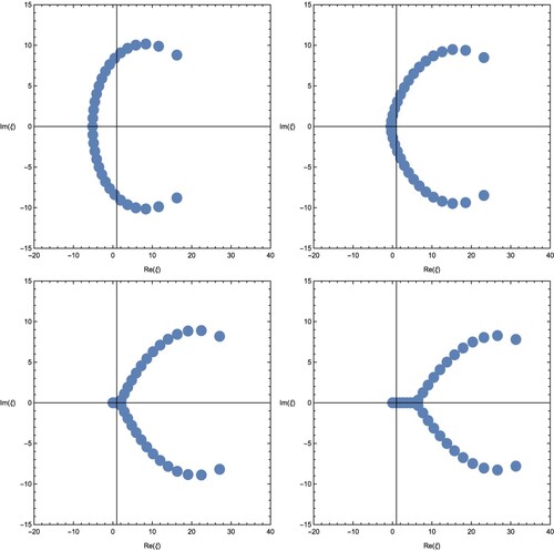
Especially, we take $\lambda =\frac{1}{10}$ (top-left), $\lambda =\frac{5}{10}$ (top-right), $\lambda =\frac{7}{10}$ (bottom-left) and $\lambda =\frac{9}{10}$ (bottom-right) in Figure 1.

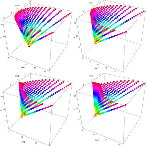
Degenerate FEG polynomials have stacks of zeros for $3\le \omega \le 40$ and u = 2r = 4, forming a 3D structure, as follows (Figure 2): Particularly, we take $\lambda =\frac{1}{10}$ (top-left), $\lambda =\frac{5}{10}$ (top-right), $\lambda =\frac{7}{10}$ (bottom-left) and $\lambda =\frac{9}{10}$ (bottom-right) in Figure 2.

Figure 2. Zeros of ${\mathbb{A}}_{\omega ,\lambda }^{\left(2\right)}(\xi ;u)=0$.

Our next step is to calculate an approximate solution that meets the degenerate FEG polynomials, ${\mathbb{A}}_{\omega ,\lambda }^{\left(2\right)}(\xi ;u)=0$, for u = 4 and $\lambda =\frac{1}{10}.$ Table 1 provides the results as follows.

Table 1. Approximate solutions of ${\mathbb{A}}_{\omega ,\lambda }^{\left(2\right)}(\xi ;4)=0,\lambda =\frac{1}{10}$.

degree ω	ξ
3	$-0.33333$
4	$-0.28333-0.66479i,-0.28333+0.66479i$
5	$-0.71082,0.00541-1.22243i,0.00541+1.22243i$
6	$-0.75445-0.59160i,-0.75445+0.59160i,$
	$0.3878-1.7158i,0.3878+1.7158i$
7	$-1.0512,-0.63075-1.14062i,-0.63075+1.14062i,$
	$0.8230-2.1626i,0.8230+2.1626i$
8	$-1.13131-0.56548i,-1.13131+0.56548i,-0.4120-1.6548i,$
	$-0.4120+1.6548i,1.2933-2.5734i,1.2933+2.5734i$
9	$-1.3791,-1.0854-1.1059i,-1.0854+1.1059i,-0.1309-2.1398i,$
	$-0.1309+2.1398i,1.7892-2.9555i,1.7892+2.9555i$
10	$-1.4778-0.5514i,-1.4778+0.5514i,-0.9552-1.6232i,$
	$-0.9552+1.6232i,0.1949-2.5997i,0.1949+2.5997i,$
	$2.3048-3.3139i,2.3048+3.3139i$
11	$-1.7012,-1.4761-1.0861i,-1.4761+1.0861i,$
	$-0.7640-2.1197i,-0.7640+2.1197i,0.5544-3.0379i,$
	$0.5544+3.0379i,2.8363-3.6524i,2.8363+3.6524i$

6. Zero values of the degenerate CFEG polynomials

In this section, certain zeros of the degenerate CFEG polynomials and beautifully graphical representations are shown.

We remember the definition of degenerate CFEG polynomials from (53(53) $\frac{(1-\phi )({\log }_{\lambda }(1+\varpi ){)}^l}{(1+\varpi )-\phi }(1+\varpi {)}^{\rho }=\sum _{\psi =0}^{\mathrm{\infty }}C{\mathbb{G}}_{\psi ,\lambda }^{(F,l)}(\rho ;\phi )\frac{{\varpi }^{\psi }}{\psi !}.$(53) ) as follows: $\frac{(1-u)({\log }_{\lambda }(1+\tau ){)}^r}{(1+\tau )-u}(1+\tau {)}^{\xi }=\sum _{\omega =0}^{\mathrm{\infty }}C{\mathbb{G}}_{\omega ,\lambda }^{(F,r)}(\xi ;u)\frac{{\tau }^{\omega }}{\omega !}.$We now provide the first few polynomials $C{\mathbb{G}}_{\omega ,\lambda }^{(F,r)}(\xi ;u)$ as follows $\begin{array}{rl}C{\mathbb{G}}_{1,\lambda }^{(F,2)}(\xi ;u)& =0,\\ C{\mathbb{G}}_{2,\lambda }^{(F,2)}(\xi ;u)& =2,\\ C{\mathbb{G}}_{3,\lambda }^{(F,2)}(\xi ;u)& =\frac{12}{-1+u}-\frac{6u}{-1+u}-\frac{6\lambda }{-1+u}+\frac{6u\lambda }{-1+u}-\frac{6\xi }{-1+u}+\frac{6u\xi }{-1+u},\\ C{\mathbb{G}}_{4,\lambda }^{(F,2)}(\xi ;u)& =\frac{24}{(1-u{)}^3}+\frac{22}{(1-u)}+\frac{24}{(-1+u{)}^2}-\frac{24u}{(1-u{)}^3}-\frac{22u}{1-u}-\frac{24u}{(-1+u{)}^2}\\ & -\frac{36\lambda }{1-u}-\frac{24\lambda }{(-1+u{)}^2}+\frac{36u\lambda }{1-u}+\frac{24u\lambda }{(-1+u{)}^2}+\frac{14{\lambda }^2}{1-u}\\ & -\frac{14u\lambda ]2}{1-u}-\frac{36\xi }{1-u}-\frac{24\xi }{(-1+u{)}^2}+\frac{36u\xi }{1-u}+\frac{24u\xi }{(-1+u{)}^2}\\ & +\frac{24\lambda \xi }{1-u}-\frac{24u\lambda \xi }{1-u}+\frac{12{\xi }^2}{1-u}-\frac{12u{\xi }^2}{1-u},\\ C{\mathbb{G}}_{5,\lambda }^{(F,2)}(\xi ;u)& =-\frac{120}{(1-u{)}^3}-\frac{100}{1-u}-\frac{120}{(-1+u{)}^4}-\frac{110}{(-1+u{)}^2}+\frac{120u}{(1-u{)}^3}+\frac{100u}{1-u}\\ & +\frac{120u}{(-1+u{)}^4}+\frac{110u}{(-1+u{)}^2}+\frac{120\lambda }{(1-u{)}^3}+\frac{210\lambda }{1-u}+\frac{180\lambda }{(-1+u{)}^2}\\ & -\frac{120u\lambda }{(1-u{)}^3}-\frac{210u\lambda }{1-u}-\frac{180u\lambda }{(-1+u{)}^2}-\frac{140{\lambda }^2}{1-u}-\frac{70{\lambda }^2}{(-1+u{)}^2}+\frac{140u{\lambda }^2}{1-u}\\ & +\frac{70u{\lambda }^2}{(-1+u{)}^2}+\frac{30{\lambda }^3}{1-u}-\frac{30u{\lambda }^3}{1-u}+\frac{120\xi }{(1-u{)}^3}+\frac{210\xi }{1-u}+\frac{180\xi }{(-1+u{)}^2}\\ & -\frac{120u\xi }{(1-u{)}^3}-\frac{210u\xi }{1-u}-\frac{180u\xi }{(-1+u{)}^2}-\frac{240\lambda \xi }{1-u}-\frac{120\lambda \xi }{(-1+u{)}^2}\\ & +\frac{240u\lambda \xi }{1-u}+\frac{120u\lambda \xi }{(-1+u{)}^2}+\frac{70{\lambda }^2\xi }{1-u}-\frac{70u{\lambda }^2\xi }{1-u}-\frac{120{\xi }^2}{1-u}-\frac{60{\xi }^2}{(-1+u{)}^2}\\ & +\frac{120u{\xi }^2}{1-u}+\frac{60u{\xi }^2}{(-1+u{)}^2}+\frac{(60\lambda {\xi }^2}{1-u}-\frac{60u\lambda {\xi }^2}{1-u}+\frac{20{\xi }^3}{1-u}-\frac{20u{\xi }^3}{1-u}.\end{array}$The zeros of the degenerate CFEG polynomials are plotted for $\omega =33$ and r = 2 (Figure 3):

Figure 3. Zeros of $C{\mathbb{G}}_{\omega ,\lambda }^{(F,r)}(\xi ;u)=0$.

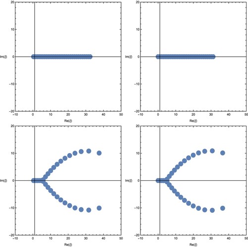
Particularly, we take u = −3 and $\lambda =\frac{1}{10}$ (top-left); u = −3, and $\lambda =\frac{9}{10}$ (top-right); u = 3 and $\lambda =\frac{1}{10}$ (bottom-left) and u = 3 and $\lambda =\frac{9}{10}$ (bottom-right) in Figure 3.

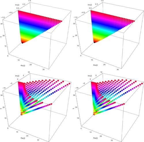
Stacks of zeros of the degenerate CFEG polynomials $C{\mathbb{G}}_{\omega ,\lambda }^{(F,r)}(\xi ;u)$ for $3\le \omega \le 33$, forming a 3D structure, are represented by Figure 4: Specifically, we take u = −3 and $\lambda =\frac{1}{10}$ (top-left); u = −3, and $\lambda =\frac{9}{10}$ (top-right); u = 3 and $\lambda =\frac{1}{10}$ (bottom-left) and u = 3 and $\lambda =\frac{9}{10}$ (bottom-right) in Figure 4.

Figure 4. Zeros of $C{\mathbb{G}}_{\omega ,\lambda }^{(F,r)}(\xi ;u)=0$.

In the next step, we compute an approximate solution that meets the degenerate CFEG polynomials, namely $C{\mathbb{G}}_{\omega ,\lambda }^{(F,r)}(\xi ;u)=0$. Table 2 contains the results as follows.

Table 2. Approximate solutions of $C{\mathbb{G}}_{\omega ,\frac{1}{10}}^{(F,2)}(\xi ;3)=0$.

degree ω	ξ
3	$0.40000$
4	$0.90000-0.57879i,0.90000+0.57879i$
5	$0.47195,1.8640-1.1836i,1.8640+1.1836i$
6	$0.89016-0.19846i,0.89016+0.19846i,2.9098-1.7350i,$
	$2.9098+1.7350i$
7	$0.50506,1.7312-0.8228i,1.7312+0.8228i,$
	$4.0162-2.2423i,4.0162+2.2423i$
8	$0.60428,1.2650,2.6016-1.3597i,2.6016+1.3597i,$
	$5.1638-2.7132i,5.1638+2.7132i$
9	$0.50384,1.7707-0.5556i,1.7707+0.5556i,3.5360-1.8831i,$
	$3.5360+1.8831i,6.3414-3.1542i,6.3414+3.1542i$
10	$0.52280,1.4247,2.5641-1.0649i,2.5641+1.0649i,$
	$4.5199-2.3878i,4.5199+2.3878i,7.5423-3.5701i,7.5423+3.5701i$
11	$0.48645,1.8480-0.2986i,1.8480+0.2986i,3.4047-1.5757i,$
	$3.4047+1.5757i,5.5423-2.8741i,5.5423+2.8741i,$
	$8.7618-3.9647i,8.7618+3.9647i$

7. Conclusion

The pioneer of the degenerate idea was L. Carlitz [4], utilizing the degenerate exponential function which can be interpreted without the limit case of the familiar exponential function. After that, the degenerate logarithm function may be interpreted without the limit case of the usual logarithm function, see [13,26]. By these functions, degenerate forms of many functions, numbers, and polynomials are considered and investigated [1,4–6,8–10,12–14,16,17,21,23–27]. With these ideas and motivation, in this study, we have introduced the degenerate Frobenius-Euler-Genocchi polynomials by using the degenerate exponential function and degenerate Changhee-Frobenius-Euler-Genocchi polynomials by using the degenerate logarithm function. Then, we examined some summation formulas and several correlations with degenerate Stirling numbers of both kinds and degenerate Frobenius-Euler polynomials. Lastly, we have shown certain zeros of both the degenerate FEG polynomials and the degenerate CFEG polynomials and provided their beautifully graphical representations.

Disclosure statement

No potential conflict of interest was reported by the authors.

References

- Alam N, Khan WA, Kızılateş C, et al. Some explicit properties of Frobenius–Euler–Genocchi polynomials with applications in computer modeling. Symmetry. 2023;15(7):1358. doi: 10.3390/sym15071358
- Avazzadeh Z, Hassani H, Agarwal P, et al. Optimal study on fractional fascioliasis disease model based on generalized Fibonacci polynomials. Math Methods Appl Sci. 2023;46(8):9332–9350. doi: 10.1002/mma.v46.8
- Belbachir H, Hadj-Brahim S, Rachidi M. On another approach for a family of Appell polynomials. Filomat. 2018;32(12):4155–4164. doi: 10.2298/FIL1812155B
- Carlitz L. Degenerate Stirling, Bernoulli and Eulerian numbers. Util Math. 1979;15:51–88.
- Duran U, Acikgoz M. On generalized degenerate Gould-Hopper-based fully degenerate Bell polynomials. J Math Comput Sci. 2020;21(3):243–257. doi: 10.22436/jmcs
- Jang LC, Lee JG, Rim SH, et al. On the degenerate Frobenius-Genocchi polynomials. Global J Pure Appl Math. 2015;11(5):3601–3613.
- Khan WA, Nisar KS, Duran U, et al. Multifarious implicit summation formulae of Hermite-based poly-Daehee polynomials. Appl Math Inf Sci. 2018;12(2):305–310. doi: 10.18576/amis/120204
- Khan WA, Muhiuddin G, Muhyi A, et al. Analytical properties of type 2 degenerate poly-Bernoulli polynomials associated with their applications. Adv Differ Equ. 2021;2021:420. doi: 10.1186/s13662-021-03575-7
- Kim T, Kim DS, Kim H-Y, et al. Some results on degenerate Daehee and Bernoulli numbers and polynomials. Adv Differ Equ. 2020;2020:311. doi: 10.1186/s13662-020-02778-8
- Muhiuddin G, Khan WA, Muhyi A, et al. Some results on type 2 degenerate poly-Fubini polynomials and numbers. Comput Modell Eng Sci. 2021;129(2):1051–1073.
- Shams M, Kausar N, Agarwal P, et al. On family of the Caputo-type fractional numerical scheme for solving polynomial equations. Appl Math Sci Eng. 2023;31(1):Article ID 2181959. doi: 10.1080/27690911.2023.2181959
- Alatawi MS, Khan WA. New type of degenerate Changhee-Genocchi polynomials. Axioms. 2022;11:355. doi: 10.3390/axioms11080355
- Khan WA, Ali R, Alzobydi KAH, et al. A new family of degenerate poly-Genocchi polynomials with its certain properties. J Funct Spaces. 2021;2021:Article ID 6660517.
- Khan WA, Alatawi MS. Analytical properties of degenerate Genocchi polynomials the second kind and some of their applications. Symmetry. 2022;14(8):1500. doi: 10.3390/sym14081500
- Kim BM, Jeong J, Rim SH. Some explicit identities on Changhee-Genocchi polynomials and numbers. Adv Differ Equ. 2016;2016:202. doi: 10.1186/s13662-016-0925-0
- Kim T, Kim DS, Kim HK. On generalized degenerate Euler–Genocchi polynomials. Appl Math Sci Eng. 2023;31(1):Article ID 2159958. doi: 10.1080/27690911.2022.2159958
- Lim D. Some identities of degenerate Genocchi polynomials. Bull Korean Math Soc. 2016;53(2):569–579. doi: 10.4134/BKMS.2016.53.2.569
- Belbachir H, Hadj-Brahim S. Some explicit formulas of Euler-Genocchi polynomials. Integers. 2019;19:A28.
- Goubi M. On a generalized family of Euler-Genocchi polynomials. Integers. 2021;21:A48.
- Iqbal A, Khan WA. A new family of generalized Euler-Genocchi polynomials associated with hermite polynomials. In: Kumar R, Verma AK, Sharma TK, Verma OP, Sharma S, editors. Soft computing: theories and applications. Singapore: Springer; 2023. (Lecture notes in networks and systems; vol 627).
- Kim BM, Jang L-.C, Kim W, et al. Degenerate Changhee-Genocchi numbers and polynomials. J Inequal Appl. 2017;2017:294. doi: 10.1186/s13660-017-1572-z
- Iqbal A, Khan WA, Nadeem M. New type of degenerate Changhee–Genocchi polynomials of the second kind. In: Kumar R, Verma AK, Sharma TK, Verma OP, Sharma S, editors. Soft computing: theories and applications. Singapore: Springer; 2023. (Lecture notes in networks and systems; vol. 627).
- Khan WA, Alatawi MS. A note on modified degenerate Changhee-Genocchi polynomials of the second kind. Symmetry. 2023;15(1):136. doi: 10.3390/sym15010136
- Kim T, Kwon HI, Seo JJ. On the degenerate Frobenius-Euler numbers. Global J Pure Appl Math. 2015;11(4):2077–2084.
- Muhiuddin G, Khan WA, Al-Kadi D. Construction on the degenerate poly-Frobenius-Euler polynomials of complex variable. J Funct Spaces. 2021;2021:Article ID 3115424. doi: 10.1155/2021/3115424
- Kim T. A note on degenerate Stirling numbers of the second kind. Proc Jangjeon Math Soc. 2018;21(4):58–598.
- Khan WA, Muhyi A, Ali R, et al. A new family of degenerate poly-Bernoulli polynomials of the second kind with its certain related properties. AIMS Math. 2021;6(11):12680–12697. doi: 10.3934/math.2021731
- Khan WA, Haroon H. Some symmetric identities for the generalized Bernoulli, Euler and Genocchi polynomials associated with Hermite polynomials. Springer Plus. 2016;5:1920. doi: 10.1186/s40064-016-3585-3