Triangular intuitionistic fuzzy linear system of equations with applications: an analytical approach

Abstract

This study extended an existing semi-analytical technique, the Homotopy Perturbation Method, to the Block Homotopy Modified Perturbation Method by solving two $n\times n$ crisp triangular intuitionistic fuzzy (TIF) systems of linear equations. In the original system, the coefficient matrix is considered as real crisp, while the unknown variable vector and right hand side vector are regarded as triangular intuitionistic fuzzy numbers. The Block Homotopy Modified Perturbation Method is found to be efficient and practical to solve $n\times n$ TIF linear systems as it only requires the non-singularity of the $n\times n$ TIF linear system's coefficient matrix, whereas the point Homotopy Perturbation Method and other classical numerical iterative methods typically require non-zero diagonal entries in the coefficient matrix. A set of theorems relevant to this study are presented and demonstrated. We solve an engineering application, i.e. a current flow circuit problem that is represented in terms of a triangular intuitionistic fuzzy environment, using the suggested method. The unknown current is then obtained as a triangle intuitionistic fuzzy number. The proposed semi-analytic method is used to solve some numerical test problems in order to validate their performance and efficiency in comparison to other existing techniques. The numerical results of the example are displayed on graphs with different degrees of uncertainty. The efficiency and accuracy of the proposed method are further demonstrated by comparisons to block Jacobi, Adomain Decomposition method, Successive Over-Relaxation method and the classical Gauss-Seidel numerical method.

KEYWORDS:

• Triangular intuitionistic fuzzy linear system
• semi analytical method
• iterative methods
• computational CPU-time
• triangular intuitionistic fuzzy solution

SUBJECT CLASSIFICATION CODE:

• 08A72
• 34A34
• 65F05
• 65F10
• 65F99

1. Introduction

Systems of linear equations are used in many areas of chemical, biological, mathematical, physical, and engineering sciences, such as transportation system, circuit analysis, heat transport, structural and analytical mechanics, heat and mass transfer, fluid flow, and among others (see e.g. [1–5]). Most problems we solve involve working with imprecise data. We can avoid these errors by representing the given data as fuzzy and more generally intuitionistic fuzzy numbers. Fuzzy set theory was first proposed by Zadeh [6]. The arithmetic operations with fuzzy numbers were first introduced and analysed in [7–13]. Fuzzy system of nonlinear equations play a significant role in modelling physical and engineering problems due to their ability to simulate real situation in order to deal with ambiguous systems. A fuzzy linear system of equations is a useful tool that accommodates fuzziness and uncertainty in situations like these. When there are linear relationships among variables that are interpreted in triangle intuitionistic fuzzy form, a triangular intuitionistic fuzzy system of equations must be used for the problem's linear optimization. Triangular intuitionistic fuzzy linear systems of equations are very beneficial for measuring unknown current in sophisticated pattern while analyzing circuits.

However, exact solutions to large fuzzy systems of linear equations (FSLEs) are difficult to achieve because of the complexity of the exact techniques required to obtain the exact solution. As a result, handling the corresponding FSLEs may necessitate the use of reliable and efficient numerical techniques. Therefore, in most of real world problems, the system parameters are expressed as triangular fuzzy numbers. Fuzzy linear systems of equations have been the subject of several studies, many of which discuss their practical applications. The present analysis makes use of the findings from several of these studies. Friedman et al. [14] presented a general method for solving a $n\times n$ fuzzy linear system with a crisp coefficient matrix and an arbitrary fuzzy number vector in the right hand column. The authors replaced the original $n\times n$ fuzzy linear system with a crisp $2n\times 2n$ linear system using the embedding method described in [15]. Solving a fuzzy linear system is therefore identical to solving a crisp linear system. Traditional point iterative techniques, like Jacobi, Gauss-Seidel, SOR and conjugate gradient methods fail when a diagonal element of the coefficient matrix is zero. As a result, analytical or semi-analytical approaches are used to solve a fuzzy linear system of equations.

Numerous methods have been used in recent years to solve fuzzy linear systems of equations with various fuzzy numbers, including the iterative algorithm [14], Conjugate Gradient Method [15], exact methods [16–18], Steepest Descent Method [19], Optimization Method [20], Grobner Bases [21], and LU Decomposition Method [22,23]. To solve triangular fuzzy linear system of equations, Buckly et al. [24] used a-cut method and triangular fuzzy number [25], Allahviranloo et al. [26] used Newton's method. Cho et al. [27] solved fuzzy linear systems of equations in probabilistic norm spaces, while Dennis et al. [28] used Numerical Methods for Unconstrained Optimization and fuzzy nonlinear systems of Equations. Sulaiman et al. [29] used Levenberg-Marquardt method to solve fuzzy nonlinear equations, Ma et al. [30] discussed fuzzy dynamic systems, Mosleh [31] found the solution of dual fuzzy polynomial equations by modified Adomian decomposition method [32,33], Akram et al. [34–37] solved bipolar fuzzy linear system of equations. Jafari et al. [38–41] solved fuzzy linear system of equation using Fuzzy control system. He et al. [42] developed the homotopy perturbation method, an analytic method for nonlinear problems based on basic homotopy principles. The Homotopy Perturbation Method (HPM) combines classical perturbation with homotopy in topology to transform the original problem into a simple, fundamental one [43,44]. Najafi et al. [45–48] used homotopy perturbation method and its application in linear programming problems [49]. Using HPM frequently results in a relatively quick convergence of the solution series, with only a few iterations producing very precise outcomes. The HPM was utilized to solve fuzzy linear systems using triangular fuzzy numbers in [50–53], and [54], but we used the most generalized fuzzy number, TIF number [55–58]. According to exact, analytical, semi-analytical, and numerical approaches, Table 1 analyses recent research contributions for the solving linear system of equations using a variety of fuzzy numbers.

Table 1. Compares recent research contributions for the solving linear system of equations using fuzzy numbers based on exact, analytical, semi-analytical, and numerical technique.

Authors	Year	Fuzzy number	Scheme
Amit et al. [59]	2011	Triangular fuzzy number	AT
Allahviranloo et al. [60]	2011	Arbitrary fuzzy number	SAT
Ezzati et al. [61]	2012	LR-Type fuzzy numebr	NT
Behera et al. [62]	2013	Complex fuzzy number	ET
Lodwick et al. [63]	2015	Interval type fuzzy number	ET
Akram et al. [64]	2019	m-bipolar fuzzy number	NT
Mikaeilvand et al. [65]	2020	Arbitrary fuzzy number	ET
Saqib et al. [66]	2020	bipolar fuzzy number	NT
Akram et al. [67]	2020	LR-bipolar fuzzy number	NT
Akram et al. [68]	2021	Bipolar fuzzy number	NT

where ET stands for Exact, AT for analytical, SAT for semi-analytical and NT for numerical technique for solving fuzzy linear system of equations.

1.1. Motivation

Our analysis of the literature shows that the number of works on intuitionistic systems of linear equations that employ exact and numerical techniques is somewhat limited. However, almost no research has been done on utilizing analytical techniques to solve intuitionistic fuzzy systems of linear equations. Consequently, working in this area has a lot of potential and opportunity. Since there hasn't been much research on solving fuzzy systems of linear equations, new, efficient analytical techniques must be developed. Motivated by the studies mentioned above, the main goal of the present work is to develop and analyse the Block Homotopy Modified Perturbation Method (BHMPM) for solving $n\times n$ fuzzy linear systems. The BHMPM is efficient and practical as it only requires the non-singularity of the $n\times n$ fuzzy linear systems coefficient matrix, whereas the point HPM method usually requires nonzero diagonal entries in the coefficient matrix. This article may be useful to other researchers in the future as they work to improve the analytical methods used to solve fuzzy systems of linear equations using broader definitions of fuzzy numbers.

1.2. Novelty

An innovative and efficient analytical approach is presented in this article for solving TIFLSEs, which is a significant contribution to the area, and gives a comprehensive approach to TIFLSEs models, which are applicable to real-world problems. These responses provide a more in-depth understanding of TIFLSEs and their importance in a variety of scientific and technical disciplines. To demonstrate the practical use of the suggested technique, the paper solves an electrical circuit problem. These examples demonstrate how successful and practical the proposed strategy is for resolving real-world problems. To solve TIFLSEs problems, these methods are inventive and provide a novel approach.

To illustrate the validity of the proposed techniques, some numerical test problems are considered. The main objective of this research work are summarized below.

• BHMPM is developed and analysed to solve systems of TIF equations.

• The computing complexity of the proposed BHMPM is examined in order to solve an unexplored linear system of TIF equations.

• Numerical examples of a linear system of equations are taken into consideration in a TIF environment.

• Use a triangular intuitionistic fuzzy system of linear equations (TIFLSEs) to solve a problem in engineering.

• The efficiency and viability of the proposed approach are assessed using computational techniques.

• The graphical solutions of the triangular linear intuitionistic fuzzy system of linear equations are analysed and discussed.

This article is divided into five sections. We look at some basic definitions and arithmetic operations of triangular, trapezoidal and intuitionistic fuzzy number in Section 2. We propose and analyse BHMPM iterative method for solving TIF linear system of equations (TIFLSEs) in Section 3. In Section 4, we demonstrate various numerical test examples and make conclusions in the last section.

2. Preliminaries

According to [6–10], the basic concept of a fuzzy set is as follows:

Definition 2.1:

If H₁, is a collection of objects and its objects are denoted by x then fuzzy ser H in H₁, is a set of order pairs $H=\left\{x,{\xi }_{{\tilde{a}}_1}\left(x\right):x\in H_1\right\}$where ${\xi }_{{\tilde{a}}_1}\left(x\right)=H_1\to [0,1]$ is define the membership function. In order pair $\left(x,{\xi }_{{\tilde{a}}_1}\left(x\right)\right),$ $x\in H_1$ and ${\xi }_{{\tilde{a}}_1}\left(x\right)\in [0,1].$

Definition 2.2:

A fuzzy number is a fuzzy set, similar to $x:R\to I=[0,1]$ which satisfies [13] and [9]:

1. $x\left(r\right)$ is upper semi continuous,

2. $x\left(r\right)=0$ outside some interval $[e_1,e_2]$,

3. there are real numbers $a_1,a_2$ such that $e_1\le a_1\le a_2\le e_2$ and

   1. $x\left(r\right)$ is monotonic increasing on $[e_1,a_1]$

   2. $x\left(r\right)$ is monotonic decreasing on $[a_2,e_2]$

   3. $x\left(r\right)=1$, for $[a_1\le r\le a_2]$

In parametric form, a fuzzy number is defined as:

Definition 2.3:

We denote by E, the set of all fuzzy numbers. An equivalent parametric form is also given in [69] and [70] as follows:

1. $x^L\left(r\right)$ is a bounded monotonic increasing left continuous function,

2. $x^U\left(r\right)$ is a bounded monotonic decreasing left continuous function,

3. $x^L\left(r\right)\le x^U\left(r\right),$ $0\le r\le 1.$

The definitions for triangular and trapezoidal fuzzy numbers are as follows:

Definition 2.4:

A popular fuzzy number is the trapezoidal fuzzy [32] number $A,$ denoted by $A=\left({\ddot{e}}_1,{\ddot{e}}_2,{\ddot{e}}_3,{\ddot{e}}_4;\text{ß}\right),0<$ ß $<1,$ is a fuzzy number with membership function as: $\xi \left(x\right)=\{\begin{array}{ll}{\displaystyle \frac{x-{\ddot{e}}_1}{{\ddot{e}}_2-{\ddot{e}}_1}}& \text{if }{\ddot{e}}_1<x<{\ddot{e}}_2,\\ 1& \text{if }x\in [{\ddot{e}}_2,{\ddot{e}}_3],\\ {\displaystyle \frac{{\ddot{e}}_4-x}{{\ddot{e}}_4-{\ddot{e}}_3}}& {\ddot{e}}_3<x<{\ddot{e}}_4,\\ 0& \text{otherwise}.\end{array}$and its parametric from $x^L\left(r\right)={\ddot{e}}_1+r({\ddot{e}}_2-{\ddot{e}}_1);x^U\left(r\right)={\ddot{e}}_4-r({\ddot{e}}_4-{\ddot{e}}_3).$

Definition 2.5:

If ${\ddot{e}}_2={\ddot{e}}_3,$ then $A\left(x\right)=\left({\ddot{e}}_1/{\ddot{e}}_2/{\ddot{e}}_4\right)$ is known as triangular fuzzy number [75]. An intuitionistic fuzzy set, which is a generalization of fuzzy set, is defined as follows:

Definition 2.6:

Assume for fixed set $X$ an intuitionistic fuzzy set [71] $H$ in $X$ is $H=\left\{〈x,{\xi }_{{\tilde{a}}_1}\left(x\right){\xi }_{{\tilde{a}}_2}\left(x\right)〉0:x\in X\right\},$where ${\xi }_{{\tilde{a}}_1}\left(x\right):X\to [0,1],{\xi }_{{\tilde{a}}_2}\left(x\right):X\to [0,1]$define the membership and non-membership function respectively and $x\in X,0<{\xi }_{{\tilde{a}}_1}\left(x\right){\xi }_{{\tilde{a}}_2}\left(x\right)\le 1.$

Definition 2.7:

An intuitionistic fuzzy set [72] $H=\left\{x,{\xi }_{{\tilde{a}}_1}\left(x\right),{\xi }_{{\tilde{a}}_2}\left(x\right)\mathrm{\setminus }x\in X\right\}$such that ${\xi }_{{\tilde{a}}_1}\left(x\right)$ and $1-{\xi }_{{\tilde{a}}_1}\left(x\right),\mathrm{\forall x}\in R$ are fuzzy numbers called intuitionistic fuzzy numbers.

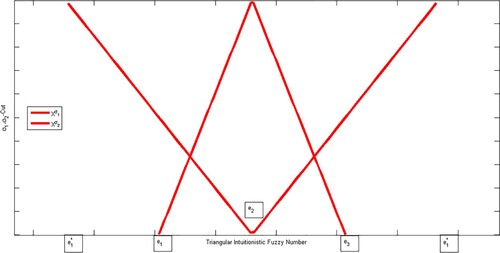
Definition 2.8:

A triangular intuitionistic fuzzy number (TIFN) (see [73]) $H_1$ is a subset of TIFN having the following membership ${\xi }_{{\ddot{e}}_m}^{\ast }\left(x\right)=\{\begin{array}{ll}{\displaystyle \frac{x-{\ddot{e}}_1}{{}_{{\ddot{e}}_2}{-}_{{\ddot{e}}_1}}}& \text{for }{\ddot{e}}_1\le x<{\ddot{e}}_2,\\ {\displaystyle \frac{x-{\ddot{e}}_3}{{}_{{\ddot{e}}_2}{-}_{{\ddot{e}}_3}}}& \text{for }{\ddot{e}}_2<x\le {\ddot{e}}_3,\\ 0& \text{otherwise,}\end{array}$non-membership function ${\xi }_{{\ddot{e}}_n}\left(x\right)=\{\begin{array}{ll}{\displaystyle \frac{{\ddot{e}}_2-x}{{}_{{\ddot{e}}_2}{-}_{{\ddot{e}}_1^{\ast }}}}& \text{for }{\ddot{e}}_1^{\ast }\le x<{\ddot{e}}_2,\\ {\displaystyle \frac{x-{\ddot{e}}_2}{{}_{{\ddot{e}}_3^{\ast }}{-}_{{\ddot{e}}_2}}}& \text{for }{\ddot{e}}_2<x\le {\ddot{e}}_3^{\ast },\\ 0& \text{otherwise}\end{array}$and its parametric form is $\begin{array}{rl}[{\ddot{e}}_n{]}_{({\sigma }_1,{\sigma }_2)}& =[{\ddot{e}}_1+r({\ddot{e}}_2-{\ddot{e}}_1),{\ddot{e}}_3-r({\ddot{e}}_3-{\ddot{e}}_2);{\ddot{e}}_2\\ & -r({\ddot{e}}_2-{\ddot{e}}_1^{\ast }),{\ddot{e}}_2+r({\ddot{e}}_3^{\ast }-{\ddot{e}}_2)],\end{array}$where ${\ddot{e}}_1^{\ast }\le {\ddot{e}}_2\le {\ddot{e}}_3^{\ast }$; ${\ddot{e}}_1\le {\ddot{e}}_2\le {\ddot{e}}_3.$ Triangular intuitionistic fuzzy number is geometrically presented in Figure 1.

Figure 1. Shows triangular intuitionistic fuzzy number.

Definition 2.9:

$A=〈\left({\ddot{e}}_1^{\ast },{\ddot{e}}_1,{\ddot{e}}_2,{\ddot{e}}_3,{\ddot{e}}_3^{\ast }\right)〉$ and $B=〈{\stackrel{⌣}{a}}_1^{\ast },{\stackrel{⌣}{a}}_1,{\stackrel{⌣}{a}}_2,{\stackrel{⌣}{a}}_3,{\stackrel{⌣}{a}}_3^{\ast }〉$ are said to be equal iff $A=B$ $i.e.,$ $〈{\ddot{e}}_1^{\ast }={\stackrel{⌣}{a}}_1^{\ast },{\ddot{e}}_1={\stackrel{⌣}{a}}_1,{\ddot{e}}_2={\stackrel{⌣}{a}}_2,{\ddot{e}}_3={\stackrel{⌣}{a}}_3,{\ddot{e}}_3^{\ast }={\stackrel{⌣}{a}}_3^{\ast }〉$, $A\oplus B=〈{\ddot{e}}_1^{\ast }+{\stackrel{⌣}{a}}_1^{\ast },{\ddot{e}}_1+{\stackrel{⌣}{a}}_1,{\ddot{e}}_2+{\stackrel{⌣}{a}}_2,{\ddot{e}}_3+{\stackrel{⌣}{a}}_3,{\ddot{e}}_3^{\ast }+{\stackrel{⌣}{a}}_3^{\ast }〉,$ $A\otimes B=〈{\ddot{e}}_1^{\ast }\ast {\stackrel{⌣}{a}}_1^{\ast },{\ddot{e}}_1\ast {\stackrel{⌣}{a}}_1,{\ddot{e}}_2\ast {\stackrel{⌣}{a}}_2,{\ddot{e}}_3\ast {\stackrel{⌣}{a}}_3,{\ddot{e}}_3^{\ast }\ast {\stackrel{⌣}{a}}_3^{\ast },{\ddot{e}}_i,{\stackrel{⌣}{a}}_i\ge 0,i=1\dots 3〉$ and $\mathrm{kA}=\{\begin{array}{c}〈\left(k{\ddot{e}}_1^{\ast },k{\ddot{e}}_1,k{\ddot{e}}_2,k{\ddot{e}}_3,k{\ddot{e}}_3^{\ast }\right)〉,k>0,\\ 〈\left(k{\ddot{e}}_3^{\ast },k{\ddot{e}}_3,k{\ddot{e}}_2,k{\ddot{e}}_1,k{\ddot{e}}_1^{\ast }\right)〉k<0.\end{array}.$For more arithmetic operations see [74].

Definition 2.10:

The $n\times n$ linear systems [75] (1) $\{\begin{array}{c}{\tilde{a}}_{11}{x}_1+{\tilde{a}}_{12}{x}_2+\dots .{\tilde{a}}_{1n}{x}_n=y_1,\\ {\tilde{a}}_{11}{x}_1+{\tilde{a}}_{12}{x}_2+\dots .{\tilde{a}}_{1n}{x}_n=y_2,\\ ⋮\\ {\tilde{a}}_{n1}{x}_1+{\tilde{a}}_{n2}{x}_2+\dots .{\tilde{a}}_{\mathrm{nn}}{x}_n=y_n.\end{array}$(1) or briefly $\mathrm{AX}=Y,$where $A=\left({\tilde{a}}_{\mathrm{ij}}\right)$, $1\le i,t\le n$ is a crisp matrix, $Y=(y_1,y_2,\dots y_n{)}^T$ is known $y_i\mathrm{ϵE}$ and $X=(x_1,x_2,..,x_n{)}^T$ is unknown $x_i\mathrm{ϵE}$, $1\le i\le n,$ is called a TIFLSEs.

Definition 2.11:

A fuzzy number vector $X=(x_1,x_2,\dots x_n{)}^T$ given by $x_t=\left(x_t^{L_1}\right({\sigma }_1),x_t^{U_1}({\sigma }_1),x_t^L({\sigma }_2),x_t^U({\sigma }_2\left)\right)$, $1\le t\le n,$ $0\le {\sigma }_1,{\sigma }_2\le 1$, is called solution of the TIFLSEs (1) if (2) $\{\begin{array}{rl}{\left(\sum _{t=1}^n{\tilde{a}}_{\mathrm{it}}{x}_t\right)}^L& =\sum _{t=1}^n\left[{\tilde{a}}_{\mathrm{it}}^L{x}_t^L\right]=y_i^L,\\ {\left(\sum _{t=1}^n{\tilde{a}}_{\mathrm{it}}{x}_t\right)}^U& =\sum _{t=1}^n\left[{\tilde{a}}_{\mathrm{it}}^U{x}_t^U\right]=y_i^U,\\ {\left(\sum _{t=1}^n{\tilde{a}}_{\mathrm{it}}{x}_t\right)}^L& =\sum _{t=1}^n\left[{\tilde{a}}_{\mathrm{it}}^L{x}_t^L\right]=y_i^L,\\ {\left(\sum _{t=1}^n{\tilde{a}}_{\mathrm{it}}{x}_t\right)}^U& =\sum _{t=1}^n\left[{\tilde{a}}_{\mathrm{it}}^U{x}_t^U\right]=y_i^U.\end{array}i=1,..n$(2) By (2) and the operation of fuzzy numbers, Friedman et al. [73] replace the original TIFLSEs (1) by an $2n\times 2n$ crisp linear system. (3) $\begin{array}{rl}S{X}^{{\xi }_{{\ddot{e}}_m}^{\ast }}& =Y^{{\xi }_{{\ddot{e}}_m}^{\ast }}\text{ or }\left[\begin{array}{cc}{B}_{11}^{\ast }& C_{11}^{\ast }\\ C_{11}^{\ast }& B_{11}^{\ast }\end{array}\right]\left[\begin{array}{c}{X}^{L_1}\\ X^{U_1}\end{array}\right]=\left[\begin{array}{c}{Y}^{L_1}\\ -Y^{U_1}\end{array}\right],\\ S{X}^{{\xi }_{{\ddot{e}}_m}}& =Y^{{\xi }_{{\ddot{e}}_m}}\text{ or }\left[\begin{array}{cc}{B}_{11}^{\ast }& C_{11}^{\ast }\\ C_{11}^{\ast }& B_{11}^{\ast }\end{array}\right]\left[\begin{array}{c}{X}^L\\ X^U\end{array}\right]=\left[\begin{array}{c}{Y}^U\\ -Y^U\end{array}\right],\end{array}$(3) where $S=\left(S_{\mathrm{kl}}\right)$, 1 $\le k,l\le 2n,s_{\mathrm{kl}}$ are determined as follows $\begin{array}{rl}{\tilde{a}}_{\mathrm{it}}& \ge 0\Rightarrow S_{\mathrm{it}}=S_i+m,t+n={\tilde{a}}_{\mathrm{it},}\\ {\tilde{a}}_{\mathrm{it}}& <0\Rightarrow S_{\mathrm{it}},t+n=-{\tilde{a}}_{\mathrm{ij}},S_i+m,t={\tilde{a}}_{\mathrm{it},}\end{array}$and any $S_{\mathrm{kl}}$ which is not determined by the above items is zero and for ${\sigma }_1-\mathrm{Cut}$ $X^{{\xi }_{{\ddot{e}}_m}^{\ast }}=\left[\begin{array}{c}{X}^{L_1}\\ -X^{U_1}\end{array}\right]=\left[\begin{array}{c}{x}_1^{L_1}\\ .\\ .\\ .\\ x_n^{L_1}\\ -x_1^{U_1}\\ .\\ .\\ .\\ -x_n^{U_1}\end{array}\right],$ $Y^{{\xi }_{{\ddot{e}}_m}^{\ast }}=\left[\begin{array}{c}{Y}^{L_1}\\ -Y^{U_1}\end{array}\right]=\left[\begin{array}{c}{y}_1^{L_1}\\ .\\ .\\ .\\ y_n^{L_1}\\ -y_1^{U_1}\\ .\\ .\\ .\\ -y_n^{U_1}\end{array}\right]$and ${\sigma }_2-\text{Cut}$ is $X^{{\xi }_{{\ddot{e}}_m}}=\left[\begin{array}{c}{X}^L\\ -X^U\end{array}\right]=\left[\begin{array}{c}{x}_1^L\\ .\\ .\\ .\\ x_n^L\\ -x_1^U\\ .\\ .\\ .\\ -x_n^U\end{array}\right],$ $Y^{{\xi }_{{\ddot{e}}_m}}=\left[\begin{array}{c}{Y}^L\\ -Y^U\end{array}\right]=\left[\begin{array}{c}{y}_1^L\\ .\\ .\\ .\\ y_n^L\\ -y_1^U\\ .\\ .\\ .\\ -y_n^U\end{array}\right].$The matrix $B_{11}^{\ast }$ has the positive entries for $A,C_{11}^{\ast }$, the absolute of the negative for $A$, and $A=B_{11}^{\ast }-C_{11}^{\ast }$ . It is equivalent to solving the crisp linear system (3) to solve the fuzzy linear system (If and only if the coefficient matrix S is not singular), the crisp linear system (3) can be uniquely solved for X. The following theorem describes when S is non-singular.

Theorem 2.1:

The matrix S is non-singular if and only if $A=B_{11}^{\ast }-C_{11}^{\ast }$ and $B_{11}^{\ast }+C_{11}^{\ast }$ are both non-singular. Matrix $B^{\ast }$ contains the positive entries of $A,C_{11}^{\ast }$, the absolute of the matrix. The solution vector X $X^{{\xi }_{{\ddot{e}}_m}^{\ast }},$ $X^{{\xi }_{{\ddot{e}}_m}}$ represent a solution fuzzy vector to the TIFLSEs (1) if and only if $\left(x_t^{L_1}\left({\sigma }_1\right),x_t^{U_1}\left({\sigma }_1\right),x_t^L\left({\sigma }_2\right),x_t^U\left({\sigma }_2\right)\right)$is a TIF number for all $t$.

Definition 2.12:

[57] Let (4) $X=\left\{x_t^{L_1}\left({\sigma }_1\right),x_t^{U_1}\left({\sigma }_1\right),x_t^L\left({\sigma }_2\right),x_t^U\left({\sigma }_2\right)\right\},1\le t\le n$(4) represent the solution of (3). They have a vector of fuzzy numbers. (5) $E=\left\{\left(E_t^{L_1}\right({\sigma }_1),E_t^{U_1}({\sigma }_1),E_t^L({\sigma }_2),E_t^U({\sigma }_2),1\le t\le n\right\}$(5) defined by (6) $\{\begin{array}{c}{E}_t^{L_1}\left({\sigma }_1\right)=min\left\{x_t^{L_1}\right({\sigma }_1),x_t^{U_1}({\sigma }_1),x_t^L({\sigma }_2),\\ x_t^U\left({\sigma }_2\right),x_t^{L_1}\left(1\right),x_t^{U_1}\left(1\right),x_t^L\left(1\right),x_t^U\left(1\right)\}\\ E_t^{U_1}\left({\sigma }_1\right)=max\left\{x_t^{L_1}\right({\sigma }_1),x_t^{U_1}({\sigma }_1),x_t^L({\sigma }_2),\\ x_t^U\left({\sigma }_2\right),x_t^{L_1}\left(1\right),x_t^{U_1}\left(1\right),x_t^L\left(1\right),x_t^U\left(1\right)\}\\ E_t^L\left({\sigma }_2\right)=min\left\{x_t^{L_1}\right({\sigma }_1),x_t^{U_1}({\sigma }_1),x_t^L({\sigma }_2),\\ x_t^U\left({\sigma }_2\right),x_t^{L_1}\left(1\right),x_t^{U_1}\left(1\right),x_t^L\left(1\right),x_t^U\left(1\right)\}\\ E_t^U\left({\sigma }_2\right)=max\left\{x_t^{L_1}\right({\sigma }_1),x_t^{U_1}({\sigma }_1),x_t^L({\sigma }_2),\\ x_t^U\left({\sigma }_2\right),x_t^{L_1}\left(1\right),x_t^{U_1}\left(1\right),x_t^L\left(1\right),x_t^U\left(1\right)\}\end{array}$(6) is called the fuzzy solution of (3). If $\left(x_t^{L_1}\left({\sigma }_1\right),x_t^{U_1}\left({\sigma }_1\right),x_t^L\left({\sigma }_2\right),x_t^U\left({\sigma }_2\right)\right)$, $1\le t\le n$ are all TIF number then (7) $\left(\begin{array}{c}{E}_t^{L_1}\left({\sigma }_1\right)=x_t^{L_1}\left({\sigma }_1\right),E_t^{U_1}\left({\sigma }_1\right)=x_t^{U_1}\left({\sigma }_1\right),\\ E_t^L\left({\sigma }_1\right)=x_t^L\left({\sigma }_1\right),E_t^U\left({\sigma }_1\right)=x_t^U\left({\sigma }_1\right)\end{array}\right),1\le t\le n$(7) and E is called a strong TIF solution. Otherwise, E is called a weak TIF number solution [76,77].

The following theorem [78] gives the unique solution of TIF linear system of equations.

Theorem 2.2:

Let $S$ be non-singular. Then the unique solution $X$ of (3) is always a fuzzy vector for arbitrary vector $Y$, if $S^{-1}$ is non-negative.

Proof:

It is sufficient to show that definition is hold for X. It is clear that have the same structure like S, i.e. (8) $S^{-1}=\left[\begin{array}{cc}{B}_{11}^{\ast }& C_{11}^{\ast }\\ C_{11}^{\ast }& B_{11}^{\ast }\end{array}\right],$(8) from $X=S^{-1}Y,$ we have for ${\sigma }_1-\text{Cut}$ (9) $\{\begin{array}{c}{B}_{11}^{\ast }{Y}^{L_1}-C_{11}^{\ast }{Y}^{U_1}=X^{L_1},\\ -C_{11}^{\ast }{Y}^{L_1}+B_{11}^{\ast }{Y}^{U_1}=X^{U_1},\end{array}$(9) and for ${\sigma }_2-\text{Cut}$ (10) $\{\begin{array}{c}{B}_{11}^{\ast }{Y}^L-C_{11}^{\ast }{Y}^U=X^L,\\ -C_{11}^{\ast }{Y}^L+B_{11}^{\ast }{Y}^U=X^U.\end{array}$(10) Thus (11) $(X^{U_1}-X^{L_1})=\left(B_{11}^{\ast }+C_{11}^{\ast }\right)\left(Y^{U_1}-Y^{L_1}\right)\ge 0$(11) and (12) $(X^U-X^L)=\left(B_{11}^{\ast }+C_{11}^{\ast }\right)\left(Y^U-Y^L\right)\ge 0,$(12) because $(S^{-1}{)}_{\mathrm{ij}}\ge 0$ and $\left(Y^{U_1}-Y^{L_1}\right)\ge 0,\left(Y^U-Y^L\right)\ge 0.$ As $Y=\left[Y^{{\xi }_{{\ddot{e}}_m}^{\ast }},Y^{{\xi }_{{\ddot{e}}_m}}\right]=\left(\left[Y^{L_1},Y^{U_1}\right],\left[Y^L,Y^U\right]\right).$ Since $Y^{U_1},Y^U$ are monotonically decreasing and $Y^{L_1},Y^L$ are monotonically increasing, (9) is also necessary and sufficient for $X^{U_1},X^U$ are monotonically decreasing and $X^{L_1},X^L$ are monotonically increasing, respectively. The bounded left continuity of $X^{U_1},X^U$ is obvious since they are the linear combination of $Y^{U_1},Y^U.$ Hence the theorem is proved.

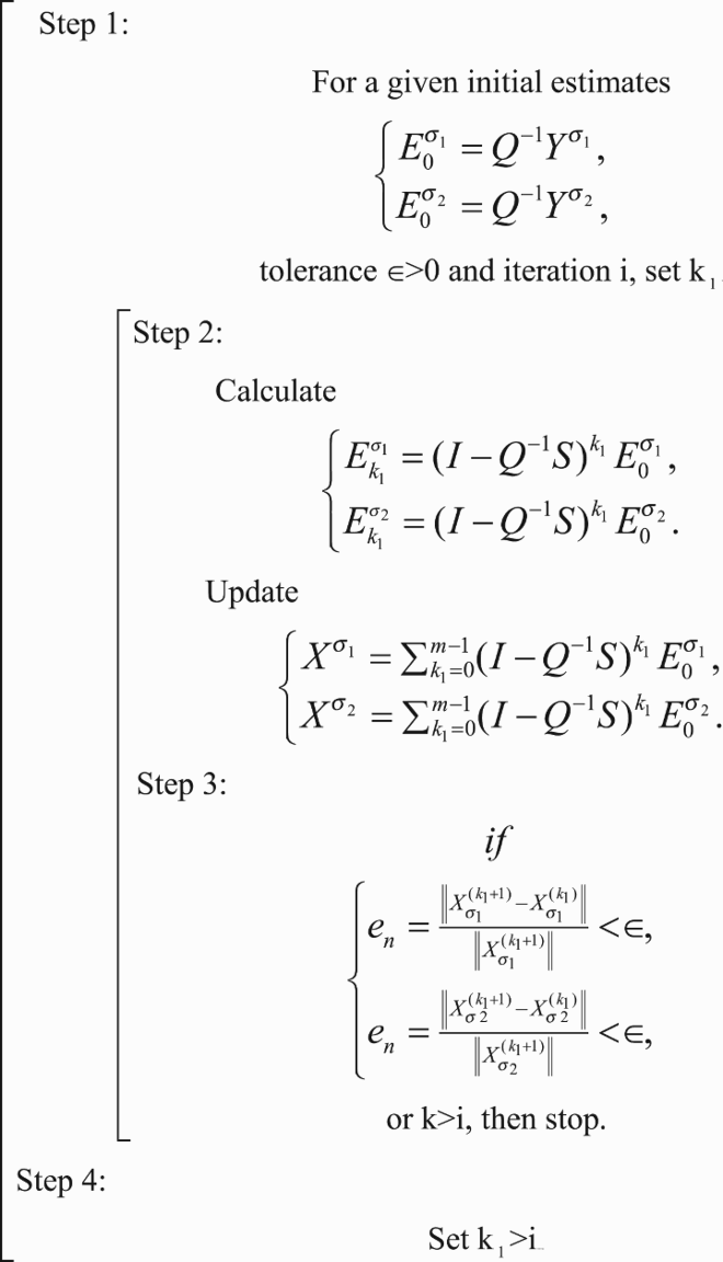
3. Block homotopy modified perturbation method (BHMPM)

The block HPM is an effective and practical approach for solving $n\times n$ triangular intuitionistic fuzzy linear systems, as it only requires the non-singularity of the $n\times n$ triangular coefficient matrix, whereas other methods such as the point HPM method and classical numerical iterative methods typically require non-zero diagonal entries in the coefficient matrix. Therefore, the BHMPM is a useful tool for solving TIFLSEs. Consider (13) $\{\begin{array}{c}L\left(E^{{\sigma }_1}\right)=S{E}^{{\sigma }_1}-Y,F\left(E^{{\sigma }_1}\right)=Q{E}^{{\sigma }_1}-Y,\\ L\left(E^{{\sigma }_2}\right)=S{E}^{{\sigma }_2}-Y,F\left(E^{{\sigma }_2}\right)=Q{E}^{{\sigma }_2}-Y,\end{array}$(13) where $Q$ is nonsingular. We homotopy $H(E,p)$ by (14) $\{\begin{array}{c}H(E^{{\sigma }_1},O)=F\left(E^{{\sigma }_1}\right),H(E^{{\sigma }_1},1)=L\left(E^{{\sigma }_1}\right),\\ H(E^{{\sigma }_2},O)=F\left(E^{{\sigma }_2}\right),H(E^{{\sigma }_2},1)=L\left(E^{{\sigma }_2}\right).\end{array}$(14) By choosing a convex homotopy as: (15) $\{\begin{array}{c}H(E^{{\sigma }_1},p)=(1-p)F\left(E^{{\sigma }_1}\right)+pL\left(E^{{\sigma }_1}\right)=0,\\ H(E^{{\sigma }_2},p)=(1-p)F\left(E^{{\sigma }_2}\right)+pL\left(E^{{\sigma }_2}\right)=0\end{array}$(15) and continuously trace an implicitly curve from a starting point  $H(E^{{\sigma }_1},0),$ $H(E^{{\sigma }_2},0)$ to a solution  $H(E^{{\sigma }_1},1),$ $H(E^{{\sigma }_2},1)$ . The embedding parameter  $p$ monotonically increases from zero to one as the trivial problem  $F\left(E^{{\sigma }_1}\right)=0,$ $F\left(E^{{\sigma }_2}\right)=0$ are continuously the original problem  $L\left(E^{{\sigma }_1}\right)=0,$ $L\left(E^{{\sigma }_2}\right)=0$ . The embedding parameter $p$ belong to $[0,1]$ can be considered as an expanding parameter [14] as: (16) $\{\begin{array}{c}{E}^{{\sigma }_1}=E_0^{{\sigma }_1}+p{E}_1^{{\sigma }_1}+p^2{E}_2^{{\sigma }_1}+\dots \\ E^{{\sigma }_2}=E_0^{{\sigma }_2}+p{E}_1^{{\sigma }_2}+p^2{E}_2^{{\sigma }_2}+\dots \end{array}$(16) when $p\to 1.\left(4\right)$ corresponds to $L\left(E^{{\sigma }_2}\right)=0,$ $L\left(E^{\sigma 1}\right)=0$ and (13) becomes the approximate solution of (3), i.e. (17) $\{\begin{array}{l}{X}^{{\sigma }_1}=\underset{p\to 1}{lim}(E_0^{{\sigma }_1}+p{E}_1^{{\sigma }_1}+\dots )={\displaystyle \sum _{k=0}^{\mathrm{\infty }}{E}_k^{{\sigma }_1},}\\ X^{{\sigma }_2}=\underset{p\to 1}{lim}(E_0^{{\sigma }_2}+p{E}_1^{{\sigma }_2}+\dots )={\displaystyle \sum _{k=0}^{\mathrm{\infty }}{E}_k.}\end{array}$(17) Substituting (15) into (16), then, for ${\sigma }_1$ -Cut is as: (18) $\begin{array}{rl}H(E^{{\sigma }_1},p)& =(1-p)\left(Q{E}^{{\sigma }_1}-Y\right)+p\ast \left(S{E}^{{\sigma }_1}-Y\right)\end{array}$(18) (19) $\begin{array}{rl}& =Q\left(E_0^{{\sigma }_1}+p{E}_1^{{\sigma }_1}+p^2{E}_1^{{\sigma }_1}+\dots ..\right)-Y\\ & -\mathrm{pQ}\left(E_0^{{\sigma }_1}+p{E}_1^{{\sigma }_1}+p^2{E}_1^{{\sigma }_1}+\dots ..\right)+\mathrm{pY}\\ & +\mathrm{pS}\left(E_0^{{\sigma }_1}+p{E}_1^{{\sigma }_1}+p^2{E}_1^{{\sigma }_1}+\dots ..\right)-\mathrm{pY}\\ & =\left(Q{E}_0^{{}^{{\sigma }_1}}-Y\right)p^0+\left(Q{E}_1^{{\sigma }_1}+(S-Q)E_0^{{\sigma }_1}\right)p^1+\dots \end{array}$(19) and for ${\sigma }_1$ -Cut, we have: (20) $\begin{array}{rl}H(E^{{\sigma }_2},p)& =(1-p)\left(Q{E}^{{\sigma }_2}-Y\right)+p\ast \left(S{E}^{{\sigma }_2}-Y\right)\end{array}$(20) (21) $\begin{array}{rl}& =Q\left(E_0^{{\sigma }_2}+p{E}_1^{{\sigma }_2}+p^2{E}_1^{{}^{{\sigma }_2}}+\dots ..\right)-Y\\ & -\mathrm{pQ}\left(E_0^{{\sigma }_2}+p{E}_1^{{\sigma }_2}+p^2{E}_1^{{\sigma }_2}+\dots ..\right)+\mathrm{pY}\\ & +\mathrm{pS}\left(E_0^{{\sigma }_2}+p{E}_1^{{\sigma }_2}+p^2{E}_1^{{\sigma }_2}+\dots ..\right)-\mathrm{pY}\\ & =\left(Q{E}_0^{{}^{{\sigma }_2}}-Y\right)p^0+\left(Q{E}_1^{{\sigma }_2}+(S-Q)E_0^{{\sigma }_2}\right)p^1+\dots \end{array}$(21) By equating the terms with identical powers of $p,$ we have (22) $\begin{array}{rl}{p}_{{\sigma }_1}^0:& Q{E}_0^{{\sigma }_1}-Y^{{\sigma }_1}=0,\end{array}$(22) (23) $\begin{array}{rl}{p}_{{\sigma }_1}^k:& Q{E}_k^{{\sigma }_1}+(S-Q)E_{k-1}^{{\sigma }_1}=0k=1,2,\dots \end{array}$(23) and (24) $\begin{array}{rl}{p}_{{\sigma }_2}^0:& Q{E}_0^{{\sigma }_2}-Y^{{\sigma }_2}=0,\end{array}$(24) (25) $\begin{array}{rl}{p}_{{\sigma }_2}^k:& Q{E}_k^{{\sigma }_2}+(S-Q)E_{k-1}^{{\sigma }_2}=0k=1,2,\dots \end{array}$(25) This implies that (26) $\begin{array}{rl}{E}_0^{{\sigma }_1}& =Q^{-1}{Y}^{{\sigma }_1},\end{array}$(26) (27) $\begin{array}{rl}{E}_k^{{\sigma }_1}& =(I-Q^{-1}S)E_{k-1}^{{\sigma }_1},k=1,2,\dots \end{array}$(27) and (28) $\begin{array}{rl}{E}_0^{{\sigma }_2}& =Q^{-1}{Y}^{{\sigma }_2},\end{array}$(28) (29) $\begin{array}{rl}{E}_k^{{\sigma }_2}& =(I-Q^{-1}S)E_{k-1}^{{\sigma }_2},k=1,2,\dots \end{array}$(29) where $I$ is a 2n-order indent. Moreover, we can rewrite $E_k^{{\sigma }_1},E_k^{{\sigma }_2}$ in terms of the vector $Y^{{\sigma }_1},Y^{{\sigma }_2}$ as (30) $\begin{array}{rl}{E}_k^{{\sigma }_1}& =(I-Q^{-1}S{)}^k{Q}^{-1}{Y}^{{\sigma }_1},k=1,2,\dots \end{array}$(30) (31) $\begin{array}{rl}{E}_k^{{\sigma }_2}& =(I-Q^{-1}S{)}^k{Q}^{-1}{Y}^{{\sigma }_2},k=1,2,\dots \end{array}$(31) Hence, the solution of (3) can be in the form for ${\sigma }_1-\text{Cut}$ is (32) $\begin{array}{rl}{E}^{{\sigma }_1}& =E_0^{{\sigma }_1}+E_1^{{\sigma }_1}+E_2^{{\sigma }_1}+\dots \\ & \mathrm{or}\end{array}$(32) (33) $\begin{array}{rl}{X}^{{\sigma }_1}& =[Q^{-1}+(I-Q^{-1}S{)}^k{Q}^{-1}+(I-Q^{-1}S{)}^2{Q}^{-1}+\dots ]Y^{{\sigma }_1}\\ & =\sum _{k=0}^{\mathrm{\infty }}(I-Q^{-1}S{)}^k{Q}^{-1}{Y}^{{\sigma }_1}\end{array}$(33) and for ${\sigma }_1-\mathrm{Cut}$ is given by (34) $\begin{array}{rl}{E}^{{\sigma }_2}& =E_0^{{\sigma }_2}+E_1^{{\sigma }_2}+E_2^{{\sigma }_2}+\dots \\ & \mathrm{or}\end{array}$(34) (35) $\begin{array}{rl}{X}^{{\sigma }_2}& =[Q^{-1}+(I-Q^{-1}S{)}^k{Q}^{-1}+(I-Q^{-1}S{)}^2{Q}^{-1}+\dots ]Y^{{\sigma }_2}\\ & =\sum _{k=0}^{\mathrm{\infty }}(I-Q^{-1}S{)}^k{Q}^{-1}{Y}^{{\sigma }_2}.\end{array}$(35) in practice, all terms of series (10) cannot be determined and so we use approximation of the solution by the following truncated series: (36) $X^{{\sigma }_1}=\left[\sum _{k=0}^{m-1}{(I-Q^{-1}S)}^k{Q}^{-1}{Y}^{{\sigma }_1}\right]$(36) and (37) $X^{\sigma 2}=\left[\sum _{k=0}^{m-1}{(I-Q^{-1}S)}^k{Q}^{-1}{Y}^{{\sigma }_2}\right].$(37) The convergence of the aforementioned series’ results is given by the following theorem.

Theorem 3.1:

The sequence (38) $\begin{array}{rl}{E}^{{\sigma }_1}& =\left[\sum _{k=0}^{m-1}{(I-Q^{-1}S)}^k{Q}^{-1}{Y}^{{\sigma }_1}\right],\end{array}$(38) (39) $\begin{array}{rl}{E}^{{\sigma }_2}& =\left[\sum _{k=0}^{m-1}{(I-Q^{-1}S)}^k{Q}^{-1}{Y}^{{\sigma }_2}\right]\end{array}$(39) is convergent if (40) $||{(I-Q^{-1}S)}^k||<1,$(40) where $||.||$ denote any norm of a matrix . To find the solution of linear system (3). A non-singular matrix Q should be chosen. Using theorem 2, the matrix Q can be chosen as (41) $\{\begin{array}{c}Q=Q^{{\sigma }_1}=Q^{{\sigma }_2}=\left[\begin{array}{cc}{B}_{11}^{\ast }-C_{11}^{\ast }& 0\\ 0& B_{11}^{\ast }-C_{11}^{\ast }\end{array}\right],\\ \mathrm{or}\\ Q=Q^{{\sigma }_1}=Q^{{\sigma }_2}=\left[\begin{array}{cc}{B}_{11}^{\ast }+C_{11}^{\ast }& 0\\ 0& B^{\ast }+C_{11}^{\ast }\end{array}\right],\end{array}$(41) or different block patterns see, for instance, [31]. Suppose the matrix Q is chosen as (42) $Q=Q^{{\sigma }_1}=Q^{{\sigma }_2}=\left[\begin{array}{cc}{B}_{11}^{\ast }-C_{11}^{\ast }& 0\\ 0& B^{\ast }-C_{11}^{\ast }\end{array}\right],$(42) then we have (43) $I-Q^{-1}S=\left[\begin{array}{cc}I-{(B_{11}^{\ast }-C_{11}^{\ast })}^{-1}{B}_{11}^{\ast }& -{(B_{11}^{\ast }-C_{11}^{\ast })}^{-1}{C}_{11}^{\ast }\\ -{(B_{11}^{\ast }-C_{11}^{\ast })}^{-1}{C}_{11}^{\ast }& I-{(B_{11}^{\ast }-C_{11}^{\ast })}^{-1}{B}_{11}^{\ast }\end{array}\right],$(43) where $I$ is an indent matrix with order $n.$

4. Numerical outcomes

Some examples [32–37] are presented here to illustrate the performance and efficiency of BHMPM, Adomian decomposition method (ADMM), Jacobi (JCM), Successive Over-Relaxation method (SORM) and Gauss-Seidel (GSM) method to solve TFNLSEs. CAS-Maple18 with the following stopping criteria are used to terminate the computer programme: $\begin{array}{rl}\text{(i) }{e}_n& =\frac{||X_{{\sigma }_1}^{(k+1)}-X_{{\sigma }_1}^{\left(k\right)}||}{||X_{{\sigma }_1}^{(k+1)}||}<\in ,\\ \text{(ii) }{e}_n& =\frac{||X_{\sigma 2}^{(k+1)}-X_{\sigma 2}^{\left(k\right)}||}{||X_{{\sigma }_2}^{(k+1)}||}<\in ,\end{array}$where $e_n$ represents the absolute error. We take $\in ={10}^{-5}.$

Algorithm 1: BHMPM method for solving TIFLSEs

Example 1:

Information on power sources, such batteries, and the devices they power, like light bulbs or motors, is provided by electrical networks [37]. It is possible to calculate the currents passing through various electrical network branches using systems of linear equations. Current flows through the network from a power source, passing through different resistors that need to be forcefully opened in order for the current to pass through.

Ohm's Law

An resistor's voltage loss across it can be calculated using $V=\mathrm{IR}$

Kirchhoff's Law

Junction: Every current that enters a junction needs to exit it as well.

Path: The overall voltage in a path is equal to the sum of the IR terms in all directions around a closed path.

Method

The purpose is to determine the circuit's currents, $x_1$, $x_2$ and$x_3.$ We can construct a system of linear equations by applying Kirchhoff's and Ohm's Law. Let us assume that the currents in each of the circuit's branches are$x_1$, $x_2$ and$x_3$. According to Kirchhoff's Law, the circuit's two intersections are at points B and D. Two closed routes, $\mathrm{ABDA}$ and $\mathrm{CBDC}$, can be shown in Figure 2. When Kirchhoff's Law is applied to the pathways and crossings, the following results. Figure 2, Illustrates the engineering application's usage of the electrical network problem [79] in Example 1.

Figure 2. Illustrates the engineering application's usage of the electrical network problem in Example 1.

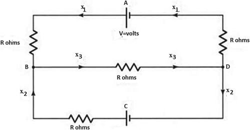
JUNCTIONS:

B: $x_1+x_2=-x_3$

D: $-x_3=x_1+x_2$

A single linear equation is produced by these two equations: $x_1+x_2+x_3=〈(15,18,21)(11,18,25)〉$PATHS:

ABDA: $4x_1+x_3=〈(37,42,47)(31,42,53)〉$

CBDC: $4x_2+x_3=〈(13,18,23)(7,18,29)〉$

A system of three linear equations with three unknowns is known to exist. Therefore, the issue can be solved by solving the system of three linear equations in three variables as follows:

Consider TIFLSEs-I is $\begin{array}{rl}{x}_1+x_2+x_3& =〈(15,18,21)(11,18,25)〉,\\ 4x_1+x_3& =〈(37,42,47)(31,42,53)〉,\\ 4x_2+x_3& =〈(13,18,23)(7,18,29)〉,\end{array}$and $[b_1{]}_{({\sigma }_1,{\sigma }_2)}=〈\left[b_1^{{\text{L}}^{\ast }},b_1^{{\text{U}}^{\ast }}\right],\left[b_1^{\text{L}},b_1^{\text{U}}\right]〉,$ $\begin{array}{rl}[b_2{]}_{({\sigma }_1,{\sigma }_2)}& =〈\left[b_2^{{\text{L}}^{\ast }},b_2^{{\text{U}}^{\ast }}\right],\left[b_2^{\text{L}},b_2^{\text{U}}\right]〉,\\ [x_1{]}_{({\sigma }_1,{\sigma }_2)}& =〈\left[x_1^{{\text{L}}^{\ast }},x_1^{{\text{U}}^{\ast }}\right],\left[x_1^{\text{L}},x_1^{\text{U}}\right]〉,\\ [x_2{]}_{({\sigma }_1,{\sigma }_2)}& =〈\left[x_2^{{\text{L}}^{\ast }},x_2^{{\text{U}}^{\ast }}\right],\left[x_2^{\text{L}},x_2^{\text{U}}\right]〉\end{array}$and $[x_3{]}_{({\sigma }_1,{\sigma }_2)}=〈\left[x_3^{{\text{L}}^{\ast }},x_3^{{\text{U}}^{\ast }}\right],\left[x_3^{\text{L}},x_3^{\text{U}}\right]〉.$

Thus, parametric form of the above system is $\{\begin{array}{rl}& 〈\left[x_1^{{\text{L}}^{\ast }},x_1^{U_1}\right],\left[x_1^L,x_1^U\right]〉+〈\left[x_2^{{\text{L}}^{\ast }},x_2^{U_1}\right],\left[x_2^L,x_2^U\right]〉+〈\left[x_3^{{\text{L}}^{\ast }},x_3^{U_1}\right],\left[x_3^L,x_3^U\right]〉\\ & =〈\left[15+3{\sigma }_1,21-3{\sigma }_1\right],\left[18-7{\sigma }_2,18+7{\sigma }_2\right]〉\\ & 4〈\left[x_1^{{\text{L}}^{\ast }},x_1^{U_1}\right],\left[x_1^L,x_1^U\right]〉+〈\left[x_3^{{\text{L}}^{\ast }},x_3^{U_1}\right],\left[x_3^L,x_3^U\right]〉\\ & =〈\left[37+5{\sigma }_1,47-5{\sigma }_1\right],\left[42-11{\sigma }_2,42+11{\sigma }_2\right]〉\\ & 4〈\left[x_2^{{\text{L}}^{\ast }},x_2^{U_1}\right],\left[x_2^L,x_2^U\right]〉+〈\left[x_3^{{\text{L}}^{\ast }},x_3^{U_1}\right],\left[x_3^L,x_3^U\right]〉\\ & =〈\left[13+5{\sigma }_1,23-5{\sigma }_1\right],\left[18-11{\sigma }_2,18+11{\sigma }_2\right]〉\end{array}$The ${\sigma }_1$ -Cut of the TIFLSEs-I is $\{\begin{array}{rl}1\left[x_1^{{\text{L}}^{\ast }},x_1^{U_1}\right]+1\left[x_2^{{\text{L}}^{\ast }},x_2^{U_1}\right]+\left[x_3^{{\text{L}}^{\ast }},x_3^{U_1}\right]& =〈\left[15+3{\sigma }_1,21-3{\sigma }_1\right]〉\\ 4\left[x_1^{{\text{L}}^{\ast }},x_1^{U_1}\right]+1\left[x_3^{L_1},x_3^{U_1}\right]& =〈\left[37+5{\sigma }_1,47-5{\sigma }_1\right]〉\\ 4\left[x_2^{{\text{L}}^{\ast }},x_2^{U_1}\right]+\left[x_3^{L_1},x_3^{U_1}\right]& =〈\left[13+5{\sigma }_1,23-5{\sigma }_1\right]〉\end{array}$or $\{\begin{array}{rl}\left(x_1^{L_1}\right)+\left(x_2^{L_1}\right)+1\left(x_3^{L_1}\right)+0\left(x_1^{U_1}\right)+0\left(x_2^{U_1}\right)+0\left(x_3^{U_1}\right)& =15+3{\sigma }_1\\ 4\left(x_1^{L_1}\right)+0\left(x_2^{L_1}\right)+1\left(x_3^{L_1}\right)+0\left(x_1^{U_1}\right)+0\left(x_2^{U_1}\right)+0\left(x_3^{U_1}\right)& =37+5{\sigma }_1\\ 0\left(x_1^{L_1}\right)+4\left(x_2^{L_1}\right)+1\left(x_3^{L_1}\right)+0\left(x_1^{U_1}\right)+0\left(x_2^{U_1}\right)+0\left(x_3^{U_1}\right)& =13+5{\sigma }_1\\ 0\left(x_1^{L_1}\right)+0\left(x_2^{L_1}\right)+0\left(x_3^{L_1}\right)+\left(x_1^{U_1}\right)+\left(x_2^{U_1}\right)+\left(x_3^{U_1}\right)& =21-3{\sigma }_1\\ 0\left(x_1^{L_1}\right)+0\left(x_2^{L_1}\right)+0\left(x_3^{L_1}\right)+4\left(x_1^{U_1}\right)+0\left(x_2^{U_1}\right)+\left(x_3^{U_1}\right)& =47-5{\sigma }_1\\ 0\left(x_1^{L_1}\right)+0\left(x_2^{L_1}\right)+0\left(x_3^{L_1}\right)+0\left(x_1^{U_1}\right)+4\left(x_2^{U_1}\right)+\left(x_3^{U_1}\right)& =23-5{\sigma }_1\end{array}$In matrix notation the above TIFLSEs-I for ${\sigma }_1-\text{Cut}$ is written as: $\left(\begin{array}{cccccc}1& 1& 1& 0& 0& 0\\ 4& 0& 1& 0& 0& 0\\ 0& 4& 1& 0& 0& 0\\ 0& 0& 0& 1& 1& 1\\ 0& 0& 0& 4& 0& 1\\ 0& 0& 0& 0& 4& 1\end{array}\right)\left(\begin{array}{c}{x}_1^{L_1}\\ x_2^{L_1}\\ x_3^{L_1}\\ x_1^{U_1}\\ x_2^{U_1}\\ x_3^{U_1}\end{array}\right)=\left(\begin{array}{c}15+3{\sigma }_1\\ 37+5{\sigma }_1\\ 13+5{\sigma }_1\\ 21-3{\sigma }_1\\ 47-5{\sigma }_1\\ 23-5{\sigma }_1\end{array}\right).$The exact solution of TIFLSEs-I for ${\sigma }_1-\text{Cut}$ is given as: $\left(\begin{array}{c}{x}_1^{L_1}\\ x_2^{L_1}\\ x_3^{L_1}\\ x_1^{U_1}\\ x_2^{U_1}\\ x_3^{U_1}\end{array}\right)=\left(\begin{array}{cccccc}-\frac{1}{2}& \frac{3}{8}& \frac{1}{8}& 0& 0& 0\\ -\frac{1}{2}& \frac{1}{8}& \frac{3}{8}& 0& 0& 0\\ 2& \frac{-1}{2}& \frac{-1}{2}& 0& 0& 0\\ 0& 0& 0& -\frac{1}{2}& \frac{3}{8}& \frac{1}{8}\\ 0& 0& 0& -\frac{1}{2}& \frac{1}{8}& \frac{3}{8}\\ 0& 0& 0& 2& \frac{-1}{2}& \frac{-1}{2}\end{array}\right)\ast \left(\begin{array}{c}15+3{\sigma }_1\\ 37+5{\sigma }_1\\ 13+5{\sigma }_1\\ 21-3{\sigma }_1\\ 47-5{\sigma }_1\\ 23-5{\sigma }_1\end{array}\right)=\left(\begin{array}{c}8+{\sigma }_1\\ 2+{\sigma }_1\\ 5+{\sigma }_1\\ 10-{\sigma }_1\\ 4-{\sigma }_1\\ 7-{\sigma }_1\end{array}\right).$The ${\sigma }_2$ -Cut of the TIFLSEs-I is ${\displaystyle \{\begin{array}{l}\left[x_1^L,x_1^U\right]+\left[x_2^L,x_2^U\right]-\left[x_3^L,x_3^U\right]=〈\left[18-7{\sigma }_2,18+7{\sigma }_2\right]〉\\ 4\left[x_1^L,x_1^U\right]+1\left[x_3^L,x_3^U\right]=〈\left[42-11{\sigma }_2,42+11{\sigma }_2\right]〉\\ 4\left[x_2^L,x_2^U\right]+\left[x_3^L,x_3^U\right]=〈\left[18-11{\sigma }_2,18+11{\sigma }_2\right]〉\end{array}}$or $\{\begin{array}{rl}\left(x_1^L\right)+\left(x_2^L\right)+\left(x_3^L\right)+0\left(x_1^U\right)+0\left(x_2^U\right)+0\left(x_3^U\right)& =18-7{\sigma }_2\\ 4\left(x_1^L\right)+0\left(x_2^L\right)+1\left(x_3^L\right)+0\left(x_1^U\right)+0\left(x_2^U\right)+0\left(x_3^U\right)& =42-11{\sigma }_2\\ 0\left(x_1^L\right)+4\left(x_2^L\right)+1\left(x_3^L\right)+0\left(x_1^U\right)+0\left(x_2^U\right)+0\left(x_3^U\right)& =18-11{\sigma }_2\\ 0\left(x_1^L\right)+0\left(x_2^L\right)+0\left(x_3^L\right)+\left(x_1^U\right)+\left(x_2^U\right)+\left(x_3^U\right)& =18+7{\sigma }_2\\ 0\left(x_1^L\right)+\left(x_2^L\right)+0\left(x_3^L\right)+4\left(x_1^U\right)+0\left(x_2^U\right)+\left(x_3^U\right)& =42+11{\sigma }_2\\ 0\left(x_1^L\right)+0\left(x_2^L\right)+0\left(x_3^L\right)+\left(x_1^U\right)+4\left(x_2^U\right)+\left(x_3^U\right)& =18+11{\sigma }_2\end{array}$In matrix notation the above TIFLSEs-I for ${\sigma }_2-\text{Cut}$ is written as: $\left(\begin{array}{cccccc}1& 1& 1& 0& 0& 0\\ 4& 0& 1& 0& 0& 0\\ 0& 4& 1& 0& 0& 0\\ 0& 0& 0& 1& 1& 1\\ 0& 0& 0& 4& 0& 1\\ 0& 0& 0& 0& 4& 1\end{array}\right)\left(\begin{array}{c}{x}_1^L\\ x_2^L\\ x_3^L\\ x_1^U\\ x_2^U\\ x_3^U\end{array}\right)=\left(\begin{array}{c}11-7{\sigma }_2\\ 42-11{\sigma }_2\\ 18-11{\sigma }_2\\ 18+7{\sigma }_2\\ 42+11{\sigma }_2\\ 18+11{\sigma }_2\end{array}\right).$The exact solution of TIFLSEs-I for ${\sigma }_2-\text{Cut}$ is given as: $\left(\begin{array}{c}{x}_1^L\\ x_2^L\\ x_3^L\\ x_1^U\\ x_2^U\\ x_3^U\end{array}\right)=\left(\begin{array}{cccccc}-\frac{1}{2}& \frac{3}{8}& \frac{1}{8}& 0& 0& 0\\ -\frac{1}{2}& \frac{1}{8}& \frac{3}{8}& 0& 0& 0\\ 2& \frac{-1}{2}& \frac{-1}{2}& 0& 0& 0\\ 0& 0& 0& -\frac{1}{2}& \frac{3}{8}& \frac{1}{8}\\ 0& 0& 0& -\frac{1}{2}& \frac{1}{8}& \frac{3}{8}\\ 0& 0& 0& 2& \frac{-1}{2}& \frac{-1}{2}\end{array}\right)\ast \left(\begin{array}{c}11-7{\sigma }_2\\ 42-11{\sigma }_2\\ 18-11{\sigma }_2\\ 18+7{\sigma }_2\\ 42+11{\sigma }_2\\ 18+11{\sigma }_2\end{array}\right)=\left(\begin{array}{c}9-2{\sigma }_2\\ 3-2{\sigma }_2\\ 6-3{\sigma }_2\\ 9+2{\sigma }_2\\ 3+2{\sigma }_2\\ 6+3{\sigma }_2\end{array}\right).$The exact solution of TIFLSEs-I with parameter ${\sigma }_{1,}{\sigma }_2$ is given as: $\begin{array}{rl}{X}_1& =[x_1{]}_{({\sigma }_1,{\sigma }_2)}=〈\left[x_1^{L_1},x_1^{U_1}\right],\left[x_1^L,x_1^U\right]〉=〈\left[8+{\sigma }_1,10-{\sigma }_1\right],\left[9-2{\sigma }_2,9+2{\sigma }_2\right]〉\\ X_2& =[x_2{]}_{({\sigma }_1,{\sigma }_2)}=〈\left[x_2^{L_1},x_2^{U_1}\right],\left[x_2^L,x_2^U\right]〉=〈\left[2+{\sigma }_1,4-{\sigma }_1\right],\left[3-2{\sigma }_2,3+2{\sigma }_2\right]〉\end{array}$and $X_3=[x_3{]}_{({\sigma }_1,{\sigma }_2)}=〈\left[x_3^{L_1},x_3^{U_1}\right],\left[x_3^L,x_3^U\right]〉=〈\left[5+{\sigma }_1,7-{\sigma }_1\right],\left[6-3{\sigma }_2,6+3{\sigma }_2\right]〉$We apply HPM by taking $\begin{array}{rl}\stackrel{`}{\text{U}}& =\left(\begin{array}{cccccc}1& 1& 1& 0& 0& 0\\ 4& 0& 1& 0& 0& 0\\ 0& 4& 1& 0& 0& 0\\ 0& 0& 0& 1& 1& 1\\ 0& 0& 0& 4& 0& 1\\ 0& 0& 0& 0& 4& 1\end{array}\right),\\ \text{Y}{}_{\sigma 1}& =\left(\begin{array}{c}15+3{\sigma }_1\\ 37+5{\sigma }_1\\ 13+5{\sigma }_1\\ 21-3{\sigma }_1\\ 47-5{\sigma }_1\\ 23-5{\sigma }_1\end{array}\right),\\ \text{Y}{}_{\sigma 2}& =\left(\begin{array}{c}11-7{\sigma }_2\\ 42-11{\sigma }_2\\ 18-11{\sigma }_2\\ 18+7{\sigma }_2\\ 42+11{\sigma }_2\\ 18+11{\sigma }_2\end{array}\right),\\ {\hat{\text{G}}}_{\sigma }& =\left(\begin{array}{cccccc}1& 1& 1& 0& 0& 0\\ 4& 0& 1& 0& 0& 0\\ 0& 4& 1& 0& 0& 0\\ 0& 0& 0& 1& 1& 1\\ 0& 0& 0& 4& 0& 1\\ 0& 0& 0& 0& 4& 1\end{array}\right),\\ E_0^L& =\left(\begin{array}{c}8.12+1.02{\sigma }_1\\ 2.21+1.24{\sigma }_1\\ 5.45+1.47{\sigma }_1\\ 10.12-1.34{\sigma }_1\\ 4.52-1.47{\sigma }_1\\ 7.34-1.78{\sigma }_1\end{array}\right),\\ E_0^U& =\left(\begin{array}{c}9.11-2.02{\sigma }_2\\ 3.01-2.04{\sigma }_2\\ 6.01-3.12{\sigma }_2\\ 9.12+2.02{\sigma }_2\\ 3.014+2.01{\sigma }_2\\ 6.01+3.1023{\sigma }_2\end{array}\right).\end{array}$

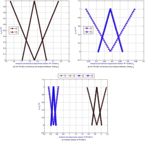
Figure 3(a–d) clearly demonstrates that the numerical approximate solutions obtained by MBHPM are exactly matched with analytical solutions of these systems of equations.

Approximate solution of the TIFLSEs-I obtained by HAM after four iterations is $\begin{array}{rl}{X}_{{\sigma }_1}& =\left(\begin{array}{c}8.00000+1.0000{\sigma }_1\\ 2.00000+1.0000{\sigma }_1\\ 5.00000+1.0000{\sigma }_1\\ 10.0000-1.0000{\sigma }_1\\ 4.0000-1.0000{\sigma }_1\\ 7.0000-1.0000{\sigma }_1\end{array}\right),\\ X_{\sigma 2}& =\left(\begin{array}{c}9.00001-2.0000{\sigma }_2\\ 3.00000-2.0000{\sigma }_2\\ 6.0000-3.0000{\sigma }_2\\ 9.0000+2.0000{\sigma }_2\\ 3.0000+2.0000{\sigma }_2\\ 6.0000+3.0000{\sigma }_2\end{array}\right).\end{array}$In the Jacobi and Gauss-Seidel methods, the desired accuracy of the solutions with $\in ={10}^{-5}$ is obtained after 25 iterations, however in the HPM approach, we obtain an estimated solution up to 25 decimal places after five iterations. The exact solution of the TFLSEs without ${\sigma }_{1,}{\sigma }_2-\mathrm{Cut}$ is given as: $\begin{array}{rl}{\xi }_{{\ddot{e}}_m}^{\ast }\left(x_1\right)& =\{\begin{array}{ll}{\displaystyle \frac{x-8}{1}}& \text{if }8<x<9\\ 1& \text{if }x\in [9,9]\\ {\displaystyle \frac{x-10}{-1}}& 9<x<10\\ 0& \text{otherwise}.\end{array},\\ {\xi }_{{\ddot{e}}_n}\left(x_1\right)& =\{\begin{array}{ll}{\displaystyle \frac{9-x}{2}}& \text{if }7<x<9\\ 1& \text{if }x\in [9,9]\\ {\displaystyle \frac{9-x}{-2}}& 9<x<11\\ 0& \text{otherwise}.\end{array}\\ {\xi }_{{\ddot{e}}_m}^{\ast }\left(x_2\right)& =\{\begin{array}{ll}{\displaystyle \frac{x-2}{1}}& \text{if }2<x<3\\ 1& \text{if }x\in [3,3]\\ {\displaystyle \frac{x-4}{-1}}& 3<x<4\\ 0& \text{otherwise}.\end{array},\\ {\xi }_{{\ddot{e}}_n}\left(x_2\right)& =\{\begin{array}{ll}{\displaystyle \frac{3-x}{2}}& \text{if }1<x<3\\ 1& \text{if }x\in [3,3]\\ {\displaystyle \frac{3-x}{-2}}& 3<x<5\\ 0& \text{otherwise}.\end{array}\\ {\xi }_{{\ddot{e}}_m}^{\ast }\left(x_3\right)& =\{\begin{array}{ll}{\displaystyle \frac{x-5}{1}}& \text{if }5<x<6\\ 1& \text{if }x\in [6,6]\\ {\displaystyle \frac{x-7}{-1}}& 6<x<7\\ 0& \text{otherwise}.\end{array},\end{array}$A method is said to be stable when the solution it produces is unaffected by minor changes in the inputs and parameters and when it is anticipated that such changes will have an influence on the equations and conditions. In this study, we suggested comparing the BHMPM with other existing approaches, such as GSM and JCM, by providing examples and examining the stability of the BHMPM.

Figure 3. (a–d): Shows example 1's semi-numerical TIFLSEs-I solution. (a) solution represents for TIF variables $x_1$, (b) the numerical and analytical approximate solutions for the TIF variable $x_2$, (c) the numerical and analytical approximate solutions for the TIF variables $x_3$, (d) the numerical and analytical approximate solutions for the TIFLSEs-I.

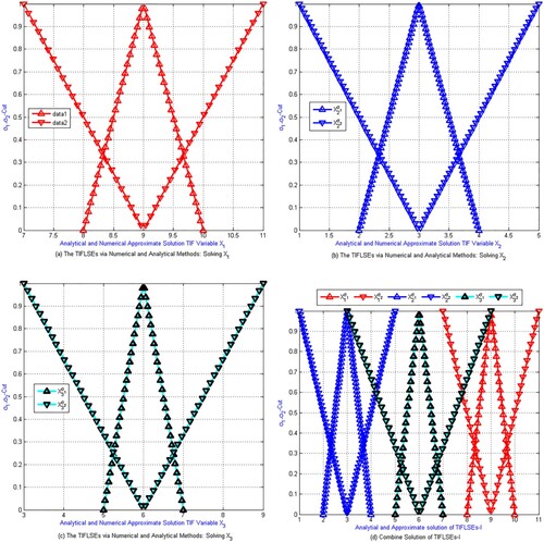
Table 2 compares numerically the computational time seconds (CPU-time), number of iterations (NS), and residual error (ERR) of BHMPM, GSM, JCM, ADMM and SORM for handling engineering applications. We can conclude from Table 2 that the BHMPM has better convergence behaviour and is more stable than the GGSM, JCM, ADMM and SORM technique. We examine the fuzzy linear system equation's solutions while perturbing the fuzzy linear system's alpha-parameter. In comparison to the previous numerical and semi-analytical solutions, the homotopy block technique provides the better approximate solutions starting with the initial solution.

Table 2. Residual error comparison of semi-analytical and numerical schemes for solving TIFLSEs-I.

Parameter	BHMPM	GSM	JCM	ADMM	SORM
CPU-time	0.001	0.013	0.135	0.024	0.015
NS	04.0	20.0	18.0	08.0	15.0
ERR	9.11E-0065	3.52E-009	1.35E-007	2.14E-015	3.14E-006

Example 2:

Consider TIFLSEs-II is $\begin{array}{rl}4x_1-5x_2& =〈(4,5,6)(3,5,7)〉\\ 3x_1+7x_2& =〈(8,9,10)(7,9,11)〉\end{array}$and $[b_1{]}_{({\sigma }_1,{\sigma }_2)}=〈\left[b_1^{L_1},b_1^{U_1}\right],\left[b_1^{\text{L}},b_1^{\text{U}}\right]〉,[b_2{]}_{({\sigma }_1,{\sigma }_2)}=〈\left[b_2^{L_1},b_2^{U_1}\right],\left[b_2^{\text{L}},b_2^{\text{U}}\right]〉,[x_1{]}_{({\sigma }_1,{\sigma }_2)}=〈\left[x_1^{L_1},x_1^{U_1}\right],\left[x_1^{\text{L}},x_1^{\text{U}}\right]〉$ and $[x_2{]}_{({\sigma }_1,{\sigma }_2)}=〈\left[x_2^{{\text{L}}^{\ast }},x_2^{{\text{U}}^{\ast }}\right],\left[x_2^{\text{L}},x_2^{\text{U}}\right]〉.$ Thus, $\{\begin{array}{rl}& 4〈\left[x_1^{L_1},x_1^{U_1}\right],\left[x_1^L,x_1^U\right]〉-5〈\left[x_2^{L_1},x_2^{U_1}\right],\left[x_2^L,x_2^U\right]〉\\ & =〈\left[4+{\sigma }_1,6-{\sigma }_1\right],\left[5-2{\sigma }_2,5+2{\sigma }_2\right]〉,\\ & 3〈\left[x_1^{L_1},x_1^{U_1}\right],\left[x_1^L,x_1^U\right]〉+7〈\left[x_2^{L_1},x_2^{U_1}\right],\left[x_2^L,x_2^U\right]〉\\ & =〈\left[8+{\sigma }_1,10-{\sigma }_1\right],\left[9-2{\sigma }_2,9+2{\sigma }_2\right]〉.\end{array}$The ${\sigma }_1$ -Cut of the TIFLSEs-II is $\{\begin{array}{rl}4\left[x_1^{L_1},x_1^{U_1}\right]-5\left[x_2^{L_1},x_2^{U_1}\right]& =〈\left[4+{\sigma }_1,6-{\sigma }_1\right]〉,\\ 3\left[x_1^{L_1},x_1^{U_1}\right]+7\left[x_2^{L_1},x_2^{U_1}\right]& =〈\left[8+{\sigma }_1,10-{\sigma }_1\right]〉,\end{array}$or $\{\begin{array}{rl}4\left(x_1^{L_1}\right)+0\left(x_2^{L_1}\right)+0\left(x_1^{U_1}\right)+5\left(x_2^{U_1}\right)& =4+{\sigma }_1,\\ 3\left(x_1^{L_1}\right)+7\left(x_2^{L_1}\right)+0\left(x_1^{U_1}\right)+0\left(x_2^{U_1}\right)& =8+{\sigma }_1,\\ 0\left(x_1^{L_1}\right)+5\left(x_2^{L_1}\right)+4\left(x_1^{U_1}\right)+0\left(x_2^{U_1}\right)& =6-{\sigma }_1,\\ 0\left(x_1^{L_1}\right)+0\left(x_2^{L_1}\right)+3\left(x_1^{U_1}\right)+7\left(x_2^{U_1}\right)& =10-{\sigma }_1.\end{array}$In matrix notation the above TIFLSEs-II for ${\sigma }_1-\text{Cut}$ is written as: $\left(\begin{array}{cccc}4& 0& 0& 5\\ 3& 7& 0& 0\\ 0& 5& 4& 0\\ 0& 0& 3& 7\end{array}\right)\left(\begin{array}{c}{x}_1^{L_1}\\ x_2^{L_1}\\ x_1^{U_1}\\ x_2^{U_1}\end{array}\right)=\left(\begin{array}{c}4+{\sigma }_1\\ 8+{\sigma }_1\\ 6-{\sigma }_1\\ 10-{\sigma }_1\end{array}\right).$The exact solution of TIFLSEs-II for ${\sigma }_1-\text{Cut}$ is given as: $\left(\begin{array}{c}{x}_1^{L_1}\\ x_2^{L_1}\\ x_1^{U_1}\\ x_2^{U_1}\end{array}\right)=\left(\begin{array}{cccc}4& 0& 0& 5\\ 3& 7& 0& 0\\ 0& 5& 4& 0\\ 0& 0& 3& 7\end{array}\right)\left(\begin{array}{c}4+{\sigma }_1\\ 8+{\sigma }_1\\ 6-{\sigma }_1\\ 10-{\sigma }_1\end{array}\right)=\left(\begin{array}{c}\frac{954}{559}+\frac{2}{13}{\sigma }_1\\ \frac{230}{559}+\frac{1}{13}{\sigma }_1\\ \frac{1126}{559}-\frac{1}{13}{\sigma }_1\\ \frac{316}{559}-\frac{2}{13}{\sigma }_1\end{array}\right).$The ${\sigma }_2$ -Cut of the TIFLSEs-II is $\{\begin{array}{rl}4\left[x_1^L,x_1^U\right]-5\left[x_2^L,x_2^U\right]& =〈\left[5-2{\sigma }_2,5+2{\sigma }_2\right]〉,\\ 3\left[x_1^L,x_1^U\right]+7\left[x_2^L,x_2^U\right]& =〈\left[9-2{\sigma }_2,9+2{\sigma }_2\right]〉,\end{array}$or $\{\begin{array}{rl}4\left(x_1^L\right)+0\left(x_2^L\right)+0\left(x_1^U\right)+5\left(x_2^U\right)& =5-2{\sigma }_2,\\ 3\left(x_1^L\right)+7\left(x_2^L\right)+0\left(x_1^U\right)+0\left(x_2^U\right)& =9-2{\sigma }_2,\\ 0\left(x_1^L\right)+5\left(x_2^L\right)+4\left(x_1^U\right)+0\left(x_2^U\right)& =5+2{\sigma }_2,\\ 0\left(x_1^L\right)+0\left(x_2^L\right)+3\left(x_1^U\right)+7\left(x_2^U\right)& =9+2{\sigma }_2.\end{array}$In matrix notation the above TIFLSEs-II for ${\sigma }_1-\text{Cut}$ is written as: $\left(\begin{array}{cccc}4& 0& 0& 5\\ 3& 7& 0& 0\\ 0& 5& 4& 0\\ 0& 0& 3& 7\end{array}\right)\left(\begin{array}{c}{x}_1^L\\ x_2^L\\ x_1^U\\ x_2^U\end{array}\right)=\left(\begin{array}{c}5-2{\sigma }_2\\ 9-2{\sigma }_2\\ 5+2{\sigma }_2\\ 9+2{\sigma }_2\end{array}\right).$The exact solution of TIFLSEs-II for ${\sigma }_2-\text{Cut}$ is given as: $\left(\begin{array}{c}{x}_1^L\\ x_2^L\\ x_1^U\\ x_2^U\end{array}\right)=\left(\begin{array}{cccc}\frac{196}{559}& \frac{-75}{559}& \frac{105}{559}& \frac{-140}{559}\\ \frac{-84}{559}& \frac{112}{559}& \frac{-45}{559}& \frac{60}{559}\\ \frac{105}{559}& \frac{140}{559}& \frac{196}{559}& \frac{-75}{559}\\ \frac{-45}{559}& \frac{60}{559}& \frac{-84}{559}& \frac{112}{559}\end{array}\right)\ast \left(\begin{array}{c}5-2{\sigma }_1\\ 9-2{\sigma }_1\\ 5+2{\sigma }_1\\ 9+2{\sigma }_1\end{array}\right)=\left(\begin{array}{c}\frac{80}{43}-\frac{4}{13}{\sigma }_2\\ \frac{21}{43}-\frac{2}{13}{\sigma }_2\\ \frac{80}{43}+\frac{4}{13}{\sigma }_2\\ \frac{21}{43}+\frac{2}{13}{\sigma }_2\end{array}\right).$Therefore the exact TIFLSEs-II is $X_1=[x_1{]}_{({\sigma }_1,{\sigma }_2)}=〈\left[x_1^{L_1},x_1^{U_1}\right],\left[x_1^L,x_1^U\right]〉=〈\begin{array}{c}\left[\frac{954}{559}+\frac{2}{13}{\sigma }_1,\frac{1126}{559}-\frac{1}{13}{\sigma }_1\right],\\ \left[\frac{80}{43}-\frac{4}{13}{\sigma }_1,\frac{80}{43}+\frac{4}{13}{\sigma }_1\right]\end{array}〉$and $X_2=[x_2{]}_{({\sigma }_1,{\sigma }_2)}=〈\left[x_2^{L_1},x_2^{U_1}\right],\left[x_2^L,x_2^U\right]〉=〈\begin{array}{c}\left[\frac{230}{559}+\frac{1}{13}{\sigma }_1,\frac{316}{559}-\frac{2}{13}{\sigma }_1\right],\\ \left[\frac{21}{43}-\frac{2}{13}{\sigma }_2,\frac{21}{43}+\frac{2}{13}{\sigma }_2\right]\end{array}〉.$We apply BHMPM by taking $\begin{array}{rl}\stackrel{`}{U}& =\left(\begin{array}{cccc}4& 0& 0& 5\\ 3& 7& 0& 0\\ 0& 5& 4& 0\\ 0& 0& 3& 7\end{array}\right),\\ Y_{{\sigma }_1}& =\left(\begin{array}{c}4+{\sigma }_1\\ 8+{\sigma }_1\\ 6-{\sigma }_1\\ 10-{\sigma }_1\end{array}\right),\\ {\text{Y}}_{{\sigma }_2}& =\left(\begin{array}{c}5-2{\sigma }_2\\ 9-2{\sigma }_2\\ 5+2{\sigma }_2\\ 9+2{\sigma }_2\end{array}\right),\\ {\hat{\mathrm{G}}}_{\sigma }& =\left(\begin{array}{cccc}4& -5& 0& 0\\ 3& 7& 0& 0\\ 0& 0& 4& -5\\ 0& 0& 3& 7\end{array}\right),\\ E_0^L& =\left(\begin{array}{c}1.581395349+.2790697674\ast {\sigma }_1\\ 0.4651162791+0.2325581395e-1\ast {\sigma }_1\\ -2.139534884+.2790697674\ast {\sigma }_1\\ -.5116279070+0.2325581395e-1\ast {\sigma }_1\end{array}\right),\\ E_0^U& =\left(\begin{array}{c}-1.860465116+.5581395349\ast {\sigma }_2\\ 0.4883720930+0.4651162791e-1\ast {\sigma }_2\\ 1.860465116+.5581395349\ast {\sigma }_2\\ .4883720930+0.4651162791e-1\ast {\sigma }_2\end{array}\right),\end{array}$Figure 4(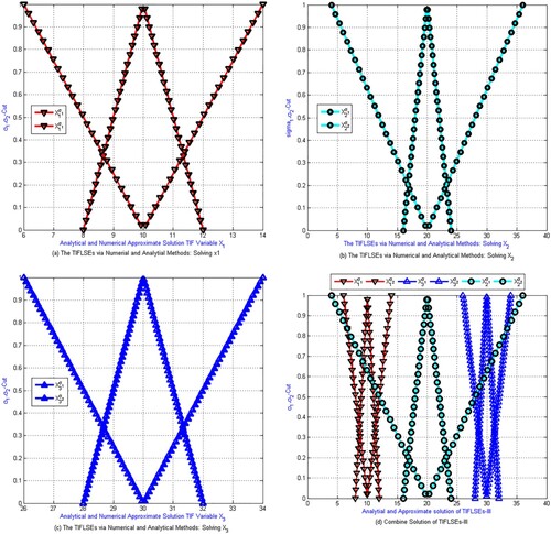a–c), clearly demonstrates that the numerical approximate solutions obtained by MBHPM are exactly matched with analytical solutions of these systems of equations.

Approximate solution of the TILSE-II obtained by BHMPM after four iterations is $\begin{array}{rl}{X}_{{\sigma }_1}& =\left(\begin{array}{c}1.706618962+.1538461538\ast {\sigma }_1\\ .4203200338+0.6805205929e-1{\sigma }_1\\ -2.035010312+.1745451950\ast {\sigma }_1\\ -0.5652951699+0.7692307692e-1\ast {\sigma }_1\end{array}\right),\\ X_{\sigma 2}& =\left(\begin{array}{c}-1.860465116+.3145352711\ast {\sigma }_2\\ -.4883720930+.1509134552\ast {\sigma }_2\\ 1.860465116+0.3145352711\ast {\sigma }_2\\ 0.4883720930+0.1509134552\ast {\sigma }_2\end{array}\right).\end{array}$Figure 4(a–c) clearly illustrates how the analytical and numerical solutions of the TIFLSEs-II employed in Example 2 are exactly matched.

Figure 4. (a–c): Example 2’s semi-numerical TIFLSEs-II solution. (a) solution represents for TIF variables $x_1$, (b) the numerical and analytical approximate solutions for the TIF variable $x_2$, (c) the numerical and analytical approximate solutions for the TIFLSEs-II.

The desired accuracy of the solutions with $\in ={10}^{-7}$ is acquired after 25 iterations and 1.567s, 0.1032s computational CPU-time in the JCM and GSM methods, however in the BHMPM, we obtain an estimated solution up to 30 decimal places i.e. $\in ={10}^{-30}$ after four iterations and 0.011s computational CPU-time. The exact solution of the TFLSEs-II without ${\sigma }_{1,}{\sigma }_2-\mathrm{Cut}$ is given as: $\begin{array}{rl}{\xi }_{{\ddot{e}}_m}^{\ast }\left(x_1\right)& =\{\begin{array}{ll}{\displaystyle \frac{x-{\displaystyle \frac{954}{559}}}{{\displaystyle \frac{2}{13}}}}& \text{if }1.707<x<1.86,\\ 1& \text{if }x\in [1.86,1.86],\\ {\displaystyle \frac{x-{\displaystyle \frac{1126}{559}}}{-{\displaystyle \frac{2}{13}}}}& 1.86<x<2.014,\\ 0& \text{otherwise}.\end{array}\\ {\xi }_{{\ddot{e}}_n}\left(x_1\right)& =\{\begin{array}{ll}{\displaystyle \frac{x-{\displaystyle \frac{80}{43}}}{-{\displaystyle \frac{4}{13}}}}& \text{if }1.557<x<1.86,\\ 1& \text{if }x\in [1.86,1.86],\\ {\displaystyle \frac{x-{\displaystyle \frac{80}{43}}}{{\displaystyle \frac{4}{13}}}}& 1.86<x<2.164,\\ 0& \text{otherwise}.\end{array}\\ {\xi }_{{\ddot{e}}_m}^{\ast }\left(x_2\right)& =\{\begin{array}{ll}{\displaystyle \frac{x-{\displaystyle \frac{230}{559}}}{{\displaystyle \frac{1}{13}}}}& \text{if }0.411<x<0.48,\\ 1& \text{if }x\in [0.48,0.48],\\ {\displaystyle \frac{x-{\displaystyle \frac{316}{559}}}{-{\displaystyle \frac{2}{13}}}}& 0.48<x<0.5653,\\ 0& \mathrm{otherwise}.\end{array}\\ {\xi }_{{\ddot{e}}_n}\left(x_2\right)& =\{\begin{array}{ll}{\displaystyle \frac{x-{\displaystyle \frac{21}{43}}}{-{\displaystyle \frac{2}{13}}}}& \text{if }0.335<x<0.48,\\ 1& \text{if }x\in [21,21],\\ {\displaystyle \frac{x-{\displaystyle \frac{21}{43}}}{{\displaystyle \frac{2}{13}}}}& 0.48<x<0.642,\\ 0& \text{otherwise}.\end{array}\end{array}$Table 3. Shows numerical comparison of computational time seconds (CPU-time), number of iterations (NS) and residual error (ERR) of BHMPM, GSM, JCM, ADMM and SORM respectively for solving TIFLSEs-II. We can conclude from Table 2 that the BHMPM has better convergence behaviour and is more stable than the BHMPM, GSM, JCM, ADMM and SORM technique.

Table 3. Residual error comparison of semi-analytical and numerical schemes for solving TIFLSEs-II.

Parameter	BHMPM	GSM	JCM	ADMM	SORM
CPU-time	0.021	0.103	1.567	0.143	1.467
NS	04.0	25.0	20.0	17.0	16.0
ERR	2.12E-030	3.12E-007	0.32E-05	3.41E-017	0.32E-009

Example 3:

Consider $\begin{array}{rl}2x_1+3x_2-x_3& =〈(128,140,152)(100,140,180)〉\\ 3x_1-x_2+2x_3& =〈(96,110,124)(58,110,168)〉\\ x_1+x_2+x_3& =〈(52,60,68)(36,60,84)〉\end{array}$and $[b_1{]}_{({\sigma }_1,{\sigma }_2)}=〈\left[b_1^{L_1},b_1^{U_1}\right],\left[b_1^{\text{L}},b_1^{\text{U}}\right]〉,[b_2{]}_{({\sigma }_1,{\sigma }_2)}=〈\left[b_2^{L_1},b_2^{U_1}\right],\left[b_2^{\text{L}},b_2^{\text{U}}\right]〉,[x_1{]}_{({\sigma }_1,{\sigma }_2)}=〈\left[x_1^{L_1},x_1^{U_1}\right],\left[x_1^{\text{L}},x_1^{\text{U}}\right]〉$, $[x_2{]}_{({\sigma }_1,{\sigma }_2)}=〈\left[x_2^{{\text{L}}^{\ast }},x_2^{{\text{U}}^{\ast }}\right],\left[x_2^{\text{L}},x_2^{\text{U}}\right]〉.$ and $[x_3{]}_{({\sigma }_1,{\sigma }_2)}=〈\left[x_3^{{\text{L}}^{\ast }},x_3^{{\text{U}}^{\ast }}\right],\left[x_3^{\text{L}},x_3^{\text{U}}\right]〉$.

Thus, $\{\begin{array}{c}2〈\left[x_1^{L_1},x_1^{U_1}\right],\left[x_1^L,x_1^U\right]〉+3〈\left[x_2^{L_1},x_2^{U_1}\right],\left[x_2^L,x_2^U\right]〉-〈\left[x_3^{L_1},x_3^{U_1}\right],\left[x_3^L,x_3^U\right]〉\\ =〈\left[128+12{\sigma }_1,152-12{\sigma }_1\right],\left[140-40{\sigma }_2,140+40{\sigma }_2\right]〉\\ 3〈\left[x_1^{L_1},x_1^{U_1}\right],\left[x_1^L,x_1^U\right]〉-〈\left[x_2^{L_1},x_2^{U_1}\right],\left[x_2^L,x_2^U\right]〉+2〈\left[x_3^{L_1},x_3^{U_1}\right],\left[x_3^L,x_3^U\right]〉\\ =〈\left[96+14{\sigma }_1,124-14{\sigma }_1\right],\left[110-52{\sigma }_2,110+52{\sigma }_2\right]〉\\ 〈\left[x_1^{L_1},x_1^{U_1}\right],\left[x_1^L,x_1^U\right]〉+〈\left[x_2^{L_1},x_2^{U_1}\right],\left[x_2^L,x_2^U\right]〉+〈\left[x_3^{L_1},x_3^{U_1}\right],\left[x_3^L,x_3^U\right]〉\\ =〈\left[52+08{\sigma }_1,68-08{\sigma }_1\right],\left[60-24{\sigma }_2,60+24{\sigma }_2\right]〉\end{array}$The ${\sigma }_1$ -Cut of the TIFLSEs-III is $\{\begin{array}{rl}2\left[x_1^{L_1},x_1^{U_1}\right]+3\left[x_2^{L_1},x_2^{U_1}\right]-\left[x_3^{L_1},x_3^{U_1}\right]& =〈\left[128+12{\sigma }_1,152-12{\sigma }_1\right]〉\\ 3\left[x_1^{L_1},x_1^{U_1}\right]-\left[x_2^{L_1},x_2^{U_1}\right]+2\left[x_3^{L_1},x_3^{U_1}\right]& =〈\left[96+14{\sigma }_1,124-14{\sigma }_1\right]〉\\ \left[x_1^{L_1},x_1^{U_1}\right]+\left[x_2^{L_1},x_2^{U_1}\right]+\left[x_3^{L_1},x_3^{U_1}\right]& =〈\left[52+8{\sigma }_1,68-8{\sigma }_1\right]〉\end{array}$or $\{\begin{array}{rl}2\left(x_1^{L_1}\right)+3\left(x_2^{L_1}\right)+0\left(x_3^{L_1}\right)+0\left(x_1^{U_1}\right)+1\left(x_2^{U_1}\right)+5\left(x_3^{U_1}\right)& =128+12{\sigma }_1\\ 3\left(x_1^{L_1}\right)+0\left(x_2^{L_1}\right)+2\left(x_3^{L_1}\right)+0\left(x_1^{U_1}\right)+1\left(x_2^{U_1}\right)+0\left(x_3^{U_1}\right)& =96+14{\sigma }_1\\ 1\left(x_1^{L_1}\right)+2\left(x_2^{L_1}\right)+3\left(x_3^{L_1}\right)+0\left(x_1^{U_1}\right)+0\left(x_2^{U_1}\right)+0\left(x_3^{U_1}\right)& =52+8{\sigma }_1\\ 0\left(x_1^{L_1}\right)+0\left(x_2^{L_1}\right)+1\left(x_3^{L_1}\right)+2\left(x_1^{U_1}\right)+3\left(x_2^{U_1}\right)+0\left(x_3^{U_1}\right)& =152-12{\sigma }_1\\ 0\left(x_1^{L_1}\right)+1\left(x_2^{L_1}\right)+0\left(x_3^{L_1}\right)+3\left(x_1^{U_1}\right)+0\left(x_2^{U_1}\right)+2\left(x_3^{U_1}\right)& =124-14{\sigma }_1\\ 0\left(x_1^{L_1}\right)+0\left(x_2^{L_1}\right)+0\left(x_3^{L_1}\right)+1\left(x_1^{U_1}\right)+2\left(x_2^{U_1}\right)+3\left(x_3^{U_1}\right)& =68-8{\sigma }_1\end{array}$In matrix notation the above TIFLSEs-III for ${\sigma }_1-\mathrm{Cut}$ is written as: $\left(\begin{array}{cccccc}2& 3& 0& 0& 0& 1\\ 3& 0& 2& 0& 1& 0\\ 1& 2& 3& 0& 0& 0\\ 0& 0& 1& 2& 3& 0\\ 0& 1& 0& 3& 0& 2\\ 0& 0& 0& 1& 2& 3\end{array}\right)\left(\begin{array}{c}{x}_1^{L_1}\\ x_2^{L_1}\\ x_3^{L_1}\\ x_1^{U_1}\\ x_2^{U_1}\\ x_3^{U_1}\end{array}\right)=\left(\begin{array}{c}128+12{\sigma }_1\\ 96+14{\sigma }_1\\ 52+08{\sigma }_1\\ 152-12{\sigma }_1\\ 124-14{\sigma }_1\\ 068-08{\sigma }_1\end{array}\right).$The exact solution of TIFLSEs-III for ${\sigma }_1-\text{Cut}$ is given as: $\begin{array}{rl}\left(\begin{array}{c}{x}_1^{L_1}\\ x_2^{L_1}\\ x_3^{L_1}\\ x_1^{U_1}\\ x_2^{U_1}\\ x_3^{U_1}\end{array}\right)& =\left(\begin{array}{cccccc}\frac{11}{39}& \frac{-19}{39}& \frac{-40}{39}& \frac{-2}{39}& \frac{7}{39}& \frac{-25}{39}\\ \frac{8}{39}& \frac{-11}{39}& \frac{17}{39}& \frac{5}{39}& \frac{-2}{39}& \frac{-4}{39}\\ \frac{-19}{39}& \frac{-8}{39}& \frac{62}{39}& \frac{-7}{39}& \frac{-5}{39}& \frac{29}{39}\\ \frac{2}{39}& \frac{7}{39}& \frac{-25}{39}& \frac{11}{39}& \frac{19}{39}& \frac{-40}{39}\\ \frac{5}{39}& \frac{-2}{39}& \frac{-4}{39}& \frac{8}{39}& \frac{-11}{39}& \frac{17}{39}\\ \frac{-7}{39}& \frac{-5}{39}& \frac{29}{39}& \frac{19}{39}& \frac{-8}{39}& \frac{62}{39}\end{array}\right)\ast \left(\begin{array}{c}128+12{\sigma }_1\\ 96+14{\sigma }_1\\ 52+08{\sigma }_1\\ 152-12{\sigma }_1\\ 124-14{\sigma }_1\\ 068-08{\sigma }_1\end{array}\right)\\ & =\left(\begin{array}{c}16+4{\sigma }_1\\ 28+2{\sigma }_1\\ 8+2{\sigma }_1\\ 24-4{\sigma }_1\\ 32-2{\sigma }_1\\ 12-2{\sigma }_1\end{array}\right).\end{array}$The ${\sigma }_2$ -Cut of the TIFLSEs-III is $\{\begin{array}{rl}2\left[x_1^L,x_1^U\right]+3\left[x_2^L,x_2^U\right]-\left[x_3^L,x_3^U\right]& =〈\left[140-40{\sigma }_2,140+40{\sigma }_2\right]〉\\ 3\left[x_1^L,x_1^U\right]-\left[x_2^L,x_2^U\right]+2\left[x_3^L,x_3^U\right]& =〈\left[110-52{\sigma }_2,110+52{\sigma }_2\right]〉\\ \left[x_1^L,x_1^U\right]+\left[x_2^L,x_2^U\right]+\left[x_3^L,x_3^U\right]& =〈\left[60-24{\sigma }_2,60+24{\sigma }_2\right]〉\end{array}$or $\{\begin{array}{rl}2\left(x_1^L\right)+3\left(x_2^L\right)+0\left(x_3^L\right)+0\left(x_1^U\right)+1\left(x_2^U\right)+5\left(x_3^U\right)& =140-40{\sigma }_2\\ 3\left(x_1^L\right)+0\left(x_2^L\right)+2\left(x_3^L\right)+0\left(x_1^U\right)+1\left(x_2^U\right)+0\left(x_3^U\right)& =110-52{\sigma }_2\\ 1\left(x_1^L\right)+2\left(x_2^L\right)+3\left(x_3^L\right)+0\left(x_1^U\right)+0\left(x_2^U\right)+0\left(x_3^U\right)& =60-24{\sigma }_2\\ 0\left(x_1^L\right)+0\left(x_2^L\right)+1\left(x_3^L\right)+2\left(x_1^U\right)+3\left(x_2^U\right)+0\left(x_3^U\right)& =140+40{\sigma }_2\\ 0\left(x_1^L\right)+1\left(x_2^L\right)+0\left(x_3^L\right)+3\left(x_1^U\right)+0\left(x_2^U\right)+2\left(x_3^U\right)& =110+52{\sigma }_2\\ 0\left(x_1^L\right)+0\left(x_2^L\right)+0\left(x_3^L\right)+1\left(x_1^U\right)+2\left(x_2^U\right)+3\left(x_3^U\right)& =60+24{\sigma }_2\end{array}$In matrix notation the above TIFLSEs-III for ${\sigma }_2-\text{Cut}$ is written as: $\left(\begin{array}{cccccc}2& 3& 0& 0& 0& 1\\ 3& 0& 2& 0& 1& 0\\ 1& 2& 3& 0& 0& 0\\ 0& 0& 1& 2& 3& 0\\ 0& 1& 0& 3& 0& 2\\ 0& 0& 0& 1& 2& 3\end{array}\right)\left(\begin{array}{c}{x}_1^L\\ x_2^L\\ x_3^L\\ x_1^U\\ x_2^U\\ x_3^U\end{array}\right)=\left(\begin{array}{c}140-40{\sigma }_2\\ 110-52{\sigma }_2\\ 60-24{\sigma }_2\\ 140+40{\sigma }_2\\ 110+52{\sigma }_2\\ 60+24{\sigma }_2\end{array}\right).$The exact solution of TIFLSEs-III for ${\sigma }_2-\text{Cut}$ is given as: $\begin{array}{rl}\left(\begin{array}{c}{x}_1^L\\ x_2^L\\ x_3^L\\ x_1^U\\ x_2^U\\ x_3^U\end{array}\right)& =\left(\begin{array}{cccccc}\frac{11}{39}& \frac{-19}{39}& \frac{-40}{39}& \frac{-2}{39}& \frac{7}{39}& \frac{-25}{39}\\ \frac{8}{39}& \frac{-11}{39}& \frac{17}{39}& \frac{5}{39}& \frac{-2}{39}& \frac{-4}{39}\\ \frac{-19}{39}& \frac{-8}{39}& \frac{62}{39}& \frac{-7}{39}& \frac{-5}{39}& \frac{29}{39}\\ \frac{2}{39}& \frac{7}{39}& \frac{-25}{39}& \frac{11}{39}& \frac{19}{39}& \frac{-40}{39}\\ \frac{5}{39}& \frac{-2}{39}& \frac{-4}{39}& \frac{8}{39}& \frac{-11}{39}& \frac{17}{39}\\ \frac{-7}{39}& \frac{-5}{39}& \frac{29}{39}& \frac{19}{39}& \frac{-8}{39}& \frac{62}{39}\end{array}\right)\ast \left(\begin{array}{c}140-40{\sigma }_2\\ 110-52{\sigma }_2\\ 60-24{\sigma }_2\\ 140+40{\sigma }_2\\ 110+52{\sigma }_2\\ 60+24{\sigma }_2\end{array}\right)\\ & =\left(\begin{array}{c}20-16{\sigma }_2\\ 30-4{\sigma }_2\\ 10-4{\sigma }_2\\ 20+16{\sigma }_2\\ 30+4{\sigma }_2\\ 10+4{\sigma }_2\end{array}\right).\end{array}$Figure 5(a–d), clearly demonstrates that the numerical approximate solutions obtained by MBHPM are exactly matched with analytical solutions of these systems of equations.

Figure 5. (a–d): Example 3’s semo-numerical TIFLSEs-III solution (a) solution represents forTIF variables $x_1$, (b) the numerical and analytical approximate solutions for the TIF variable $x_2$, (c) the numerical and analytical approximate solutions for the TIF variables $x_3$, (d) the numerical and analytical approximate solutions for the TIFLSEs-III.

The exact solution of TIFLSEs-II with parameter ${\sigma }_{1,}{\sigma }_2$ is given as: $\begin{array}{rl}{X}_1& =[x_1{]}_{({\sigma }_1,{\sigma }_2)}=〈\left[x_1^{L_1},x_1^{U_1}\right],\left[x_1^L,x_1^U\right]〉\\ & =〈\left[16+4{\sigma }_1,24-4{\sigma }_1\right],\left[20-16{\sigma }_1,20+16{\sigma }_1\right]〉,\\ X_2& =[x_2{]}_{({\sigma }_1,{\sigma }_2)}=〈\left[x_2^{L_1},x_2^{U_1}\right],\left[x_2^L,x_2^U\right]〉\\ & =〈\left[28+8{\sigma }_1,32-2{\sigma }_1\right],\left[30-4{\sigma }_2,30+4{\sigma }_2\right]〉\end{array}$and $X_3=[x_3{]}_{({\sigma }_1,{\sigma }_2)}=〈\left[x_3^{L_1},x_3^{U_1}\right],\left[x_3^L,x_3^U\right]〉=〈\left[8+2{\sigma }_1,8-2{\sigma }_1\right],\left[10-4{\sigma }_2,10+4{\sigma }_2\right]〉.$We apply BHMPM by taking $\begin{array}{rl}\stackrel{`}{\text{U}}& =\left(\begin{array}{cccccc}2& 3& -1& 0& 0& 0\\ 3& -1& 2& 0& 0& 0\\ 1& 2& 3& 0& 0& 0\\ 0& 0& 0& 2& 3& -1\\ 0& 0& 0& 3& -1& 2\\ 0& 0& 0& 1& 2& 3\end{array}\right),\\ \text{Y}{}_{\sigma 1}& =\left(\begin{array}{c}128+12{\sigma }_1\\ 96+14{\sigma }_1\\ 52+08{\sigma }_1\\ 152-12{\sigma }_1\\ 124-14{\sigma }_1\\ 068-08{\sigma }_1\end{array}\right),\\ \text{Y}{}_{\sigma 2}& =\left(\begin{array}{c}140-40{\sigma }_2\\ 110-52{\sigma }_2\\ 60-24{\sigma }_2\\ 140+40{\sigma }_2\\ 110+52{\sigma }_2\\ 60+24{\sigma }_2\end{array}\right),\end{array}$ $\begin{array}{rl}{\hat{\mathrm{G}}}_{\sigma }& =\left(\begin{array}{cccccc}2& 3& 0& 0& 0& 1\\ 3& 0& 2& 0& 1& 0\\ 1& 2& 3& 0& 0& 0\\ 0& 0& 1& 2& 3& 0\\ 0& 1& 0& 3& 0& 2\\ 0& 0& 0& 1& 2& 3\end{array}\right),\\ E_0^L& =\left(\begin{array}{c}40.28571429+4.714285714\ast {\sigma }_1\\ 14.0+{\sigma }_1\\ -5.428571429+.4285714286\ast {\sigma }_1\\ 49.71428571-4.714285714\ast {\sigma }_1\\ 16.0-1.\ast {\sigma }_1\\ -4.571428571-0.4285714286\ast {\sigma }_1\end{array}\right),\\ E_0^U& =\left(\begin{array}{c}-6.7857+.44218\ast {\sigma }_2\\ 7.5000-.61905\ast {\sigma }_2\\ -1.0714-.97279\ast {\sigma }_2\\ -6.7857-.44218\ast {\sigma }_2\\ 7.5000+.61905\ast {\sigma }_2\\ -1.0714+.97279\ast {\sigma }_2\end{array}\right).\end{array}$Approximate solution of the TIFLSEs-III obtained by BHMPM after four iterations is $\begin{array}{rl}{X}_{{\sigma }_1}& =\left(\begin{array}{c}16.733+4.0004\ast {\sigma }_1\\ \mathrm{.28.001}+1.9994\ast {\sigma }_1\\ 6.9014+1.9991\ast {\sigma }_1\\ 24.733-4.0004\ast {\sigma }_1\\ 31.999-1.9994\ast {\sigma }_1\\ 10.900-1.9991\ast {\sigma }_1\end{array}\right),\\ X_{\sigma 2}& =\left(\begin{array}{c}20.733-16.001\ast {\sigma }_2\\ 30.000-3.9988\ast {\sigma }_2\\ 09.900-3.9980\ast {\sigma }_2\\ 20.733+16.001\ast {\sigma }_2\\ 30.000+3.9988\ast {\sigma }_2\\ 09.900+3.9980\ast {\sigma }_2\end{array}\right).\end{array}$The desired accuracy of the solutions with $\in ={10}^{-5}$ is acquired after 25 iterations and 1.567s, 1.032s computational CPU-time in the JCM and GSM methods, however, in the BHMPM method, we obtain an estimated solution up to 30 decimal places i.e. $\in ={10}^{-30}$ after four iterations and 0.011s computational CPU-time. The exact solution of the TFLSEs-III without ${\sigma }_{1,}{\sigma }_2-\text{Cut}$ is given as: $\begin{array}{rl}{\xi }_{{\ddot{e}}_m}^{\ast }\left(x_1\right)& =\{\begin{array}{ll}{\displaystyle \frac{x-8}{2}}& \text{if }08<x<10,\\ 1& \text{if }x\in [10,10],\\ {\displaystyle \frac{x-12}{-2}}& 10<x<12,\\ 0& \text{otherwise}.\end{array},\\ {\xi }_{{\ddot{e}}_n}\left(x_1\right)& =\{\begin{array}{ll}{\displaystyle \frac{10-x}{4}}& \text{if }6<x<10,\\ 1& \text{if }x\in [10,10],\\ {\displaystyle \frac{10-x}{-4}}& 10<x<14,\\ 0& \text{otherwise}.\end{array}\\ {\xi }_{{\ddot{e}}_m}^{\ast }\left(x_2\right)& =\{\begin{array}{ll}{\displaystyle \frac{x-28}{2}}& \text{if }28<x<30,\\ 1& \text{if }x\in [30,30],\\ {\displaystyle \frac{x-32}{-2}}& 30<x<32,\\ 0& \text{otherwise}.\end{array},\end{array}$ $\begin{array}{rl}{\xi }_{{\ddot{e}}_n}\left(x_2\right)& =\{\begin{array}{ll}{\displaystyle \frac{30-x}{4}}& \text{if }26<x<30,\\ 1& \text{if }x\in [30,30],\\ {\displaystyle \frac{30-x}{-4}}& 30<x<34,\\ 0& \text{otherwise}.\end{array}\\ {\xi }_{{\ddot{e}}_m}^{\ast }\left(x_3\right)& =\{\begin{array}{ll}{\displaystyle \frac{x-16}{4}}& \text{if }16<x<20,\\ 1& \text{if }x\in [20,20],\\ {\displaystyle \frac{x-24}{-4}}& 20<x<24,\\ 0& \text{otherwise}.\end{array},\\ {\xi }_{{\ddot{e}}_n}\left(x_3\right)& =\{\begin{array}{ll}{\displaystyle \frac{20-x}{4}}& \text{if }4<x<20,\\ 1& \text{if }x\in [20,20],\\ {\displaystyle \frac{20-x}{-4}}& 20<x<36,\\ 0& \text{otherwise}.\end{array}\end{array}$Table 4 compares numerically the computational time seconds (CPU-time), number of iterations (NS), and residual error (ERR) of BHMPM, GSM, and JCM for solving TIFLSEs-III. We can conclude from Table 3 that the BHMPM has better convergence behaviour and is more stable than the GSM and JCM technique.

Example 4:

Consider TIFLSEs-IV is given as: $\begin{array}{rl}-3x_1+5x_2+7x_3+8x_4+9x_5& =〈\begin{array}{c}(642,874,1106)\\ (572,874,1176)\end{array}〉,\\ 4x_1+5x_2+3x_3+7x_4-1x_5& =〈\begin{array}{c}(502,518,534)\\ (468,518,568)\end{array}〉,\\ 1x_1-2x_2+3x_3+4x_4+5x_5& =〈\begin{array}{c}(300,422,544)\\ (268,422,576)\end{array}〉,\\ 9x_1+8x_2+7x_3+6x_4+5x_5& =〈\begin{array}{c}(608,778,948)\\ (528,778,1028)\end{array}〉,\\ 2x_1+3x_2+7x_3-1x_4+x_5& =〈\begin{array}{c}(306,350,394)\\ (280,350,420)\end{array}〉,\end{array}$and $[b_1{]}_{({\sigma }_1,{\sigma }_2)}=〈\left[b_1^{L_1},b_1^{U_1}\right],\left[b_1^{\text{L}},b_1^{\text{U}}\right]〉,[b_2{]}_{({\sigma }_1,{\sigma }_2)}=〈\left[b_2^{L_1},b_2^{U_1}\right],\left[b_2^{\text{L}},b_2^{\text{U}}\right]〉,[x_1{]}_{({\sigma }_1,{\sigma }_2)}=〈\left[x_1^{L_1},x_1^{U_1}\right],\left[x_1^{\text{L}},x_1^{\text{U}}\right]〉$, $[x_2{]}_{({\sigma }_1,{\sigma }_2)}=〈\left[x_2^{L_1},x_2^{U_1}\right],\left[x_2^{\text{L}},x_2^{\text{U}}\right]〉$, $[x3{]}_{({\sigma }_1,{\sigma }_2)}=〈\left[x_3^{L_1},x_3^{U_1}\right],[x_3^{\text{L}},x_3^{\text{U}}]〉,$ $[x_4{]}_{({\sigma }_1,{\sigma }_2)}=〈\left[x_4^{L_1},x_4^{U_1}\right],\left[x_4^{\text{L}},x_4^{\text{U}}\right]〉$, and $[x_5{]}_{({\sigma }_1,{\sigma }_2)}=〈\left[x_5^{L_1},x_5^{U_1}\right],\left[x_5^{\text{L}},x_5^{\text{U}}\right]〉$ Thus

$\{\begin{array}{rl}& -3〈\left[x_1^L,x_1^U\right],\left[x_1^L,x_1^U\right]〉+5〈\left[x_2^L,x_2^U\right],\left[x_2^L,x_2^U\right]〉+7〈\left[x_3^L,x_3^U\right],\left[x_3^L,x_3^U\right]〉\\ & +8〈\left[x_4^L,x_4^U\right],\left[x_4^L,x_4^U\right]〉+9〈\left[x_5^L,x_5^U\right],\left[x_5^L,x_5^U\right]〉\\ & =〈(642+232{\sigma }_1,1106-232{\sigma }_1)(874-302{\sigma }_2,874+302{\sigma }_2)〉\\ & 4〈\left[x_1^L,x_1^U\right],\left[x_1^L,x_1^U\right]〉+5〈\left[x_2^L,x_2^U\right],\left[x_2^{L^{\ast }},x_2^{U^{\ast }}\right]〉+3〈\left[x_3^L,x_3^U\right],\left[x_3^L,x_3^U\right]〉\\ & +7〈\left[x_4^L,x_4^U\right],\left[x_4^L,x_4^U\right]〉-1〈\left[x_5^L,x_5^U\right],\left[x_5^L,x_5^U\right]〉\\ & =〈(502+16{\sigma }_1,534-16{\sigma }_1)(518-50{\sigma }_2,518+50{\sigma }_2)〉\\ & 1〈\left[x_1^L,x_1^U\right],\left[x_1^L,x_1^U\right]〉-2〈\left[x_2^L,x_2^U\right],\left[x_2^L,x_2^U\right]〉+3〈\left[x_3^L,x_3^U\right],\left[x_3^L,x_3^U\right]〉\\ & +4〈\left[x_4^L,x_4^U\right],\left[x_4^L,x_4^U\right]〉+5〈\left[x_5^L,x_5^U\right],\left[x_5^L,x_5^U\right]〉\\ & =〈(300+122{\sigma }_1,544-122{\sigma }_1)(422-154{\sigma }_2,422+154{\sigma }_2)〉\\ & 9〈\left[x_1^L,x_1^U\right],\left[x_1^L,x_1^U\right]〉+8〈\left[x_2^L,x_2^U\right],\left[x_2^L,x_2^U\right]〉+7〈\left[x_3^L,x_3^U\right],\left[x_3^L,x_3^U\right]〉\\ & +6〈\left[x_4^L,x_4^U\right],\left[x_4^L,x_4^U\right]〉+5〈\left[x_5^L,x_5^U\right],\left[x_5^L,x_5^U\right]〉\\ & =〈(608+170{\sigma }_1,948-170{\sigma }_1)(778-250{\sigma }_2,778+250{\sigma }_2)〉\\ & 2〈\left[x_1^L,x_1^U\right],\left[x_1^L,x_1^U\right]〉+3〈\left[x_2^L,x_2^U\right],\left[x_2^L,x_2^U\right]〉+7〈\left[x_3^L,x_3^U\right],\left[x_3^L,x_3^U\right]〉\\ & -1〈\left[x_4^L,x_4^U\right],\left[x_4^L,x_4^U\right]〉+〈\left[x_5^L,x_5^U\right],\left[x_5^L,x_5^U\right]〉\\ & =〈(306+44{\sigma }_1,394-44{\sigma }_1)(350-70{\sigma }_2,350+70{\sigma }_2)〉\end{array}$The ${\sigma }_1$ -Cut of the TIFLSEs-IV is: $\{\begin{array}{rl}& -3〈\left[x_1^{L_1},x_1^{U_1}\right]〉+5〈\left[x_2^{L_1},x_2^{U_1}\right]〉+7〈\left[x_3^{L_1},x_3^{U_1}\right]〉+8〈\left[x_4^{L_1},x_4^{U_1}\right]〉+9〈\left[x_5^{L_1},x_5^{U_1}\right]〉\\ & =〈(642+232{\sigma }_1,1106-232{\sigma }_1)〉\\ & 4〈\left[x_1^{L_1},x_1^{U_1}\right]〉+5〈\left[x_2^{L_1},x_2^{U_1}\right]〉+3〈\left[x_3^{L_1},x_3^{U_1}\right]〉+7〈\left[x_4^{L_1},x_4^{U_1}\right]〉-1〈\left[x_5^{L_1},x_5^{U_1}\right]〉\\ & =〈(502+16{\sigma }_1,534-16{\sigma }_1)〉\\ & 1〈\left[x_1^{L_1},x_1^{U_1}\right]〉-2〈\left[x_2^{L_1},x_2^{U_1}\right]〉+3〈\left[x_3^{L_1},x_3^{U_1}\right]〉+4〈\left[x_4^{L_1},x_4^{U_1}\right]〉+5〈\left[x_5^{L_1},x_5^{U_1}\right]〉\\ & =〈(300+122{\sigma }_1,544-122{\sigma }_1)〉\\ & 9〈\left[x_1^{L_1},x_1^{U_1}\right]〉+8〈\left[x_2^{L_1},x_2^{U_1}\right]〉+7〈\left[x_3^{L_1},x_3^{U_1}\right]〉+6〈\left[x_4^{L_1},x_4^{U_1}\right]〉+5〈\left[x_5^{L_1},x_5^{U_1}\right]〉\\ & =〈(608+170{\sigma }_1,948-170{\sigma }_1)〉\\ & 2〈\left[x_1^{L_1},x_1^{U_1}\right]〉+3〈\left[x_2^{L_1},x_2^{U_1}\right],〉+7〈\left[x_3^{L_1},x_3^{U_1}\right]〉-1〈\left[x_4^{L_1},x_4^{U_1}\right]〉+〈\left[x_5^{L_1},x_5^{U_1}\right]〉\\ & =〈(306+44{\sigma }_1,394-44{\sigma }_1)〉\end{array}$or $\{\begin{array}{rl}& 0\left(x_1^{L_1}\right)+5\left(x_2^{L_1}\right)+7\left(x_3^{L_1}\right)+8\left(x_4^{L_1}\right)+9x_5^{L_1}+3\left(x_1^{U_1}\right)+0\left(x_2^{U_1}\right)+0\left(x_3^{U_1}\right)\\ & +0\left(x_4^{U_1}\right)+0\left(x_5^{U_1}\right)=642+232{\sigma }_1\\ & 4\left(x_1^{L_1}\right)+5\left(x_2^{L_1}\right)+3\left(x_3^{L_1}\right)+7\left(x_4^{L_1}\right)+0x_5^{L_1}+0\left(x_1^{U_1}\right)+0\left(x_2^{U_1}\right)+0\left(x_3^{U_1}\right)\\ & +0\left(x_4^{U_1}\right)+1\left(x_5^{U_1}\right)=502+16{\sigma }_1\\ & 1\left(x_1^{L_1}\right)+0\left(x_2^{L_1}\right)+3\left(x_3^{L_1}\right)+4\left(x_4^{L_1}\right)+5x_5^{L_1}+0\left(x_1^{U_1}\right)+2\left(x_2^{U_1}\right)+0\left(x_3^{U_1}\right)\\ & +0\left(x_4^{U_1}\right)+0\left(x_5^{U_1}\right)=300+122{\sigma }_1\\ & 9\left(x_1^{L_1}\right)+8\left(x_2^{L_1}\right)+7\left(x_3^{L_1}\right)+6\left(x_4^{L_1}\right)+5x_5^{L_1}+0\left(x_1^{U_1}\right)+0\left(x_2^{U_1}\right)+0\left(x_3^{U_1}\right)\\ & +0\left(x_4^{U_1}\right)+0\left(x_5^{U_1}\right)=608+170{\sigma }_1\\ & 2\left(x_1^{L_1}\right)+3\left(x_2^{L_1}\right)+7\left(x_3^{L_1}\right)+0\left(x_4^{L_1}\right)+1x_5^{L_1}+0\left(x_1^{U_1}\right)+0\left(x_2^{U_1}\right)+0\left(x_3^{U_1}\right)\\ & +1\left(x_4^{U_1}\right)+0\left(x_5^{U_1}\right)=306+44{\sigma }_1\\ & 3\left(x_1^{L_1}\right)+0\left(x_2^{L_1}\right)+0\left(x_3^{L_1}\right)+0\left(x_4^{L_1}\right)+0x_5^{L_1}+0\left(x_1^{U_1}\right)+5\left(x_2^{U_1}\right)+7\left(x_3^{U_1}\right)\\ & +8\left(x_4^{U_1}\right)+9\left(x_5^{U_1}\right)=1106-232{\sigma }_1\\ & 0\left(x_1^{L_1}\right)+0\left(x_2^{L_1}\right)+0\left(x_3^{L_1}\right)+0\left(x_4^{L_1}\right)+1x_5^{L_1}+4\left(x_1^{U_1}\right)+5\left(x_2^{U_1}\right)+3\left(x_3^{U_1}\right)\\ & +7\left(x_4^{U_1}\right)+0\left(x_5^U\right)=534-16{\sigma }_1\\ & 0\left(x_1^{L_1}\right)+2\left(x_2^{L_1}\right)+0\left(x_3^{L_1}\right)+0\left(x_4^{L_1}\right)+0x_5^{L_1}+1\left(x_1^{U_1}\right)+0\left(x_2^{U_1}\right)+3\left(x_3^{U_1}\right)\\ & +4\left(x_4^{U_1}\right)+5\left(x_5^{U_1}\right)=544-122{\sigma }_1\\ & 0\left(x_1^{L_1}\right)+0\left(x_2^{L_1}\right)+0\left(x_3^{L_1}\right)+0\left(x_4^{L_1}\right)+0x_5^{L_1}+9\left(x_1^{U_1}\right)+8\left(x_2^{U_1}\right)+7\left(x_3^{U_1}\right)\\ & +6\left(x_4^{U_1}\right)+5\left(x_5^{U_1}\right)=948-170{\sigma }_1\\ & 0\left(x_1^L\right)+0\left(x_2^L\right)+0\left(x_3^L\right)+1\left(x_4^L\right)+0x_5^L+2\left(x_1^{U_1}\right)+3\left(x_2^{U_1}\right)+7\left(x_3^{U_1}\right)+0\left(x_4^{U_1}\right)\\ & +1\left(x_5^{U_1}\right)=394-44{\sigma }_1\end{array}$In matrix notation the above TIFLSEs-IV for ${\sigma }_1-\mathrm{Cut}$ is written as: $\left(\begin{array}{cccccccccc}0& 5& 7& 8& 9& 3& 0& 0& 0& 0\\ 4& 5& 3& 7& 0& 0& 0& 0& 0& 1\\ 1& 0& 3& 4& 5& 0& 2& 0& 0& 0\\ 9& 8& 7& 6& 5& 0& 0& 0& 0& 0\\ 2& 3& 7& 0& 1& 0& 0& 0& 1& 0\\ 3& 0& 0& 0& 0& 0& 5& 7& 8& 9\\ 0& 0& 0& 0& 1& 4& 5& 3& 7& 0\\ 0& 2& 0& 0& 0& 1& 0& 3& 4& 5\\ 0& 0& 0& 0& 0& 9& 8& 7& 6& 5\\ 0& 0& 0& 1& 0& 2& 3& 7& 0& 1\end{array}\right)\left(\begin{array}{c}{x}_1^{L_1}\\ x_2^{L_1}\\ x_3^{L_1}\\ x_4^{L_1}\\ x_5^{L_1}\\ x_1^{U_1}\\ x_2^{U_1}\\ x_3^{U_1}\\ x_4^{U_1}\\ x_5^{U_1}\end{array}\right)=\left(\begin{array}{c}642+232{\sigma }_1\\ 502+16{\sigma }_1\\ 300+122{\sigma }_1\\ 608+170{\sigma }_1\\ 306+44{\sigma }_1\\ 1106-232{\sigma }_1\\ 534-16{\sigma }_1\\ 544-122{\sigma }_1\\ 948-170{\sigma }_1\\ 394-44{\sigma }_1\end{array}\right).$The exact solution of TIFLSEs-IV for ${\sigma }_1-\mathrm{Cut}$ is given as: $\left(\begin{array}{c}{x}_1^{L_1}\\ x_2^{L_1}\\ x_3^{L_1}\\ x_4^{L_1}\\ x_5^{L_1}\\ x_1^{U_1}\\ x_2^{U_1}\\ x_3^{U_1}\\ x_4^{U_1}\\ x_5^{U_1}\end{array}\right)=A^{-1}\ast \left(\begin{array}{c}642+232{\sigma }_1\\ 502+16{\sigma }_1\\ 300+122{\sigma }_1\\ 608+170{\sigma }_1\\ 306+44{\sigma }_1\\ 1106-232{\sigma }_1\\ 534-16{\sigma }_1\\ 544-122{\sigma }_1\\ 948-170{\sigma }_1\\ 394-44{\sigma }_1\end{array}\right)==\left(\begin{array}{c}4+2{\sigma }_1\\ 14+2{\sigma }_1\\ 30+2{\sigma }_1\\ 40+2{\sigma }_1\\ 2+22{\sigma }_1\\ 8-2{\sigma }_1\\ 18-2{\sigma }_1\\ 34-2{\sigma }_1\\ 44-2{\sigma }_1\\ 46-22{\sigma }_1\end{array}\right)$where $A^{-1}=\left(\begin{array}{ccccc}-\frac{46868}{17301}& \frac{5537}{23068}& \frac{76958}{17301}& \frac{3403}{11534}& \frac{28007}{69204}\\ \frac{84229}{17301}& -\frac{5967}{11534}& -\frac{1423993}{173010}& -\frac{15291}{57670}& -\frac{29555}{34602}\\ -\frac{20279}{17301}& \frac{7173}{46136}& \frac{173359}{86505}& \frac{1297}{115340}& \frac{52351}{138408}\\ -\frac{8624}{5767}& \frac{7281}{23068}& \frac{74568}{28835}& \frac{1331}{57670}& \frac{5277}{23068}\\ \frac{3011}{5767}& -\frac{9261}{46136}& -\frac{4305}{5767}& \frac{1147}{23068}& -\frac{7653}{46136}\\ -\frac{45404}{17301}& \frac{5997}{23068}& \frac{151735}{34602}& \frac{1182}{5767}& \frac{29663}{69204}\\ \frac{83014}{17301}& -\frac{5567}{11534}& -\frac{1390303}{173010}& -\frac{19311}{57670}& -\frac{28115}{34602}\\ -\frac{20090}{17301}& \frac{4361}{46136}& \frac{166894}{86505}& \frac{10237}{115340}& \frac{28387}{138408}\\ -\frac{8677}{5767}& \frac{4253}{23068}& \frac{144981}{57670}& \frac{2218}{28835}& \frac{6257}{23068}\\ \frac{2756}{5767}& -\frac{2273}{46136}& -\frac{8691}{11534}& -\frac{1147}{23068}& -\frac{3881}{46136}\\ -\frac{45404}{17301}& \frac{5997}{23068}& -\frac{151735}{34602}& \frac{1182}{5767}& \frac{29663}{69204}\\ \frac{83014}{17301}& -\frac{5567}{11534}& \frac{1390303}{173010}& -\frac{19311}{57670}& -\frac{28115}{34602}\\ -\frac{20090}{17301}& \frac{4361}{46136}& \frac{166894}{86505}& \frac{10237}{115340}& \frac{28387}{138408}\\ -\frac{8677}{5767}& \frac{4253}{23068}& \frac{144981}{57670}& \frac{2218}{28835}& \frac{6257}{23068}\\ \frac{2756}{5767}& -\frac{2273}{46136}& -\frac{8691}{11534}& -\frac{1147}{23068}& -\frac{3881}{46136}\\ -\frac{46868}{17301}& \frac{5537}{23068}& \frac{76958}{17301}& \frac{3403}{11534}& \frac{28007}{69204}\\ \frac{84229}{17301}& -\frac{5967}{11534}& -\frac{1423993}{173010}& -\frac{15291}{57670}& -\frac{29555}{34602}\\ -\frac{20279}{17301}& \frac{7173}{46136}& \frac{173359}{86505}& \frac{1297}{115340}& \frac{52351}{138408}\\ -\frac{8624}{5767}& \frac{7281}{23068}& \frac{74568}{28835}& \frac{1331}{57670}& \frac{5277}{23068}\\ \frac{3011}{5767}& -\frac{9261}{46136}& -\frac{4305}{5767}& \frac{1147}{23068}& -\frac{7653}{46136}\end{array}\right)$The ${\sigma }_2$ -Cut of the TIFLSEs-IV is given as: $\begin{array}{rl}& \{\begin{array}{rl}& -3〈\left[x^L,x_1^U\right],\left[x_1^L,x_1^U\right]〉+5〈\left[x_2^L,x_2^U\right],\left[x_2^L,x_2^U\right]〉+7〈\left[x_3^L,x_3^U\right],\left[x_3^L,x_3^U\right]〉\\ & +8〈\left[x_4^L,x_4^U\right],\left[x_4^L,x_4^U\right]〉+9〈\left[x_5^L,x_5^U\right],\left[x_5^L,x_5^U\right]〉=〈(874-302{\sigma }_2,874+302{\sigma }_2)〉\\ & 4〈\left[x_1^L,x_1^U\right],\left[x_1^L,x_1^U\right]〉+5〈\left[x_2^L,x_2^U\right],\left[x_2^L,x_2^U\right]〉+3〈\left[x_3^{L^{\ast }},x_3^U\right],\left[x_3^L,x_3^U\right]〉\\ & +7〈\left[x_4^L,x_4^U\right],\left[x_4^L,x_4^U\right]〉-1〈\left[x_5^L,x_5^U\right],\left[x_5^L,x_5^U\right]〉=〈(518-50{\sigma }_2,518+50{\sigma }_2)〉\\ & 1〈\left[x_1^L,x_1^U\right],\left[x_1^L,x_1^U\right]〉-2〈\left[x_2^L,x_2^U\right],\left[x_2^L,x_2^U\right]〉+3〈\left[x_3^L,x_3^U\right],\left[x_3^L,x_3^U\right]〉\\ & +4〈\left[x_4^L,x_4^U\right],\left[x_4^L,x_4^U\right]〉+5〈\left[x_5^L,x_5^U\right],\left[x_5^L,x_5^U\right]〉=〈(422-154{\sigma }_2,422+154{\sigma }_2)〉\\ & 9〈\left[x_1^L,x_1^U\right],\left[x_1^L,x_1^U\right]〉+8〈\left[x_2^L,x_2^U\right],\left[x_2^L,x_2^U\right]〉+7〈\left[x_3^L,x_3^U\right],\left[x_3^L,x_3^U\right]〉\\ & +6〈\left[x_4^L,x_4^U\right],\left[x_4^L,x_4^U\right]〉+5〈\left[x_5^L,x_5^U\right],\left[x_5^L,x_5^U\right]〉=〈(778-250{\sigma }_2,778+250{\sigma }_2)〉\\ & 2〈\left[x_1^L,x_1^U\right],\left[x_1^L,x_1^U\right]〉+3〈\left[x_2^L,x_2^U\right],\left[x_2^L,x_2^U\right]〉+7〈\left[x_3^L,x_3^U\right],\left[x_3^L,x_3^U\right]〉\\ & -1〈\left[x_4^L,x_4^U\right],\left[x_4^L,x_4^U\right]〉+〈\left[x_5^L,x_5^U\right],\left[x_5^L,x_5^U\right]〉=〈(350-70{\sigma }_2,350+70{\sigma }_2)〉\end{array}\\ & \{\begin{array}{rl}& -3〈\left[x_1^L,x_1^U\right]〉+5〈\left[x_2^L,x_2^U\right]〉+7〈\left[x_3^L,x_3^U\right]〉+8〈\left[x_4^L,x_4^U\right]〉+9〈\left[x_5^L,x_5^U\right]〉\\ & =〈(874-302{\sigma }_2,874+302{\sigma }_2)〉\\ & 4〈\left[x_1^L,x_1^U\right]〉+5〈\left[x_2^L,x_2^U\right]〉+3〈\left[x_3^L,x_3^U\right]〉+7〈\left[x_4^L,x_4^U\right]〉-1〈\left[x_5^L,x_5^U\right]〉\\ & =〈(518-50{\sigma }_2,518+50{\sigma }_2)〉\\ & 1〈\left[x_1^L,x_1^U\right]〉-2〈\left[x_2^L,x_2^U\right]〉+3〈\left[x_3^L,x_3^U\right]〉+4〈\left[x_4^L,x_4^U\right]〉+5〈\left[x_5^L,x_5^U\right]〉\\ & =〈(422-154{\sigma }_2,422+154{\sigma }_2)〉\\ & 9〈\left[x_1^L,x_1^U\right]〉+8〈\left[x_2^L,x_2^U\right]〉+7〈\left[x_3^L,x_3^U\right]〉+6〈\left[x_4^L,x_4^U\right]〉+5〈\left[x_5^L,x_5^U\right]〉\\ & =〈(778-250{\sigma }_2,778+250{\sigma }_2)〉\\ & 2〈\left[x_1^L,x_1^U\right]〉+3〈\left[x_2^L,x_2^U\right],〉+7〈\left[x_3^L,x_3^U\right]〉-1〈\left[x_4^L,x_4^U\right]〉+〈\left[x_5^L,x_5^U\right]〉\\ & =〈(350-70{\sigma }_2,350+70{\sigma }_2)〉\end{array}\end{array}$or $\{\begin{array}{rl}& 0\left(x_1^L\right)+5\left(x_2^L\right)+7\left(x_3^L\right)+8\left(x_4^L\right)+9\left(x_5^L\right)+3\left(x_1^U\right)+0\left(x_2^U\right)+0\left(x_3^U\right)+0\left(x_4^U\right)+0\left(x_5^U\right)=874-302{\sigma }_2\\ & 4\left(x_1^L\right)+5\left(x_2^L\right)+3\left(x_3^L\right)+7\left(x_4^L\right)+0\left(x_5^L\right)+0\left(x_1^U\right)+0\left(x_2^U\right)+0\left(x_3^U\right)+0\left(x_4^U\right)+1\left(x_5^U\right)=518-50{\sigma }_2\\ & 1\left(x_1^L\right)+0\left(x_2^L\right)+3\left(x_3^L\right)+4\left(x_4^L\right)+5\left(x_5^L\right)+0\left(x_1^U\right)+2\left(x_2^U\right)+0\left(x_3^U\right)+0\left(x_4^U\right)+0\left(x_5^U\right)=422-154{\sigma }_2\\ & 9\left(x_1^L\right)+8\left(x_2^L\right)+7\left(x_3^L\right)+6\left(x_4^L\right)+5\left(x_5^L\right)+0\left(x_1^U\right)+0\left(x_2^U\right)+0\left(x_3^U\right)+0\left(x_4^U\right)+0\left(x_5^U\right)=778-250{\sigma }_2\\ & 2\left(x_1^L\right)+3\left(x_2^L\right)+7\left(x_3^L\right)+0\left(x_4^L\right)+1\left(x_5^L\right)+0\left(x_1^U\right)+0\left(x_2^U\right)+0\left(x_3^U\right)+1\left(x_4^U\right)+0\left(x_5^U\right)=350-70{\sigma }_2\\ & 3\left(x_1^L\right)+0\left(x_2^L\right)+0\left(x_3^L\right)+0\left(x_4^L\right)+0\left(x_5^L\right)+0\left(x_1^U\right)+5\left(x_2^U\right)+7\left(x_3^U\right)+8\left(x_4^U\right)+9\left(x_5^U\right)=874+302{\sigma }_2\\ & 0\left(x_1^L\right)+0\left(x_2^L\right)+0\left(x_3^L\right)+0\left(x_4^L\right)+1\left(x_5^L\right)+4\left(x_1^U\right)+5\left(x_2^U\right)+3\left(x_3^U\right)+7\left(x_4^U\right)+0\left(x_5^U\right)518+50{\sigma }_2\\ & 0\left(x_1^L\right)+2\left(x_2^L\right)+0\left(x_3^L\right)+0\left(x_4^L\right)+0\left(x_5^L\right)+1\left(x_1^U\right)+0\left(x_2^U\right)+3\left(x_3^U\right)+4\left(x_4^U\right)+5\left(x_5^U\right)=422+154{\sigma }_2\\ & 0\left(x_1^L\right)+0\left(x_2^L\right)+0\left(x_3^L\right)+0\left(x_4^L\right)+0\left(x_5^L\right)+9\left(x_1^U\right)+8\left(x_2^U\right)+7\left(x_3^U\right)+6\left(x_4^U\right)+5\left(x_5^U\right)=778+250{\sigma }_2\\ & 0\left(x_1^L\right)+0\left(x_2^L\right)+0\left(x_3^L\right)+1\left(x_4^L\right)+0\left(x_5^L\right)+2\left(x_1^U\right)+3\left(x_2^U\right)+7\left(x_3^U\right)+0\left(x_4^U\right)+1\left(x_5^U\right)=350+70{\sigma }_2\end{array}$In matrix notation the above TIFLSEs-IV for ${\sigma }_2-\mathrm{Cut}$ is written as: $\left(\begin{array}{cccccccccc}0& 5& 7& 8& 9& 3& 0& 0& 0& 0\\ 4& 5& 3& 7& 0& 0& 0& 0& 0& 1\\ 1& 0& 3& 4& 5& 0& 2& 0& 0& 0\\ 9& 8& 7& 6& 5& 0& 0& 0& 0& 0\\ 2& 3& 7& 0& 1& 0& 0& 0& 1& 0\\ 3& 0& 0& 0& 0& 0& 5& 7& 8& 9\\ 0& 0& 0& 0& 1& 4& 5& 3& 7& 0\\ 0& 2& 0& 0& 0& 1& 0& 3& 4& 5\\ 0& 0& 0& 0& 0& 9& 8& 7& 6& 5\\ 0& 0& 0& 1& 0& 2& 3& 7& 0& 1\end{array}\right)\left(\begin{array}{c}{x}_1^L\\ x_2^L\\ x_3^L\\ x_4^L\\ x_5^L\\ x_1^U\\ x_2^U\\ x_3^U\\ x_4^U\\ x_5^U\end{array}\right)=\left(\begin{array}{c}874-302{\sigma }_2\\ 518-50{\sigma }_2\\ 422-154{\sigma }_2\\ 778-250{\sigma }_2\\ 350-70{\sigma }_2\\ 874+302{\sigma }_2\\ 518+50{\sigma }_2\\ 422+154{\sigma }_2\\ 778+250{\sigma }_2\\ 350+70{\sigma }_2\end{array}\right).$The exact solution of TIFLSEs-IV for ${\sigma }_2-\mathrm{Cut}$ is given as: $\left(\begin{array}{c}{x}_1^L\\ x_2^L\\ x_3^L\\ x_4^L\\ x_5^L\\ x_1^U\\ x_2^U\\ x_3^U\\ x_4^U\\ x_5^U\end{array}\right)=A^{-1}\left(\begin{array}{c}874-302{\sigma }_2\\ 518-50{\sigma }_2\\ 422-154{\sigma }_2\\ 778-250{\sigma }_2\\ 350-70{\sigma }_2\\ 874+302{\sigma }_2\\ 518+50{\sigma }_2\\ 422+154{\sigma }_2\\ 778+250{\sigma }_2\\ 350+70{\sigma }_2\end{array}\right)=\left(\begin{array}{c}6-4{\sigma }_2\\ 16-4{\sigma }_2\\ 32-4{\sigma }_2\\ 42-4{\sigma }_2\\ 24-26{\sigma }_2\\ 6+4{\sigma }_2\\ 16+4{\sigma }_2\\ 32+4{\sigma }_2\\ 42+4{\sigma }_2\\ 24+26{\sigma }_2\end{array}\right),$where $\begin{array}{rl}{A}^{-1}& =(\begin{array}{ccccc}-\frac{46868}{17301}& \frac{5537}{23068}& \frac{76958}{17301}& \frac{3403}{11534}& \frac{28007}{69204}\\ \frac{84229}{17301}& -\frac{5967}{11534}& -\frac{1423993}{173010}& -\frac{15291}{57670}& -\frac{29555}{34602}\\ -\frac{20279}{17301}& \frac{7173}{46136}& \frac{173359}{86505}& \frac{1297}{115340}& \frac{52351}{138408}\\ -\frac{8624}{5767}& \frac{7281}{23068}& \frac{74568}{28835}& \frac{1331}{57670}& \frac{5277}{23068}\\ \frac{3011}{5767}& -\frac{9261}{46136}& -\frac{4305}{5767}& \frac{1147}{23068}& -\frac{7653}{46136}\\ -\frac{45404}{17301}& \frac{5997}{23068}& \frac{151735}{34602}& \frac{1182}{5767}& \frac{29663}{69204}\\ \frac{83014}{17301}& -\frac{5567}{11534}& -\frac{1390303}{173010}& -\frac{19311}{57670}& -\frac{28115}{34602}\\ -\frac{20090}{17301}& \frac{4361}{46136}& \frac{166894}{86505}& \frac{10237}{115340}& \frac{28387}{138408}\\ -\frac{8677}{5767}& \frac{4253}{23068}& \frac{144981}{57670}& \frac{2218}{28835}& \frac{6257}{23068}\\ \frac{2756}{5767}& -\frac{2273}{46136}& -\frac{8691}{11534}& -\frac{1147}{23068}& -\frac{3881}{46136}\end{array}\\ & \begin{array}{ccccc}-\frac{45404}{17301}& \frac{5997}{23068}& -\frac{151735}{34602}& \frac{1182}{5767}& \frac{29663}{69204}\\ \frac{83014}{17301}& -\frac{5567}{11534}& \frac{1390303}{173010}& -\frac{19311}{57670}& -\frac{28115}{34602}\\ -\frac{20090}{17301}& \frac{4361}{46136}& \frac{166894}{86505}& \frac{10237}{115340}& \frac{28387}{138408}\\ -\frac{8677}{5767}& \frac{4253}{23068}& \frac{144981}{57670}& \frac{2218}{28835}& \frac{6257}{23068}\\ \frac{2756}{5767}& -\frac{2273}{46136}& -\frac{8691}{11534}& -\frac{1147}{23068}& -\frac{3881}{46136}\\ -\frac{46868}{17301}& \frac{5537}{23068}& \frac{76958}{17301}& \frac{3403}{11534}& \frac{28007}{69204}\\ \frac{84229}{17301}& -\frac{5967}{11534}& -\frac{1423993}{173010}& -\frac{15291}{57670}& -\frac{29555}{34602}\\ -\frac{20279}{17301}& \frac{7173}{46136}& \frac{173359}{86505}& \frac{1297}{115340}& \frac{52351}{138408}\\ -\frac{8624}{5767}& \frac{7281}{23068}& \frac{74568}{28835}& \frac{1331}{57670}& \frac{5277}{23068}\\ \frac{3011}{5767}& -\frac{9261}{46136}& -\frac{4305}{5767}& \frac{1147}{23068}& -\frac{7653}{46136}\end{array})\end{array}$Figure 6(a–f) clearly demonstrates that the numerical approximate solutions obtained by MBHPM are exactly matched with analytical solutions of these systems of equations.

Figure 6. (a–f): Example 4’s semi-numerical TIFLSEs-IV solution. (a) solution represents for TIF variables $x_1$, (b) the numerical and analytical approximate solutions for the TIF variable $x_2$, (c) the numerical and analytical approximate solutions for the TIF variables $x_3$, (d) the numerical and analytical approximate solutions for the TIF variables $x_4$, (e) the numerical and analytical approximate solutions for the TIF variables $x_5$, and (f) the numerical and analytical approximate solutions for the TIFLSEs-V.

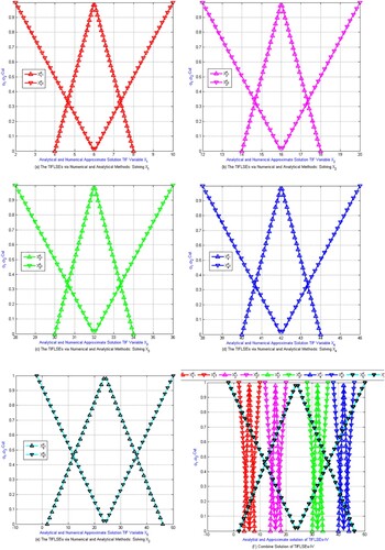
Table 4. Residual error comparison of semi-analytical and numerical schemes for solving TIFLSEs-III.

Parameter	BHMPM	GSM	JCM	ADMM	SORM
CPU-time	0.011	1.132	1.665	1.232	2.1615
NS	04.0	25.0	25.0	20.0	14.0
ERR	1.7E-030	3.5E-008	4.30E-005	0.15E-0018	4.13E-0013

The exact solution of TIFLSEs-IV with parameter σ₁σ₂ is given as: $\begin{array}{rl}{X}_1& =[x_1{]}_{({\sigma }_1,{\sigma }_2)}=〈\left[x_1^{L_1},x_1^{U_1}\right],\left[x_1^L,x_1^U\right]〉=〈\left[4+2{\sigma }_1,8-2{\sigma }_1\right],\left[6-4{\sigma }_2,6+4{\sigma }_2\right]〉\\ X_2& =[x_2{]}_{({\sigma }_1,{\sigma }_2)}\\ & =〈\left[x_2^{L_1},x_2^{U_1}\right],\left[x_2^L,x_2^U\right]〉=〈\left[14+2{\sigma }_1,18-2{\sigma }_1\right],\left[16-4{\sigma }_2,16+4{\sigma }_2\right]〉\\ X_3& =[x_3{]}_{({\sigma }_1,{\sigma }_2)}\\ & =〈\left[x_3^{L_1},x_3^{U_1}\right],\left[x_3^L,x_3^U\right]〉=〈\left[30+2{\sigma }_1,34-2{\sigma }_1\right],\left[32-4{\sigma }_2,32+4{\sigma }_2\right]〉\\ X_4& =[x_4{]}_{({\sigma }_1,{\sigma }_2)}\\ & =〈\left[x_4^{L_1},x_4^{U_1}\right],\left[x_4^L,x_4^U\right]〉=〈\left[40+2{\sigma }_1,44-2{\sigma }_1\right],\left[42-4{\sigma }_2,42+4{\sigma }_2\right]〉\end{array}$and $\begin{array}{rl}{X}_5& =[x_5{]}_{({\sigma }_1,{\sigma }_2)}\\ & =〈\left[x_5^{L_1},x_5^{U_1}\right],\left[x_5^L,x_5^U\right]〉=〈\left[2+22{\sigma }_1,46-22{\sigma }_1\right],\left[24-26{\sigma }_2,24+26{\sigma }_2\right]〉\end{array}$We apply HPM by taking as: $\begin{array}{rl}\stackrel{`}{\text{U}}& =\left(\begin{array}{cccccccccc}\text{0}& \text{5}& \text{7}& \text{8}& \text{9}& \text{3}& \text{0}& \text{0}& \text{0}& \text{0}\\ \text{4}& \text{5}& \text{3}& \text{7}& \text{0}& \text{0}& \text{0}& \text{0}& \text{0}& \text{1}\\ \text{1}& \text{0}& \text{3}& \text{4}& \text{5}& \text{0}& \text{2}& \text{0}& \text{0}& \text{0}\\ \text{9}& \text{8}& \text{7}& \text{6}& \text{5}& \text{0}& \text{0}& \text{0}& \text{0}& \text{0}\\ \text{2}& \text{3}& \text{7}& \text{0}& \text{1}& \text{0}& \text{0}& \text{0}& \text{1}& \text{0}\\ \text{3}& \text{0}& \text{0}& \text{0}& \text{0}& \text{0}& \text{5}& \text{7}& \text{8}& \text{9}\\ \text{0}& \text{0}& \text{0}& \text{0}& \text{1}& \text{4}& \text{5}& \text{3}& \text{7}& \text{0}\\ \text{0}& \text{2}& \text{0}& \text{0}& \text{0}& \text{1}& \text{0}& \text{3}& \text{4}& \text{5}\\ \text{0}& \text{0}& \text{0}& \text{0}& \text{0}& \text{9}& \text{8}& \text{7}& \text{6}& \text{5}\\ \text{0}& \text{0}& \text{0}& \text{1}& \text{0}& \text{2}& \text{3}& \text{7}& \text{0}& \text{1}\end{array}\right)\text{,}\\ \text{Y}{}_{{\sigma }_1}& =\left(\begin{array}{c}642+232{\sigma }_1\\ 502+16{\sigma }_1\\ 300+122{\sigma }_1\\ 608+170{\sigma }_1\\ 306+44{\sigma }_1\\ 1106-232{\sigma }_1\\ 534-16{\sigma }_1\\ 544-122{\sigma }_1\\ 948-170{\sigma }_1\\ 394-44{\sigma }_1\end{array}\right),\\ \text{Y}{}_{{\sigma }_2}& =\left(\begin{array}{c}874-302{\sigma }_2\\ 518-50{\sigma }_2\\ 422-154{\sigma }_2\\ 778-250{\sigma }_2\\ 350-70{\sigma }_2\\ 874+302{\sigma }_2\\ 518+50{\sigma }_2\\ 422+154{\sigma }_2\\ 778+250{\sigma }_2\\ 350+70{\sigma }_2\end{array}\right),\end{array}$ $\begin{array}{rl}\hat{\mathrm{G}}{}_{\sigma }& =\left(\begin{array}{cccccccccc}-3& 5& 7& 8& 9& 0& 0& 0& 0& 0\\ 4& 5& 3& 7& -1& 0& 0& 0& 0& 0\\ 1& -2& 3& 4& 5& 0& 0& 0& 0& 0\\ 9& 8& 7& 6& 5& 0& 0& 0& 0& 0\\ 2& 3& 7& -1& 1& 0& 0& 0& 0& 0\\ 0& 0& 0& 0& 0& -3& 5& 7& 8& 9\\ 0& 0& 0& 0& 0& 4& 5& 3& 7& -1\\ 0& 0& 0& 0& 0& 1& -2& 3& 4& 5\\ 0& 0& 0& 0& 0& 9& 8& 7& 6& 5\\ 0& 0& 0& 0& 0& 2& 3& 7& -1& 1\end{array}\right),\\ \\ \\ E_0^L& =\left(\begin{array}{c}2.020461245+2.0\ast {\sigma }_1\\ -1.094850009+2.0\ast {\sigma }_1\\ 51.85919889+2.0\ast {\sigma }_1\\ 47.67400728+2.0\ast {\sigma }_1\\ -10.09675741+22.0\ast {\sigma }_1\\ 6.020461245-2.0\ast {\sigma }_1\\ 2.905149991-2.0\ast {\sigma }_1\\ 55.85919889-2.0\ast {\sigma }_1\\ 51.67400728-2.0\ast {\sigma }_1\\ 33.90324259-22.0\ast {\sigma }_1\end{array}\right),E_0^U=\left(\begin{array}{c}4.020461245-4.0\ast {\sigma }_2\\ .9051499913-4.0\ast {\sigma }_2\\ 53.85919889-4.0\ast {\sigma }_2\\ \mathrm{.49.67400728}-4.0\ast {\sigma }_2\\ 11.90324259-26.0\ast {\sigma }_2\\ 4.020461245+4.0\ast {\sigma }_2\\ .9051499913+4.0\ast {\sigma }_2\\ 53.85919889+4.0\ast {\sigma }_2\\ 49.67400728+4.0\ast {\sigma }_2\\ 11.90324259+26.0\ast {\sigma }_2\end{array}\right),\end{array}$Approximate solution of the TIFLSEs-IV obtained by HAM after four iterations is $X_{{\sigma }_1}=\left(\begin{array}{c}3.9282+2.0\ast {\sigma }_1\\ 14.6399+2.0\ast {\sigma }_1\\ 30.289+2.0\ast {\sigma }_1\\ 40.678+2.0\ast {\sigma }_1\\ 2.487+22.0\ast {\sigma }_1\\ 8.928-2.0\ast {\sigma }_1\\ 18.640-2.0\ast {\sigma }_1\\ 30.289-2.0\ast {\sigma }_1\\ 40.678-2.0\ast {\sigma }_1\\ 45.487-22.0\ast {\sigma }_1\end{array}\right),X_{\sigma 2}=\left(\begin{array}{c}8.1282-4.0\ast {\sigma }_2\\ 17.640-4.0\ast {\sigma }_2\\ 32.289-4.0\ast {\sigma }_2\\ 42.678-4.0\ast {\sigma }_2\\ 23.487-26.0{\sigma }_2\\ 5.9282+4.0{\sigma }_2\\ 15.940+4.0{\sigma }_2\\ 32.289+4.0{\sigma }_2\\ 43.678+4.0\ast {\sigma }_2\\ 23.987+26.0\ast {\sigma }_2\end{array}\right).$The desired accuracy of the solutions with $\in ={10}^{-5}$ is acquired after 28 iterations and 1.737s and 1.432s computational CPU-time in the JCM and GSM methods, however in the BHMPM method, we obtain an estimated solution up to 25 decimal places i.e. $\in ={10}^{-25}$ after four iterations and 0.012s computational CPU-time. The exact solution of the TFLSEs-IV without ${\sigma }_{1,}{\sigma }_2-\mathrm{Cut}$ is given as: $\begin{array}{rl}{\xi }_{{\ddot{e}}_m}^{\ast }\left(x_1\right)& =\{\begin{array}{cc}{\displaystyle \frac{x-4}{2}}& \text{if }4<x<6,\\ 1& \text{if }x\in [6,6],\\ {\displaystyle \frac{x-8}{-2}}& 6<x<8,\\ 0& \text{otherwise}.\end{array},\\ {\xi }_{{\ddot{e}}_n}\left(x_1\right)& =\{\begin{array}{cc}{\displaystyle \frac{x-6}{-4}}& \text{if }2<x<6,\\ 1& \text{if }x\in [6,6],\\ {\displaystyle \frac{x-6}{4}}& 6<x<10,\\ 0& \text{otherwise}.\end{array},\\ {\xi }_{{\ddot{e}}_m}^{\ast }\left(x_2\right)& =\{\begin{array}{cc}{\displaystyle \frac{x-14}{2}}& \text{if }14<x<16,\\ 1& \text{if }x\in [16,16],\\ {\displaystyle \frac{x-18}{-2}}& 16<x<18,\\ 0& \text{otherwise}.\end{array},\\ {\xi }_{{\ddot{e}}_n}\left(x_2\right)& =\{\begin{array}{cc}{\displaystyle \frac{x-16}{-4}}& \text{if 1}2<x<16,\\ 1& \text{if }x\in [16,16],\\ {\displaystyle \frac{x-16}{4}}& 16<x<20,\\ 0& \text{otherwise}.\end{array},\\ {\xi }_{{\ddot{e}}_m}^{\ast }\left(x_3\right)& =\{\begin{array}{cc}{\displaystyle \frac{x-30}{2}}& \text{if }30<x<32,\\ 1& \text{if }x\in [32,32],\\ {\displaystyle \frac{x-34}{-2}}& 32<x<34,\\ 0& \text{otherwise}.\end{array},\end{array}$ $\begin{array}{rl}{\xi }_{{\ddot{e}}_n}\left(x_3\right)& =\{\begin{array}{cc}{\displaystyle \frac{x-32}{-4}}& \text{if }28<x<32,\\ 1& \text{if }x\in [32,32],\\ {\displaystyle \frac{x-32}{4}}& 32<x<36,\\ 0& \text{otherwise}.\end{array},\\ {\xi }_{{\ddot{e}}_m}^{\ast }\left(x_4\right)& =\{\begin{array}{cc}{\displaystyle \frac{x-40}{2}}& \text{if }20<x<25,\\ 1& \text{if }x\in [25,25],\\ {\displaystyle \frac{x-44}{-2}}& 25<x<30,\\ 0& \text{otherwise}.\end{array},\\ {\xi }_{{\ddot{e}}_n}\left(x_4\right)& =\{\begin{array}{cc}{\displaystyle \frac{x-42}{-4}}& \text{if }38<x<42,\\ 1& \text{if }x\in [42,42],\\ {\displaystyle \frac{x-42}{4}}& 42<x<46,\\ 0& \text{otherwise}.\end{array},\\ {\xi }_{{\ddot{e}}_m}^{\ast }\left(x_5\right)& =\{\begin{array}{cc}{\displaystyle \frac{x-2}{22}}& \text{if }2<x<24,\\ 1& \text{if }x\in [24,24],\\ {\displaystyle \frac{x-46}{-22}}& 24<x<46,\\ 0& \text{otherwise}\text{.}\end{array},\\ {\xi }_{{\ddot{e}}_n}\left(x_5\right)& =\{\begin{array}{cc}{\displaystyle \frac{x-24}{-26}}& \text{if - }2<x<24,\\ 1& \text{if }x\in [24,24],\\ {\displaystyle \frac{x-24}{26}}& 24<x<50,\\ 0& \text{otherwise}.\end{array}.\end{array}$Table 5 compares numerically the computational time seconds (CPU-time), number of iterations (NS), and residual error (ERR) of BHMPM, GSM, JCM, ADMM and SORM for solving TIFLSEs-IV. We can conclude from Table 4 that the BHMPM has better convergence behaviour and is more stable than the GSM and JCM technique.

5. Results and discussion

• In comparison to GSM, JCM, ADMM, and SORM, BHMPM is found to converge much faster and to be more efficient for solving TIFLSEs.

• The BHMPM method's primary benefit is that it can resolve all varieties of fuzzy TIFLSEs.

• A practical benefit of the BHMPM is that it lowers computation costs while keeping enhanced numerical solution accuracy.

• A large class system of TIFLSEs can be efficiently, quickly, and correctly solved by BHMPM using closed form solutions that quickly converge to exact solutions.

• The BHMPM has been shown to be quite effective and produces large accuracy reductions, calculation time savings, and accuracy significantly, as shown in Figures 2–5 and Tables 1–4.

Table 5. Residual error comparison of semi-analytical and numerical schemes for solving TIFLSEs-IV.

Parameter	BHMPM	GSM	JCM	ADMM	SORM
CPU-time	0.012	1.432	1.737	1.732	2.737
NS	04.0	24.0	28.0	15.0	21.0
ERR	4.8E-035	6.7E-005	8.3E-003	0.74E-0015	0.13E-003

6. Conclusion

In this research, BHMPM was used to solve a $n\times n$ triangular intuitionistic fuzzy linear systems of equations with $2n\times 2n$ crisp coefficients, an unknown triangular intuitionistic fuzzy variable, and the right hand side vector as intuitionistic fuzzy numbers. The BHMPM was found to be efficient and practical since it only requires the non-singularity of the coefficient matrix of TIFLS while the Jacobi and Gauss-Seidel methods required either a dominating diagonal value or non-zero diagonal entries in the coefficient matrix. By comparing approximate results with exact solution, we have shown this method to be more reliable. Numerical examples demonstrate that the BHMPM is an effective method for resolving triangular intuitionistic fuzzy linear problems. Also, BHMPM outperforms, Adomins decomposition method, Successive Over-Relaxation method, block Jacobi and Gauss-Seidel methods in terms of the number of iterations, computational time in second (CPU-time) and the Haussdorff distance. Therefore, the future studies will focus on solving generalized TIFLSEs, and its application in a generalized intuitionistic fuzzy environment.

Authors’ contributions

All authors’ contribute equally in the preparation of this manuscript.

Disclosure statement

No potential conflict of interest was reported by the author(s).

Data availability statement

No data were used to support this study.

References

- Biswas A, Roy SK, Mondal SP, et al. Evolutionary algorithm based approach for solving transportation problems in normal and pandemic scenario. Appl Soft Comput. 2022;129:109576. doi:10.1016/j.asoc.2022.109576
- Rahaman M, Abdulaal OA, Bafail M, et al. An insight into the impacts of memory, selling price and displayed stock on a retailer's decision in an inventory management problem. Fractal Fractional. 2022;6(9):531. doi:10.3390/fractalfract6090531
- Rahaman M, Mondal SP, Alam S, et al. Study of a fuzzy production inventory model with deterioration under Marxian principle. Int J Fuzzy Syst. 2022;24(4):2092–2106. doi:10.1007/s40815-021-01245-0
- Rahaman M, Mondal SP, Chatterjee SP, et al. Generalization of classical fuzzy economic order quantity model based on memory dependency via fuzzy fractional differential equation approach. J Uncert Syst. 2022;15(01):2250003. doi:10.1142/S1752890922500039
- Rahaman M, Mondal SP, Chatterjee B, et al. Application of fractional calculus on the crisp and uncertain inventory control problem. In: Handbook of research on advances and applications of fuzzy sets and logic. IGI Global. p. 120–148
- Zadeh LA. Fuzzy sets. Inf Control. Jan 1965;8:338–353. doi:10.1016/S0019-9958(65)90241-X
- Zadeh LA. The concept of a linguistic variable and its application to approximation reasoning. Inform Sci. Jan 1975;3:199–249. doi:10.1016/0020-0255(75)90036-5
- Chang SSL, Zadeh LA. On fuzzy mapping and control. IEEE T Syst Man Cy B. Jan 1972;2:30–34. doi:10.1109/TSMC.1972.5408553
- Dubois D, Prade H. Operations on fuzzy numbers. Int J Sys Sci. Jan 1978;9(6):613–626. doi:10.1080/00207727808941724
- Mizumoto M. Some properties of fuzzy numbers. Inf Control. Aug 1976;31(4):312–340. doi:10.1016/S0019-9958(76)80011-3
- Mizumoto M, Tanaka K. The four operations of arithmetic on fuzzy numbers. Syst Comput Cont. Feb 1976;7(5):73–81.
- Nahmias S. Fuzzy variables. Fuzzy Set Syst. Apr 1978;12(2):97–111. doi:10.1016/0165-0114(78)90011-8
- Zimmermann HJ. Fuzzy sets theory and its application. Dordrecht: Kluwer Academic Press; 1991.
- Friedman M, Ma M, Kandel A. Fuzzy linear systems. Fuzzy Set Syst. Jun 1998;96(2):201–209. doi:10.1016/S0165-0114(96)00270-9
- Abbasbandy S, Jafarian A, Ezzati R. Conjugate gradient method for fuzzy symmetric positive definite system of linear equations. Appl Math Comput 2005;171(2):1184–1191.
- Amirfakhrian M. Numerical solution of a fuzzy system of linear equations with polynomial parametric form. Int J Comput Math. Jul 2007;84(7):1089–1097. doi:10.1080/00207160701294400
- Chakraverty S, Behera D. Fuzzy system of linear equations with crisp coefficients. J Intell Fuzzy Syst. Jan 2013;25(1):201–207. doi:10.3233/IFS-2012-0627
- Behera D, Chakraverty S. Solving fuzzy complex system of linear equations. Inform Sci. Sep 2014;277(1):154–162. doi:10.1016/j.ins.2014.02.014
- Abbasbandy S, Jafarian A. Steepest descent method for system of fuzzy linear equations. Appl Math Comput. Apr 2006;175(1):823–833.
- Kargar R, Allahviranloo T, Rostami-Malkhalifeh M, et al. A proposed method for solving fuzzy system of linear equations. Sci World J. Jan 2014;2014:1–10. doi:10.1155/2014/782093
- Farahani H, Nehi HM, Paripour M. Solving fuzzy complex system of linear equations using eigenvalue method. J Intell Fuzzy Syst. Jan 2016;31(3):1689–1699. doi:10.3233/JIFS-152046
- Salahuddin S. Iterative algorithms for a fuzzy system of random nonlinear equations in Hilbert spaces. Commun Korean Math Soc. Feb 2017;32(2):333–352. doi:10.4134/CKMS.c160088
- Koam AN, Akram M, Muhammad G, et al. LU decomposition scheme for solving-polar fuzzy system of linear equations. Math Probl Eng. Sep 2020;2020:1–10.
- Buckley JJ, Qu Y. On using a-cuts to evaluate equations. Fuzzy Set Syst. Dec 1990;38(3):309–312. doi:10.1016/0165-0114(90)90204-J
- Buckley JJ, Qu Y. Solving fuzzy equations: a new solution concept. Fuzzy Set Syst. Feb 1991;39(3):291–301. doi:10.1016/0165-0114(91)90099-C
- Allahviranloo T, Asari S. Numerical solution of fuzzy polynomial by Newton-Raphson method. J Appl Math. Jan 2011;2011:17–23.
- Cho YJ, Huang NJ, Kang SM. Nonlinear equations for fuzzy mapping in probabilistic normed spaces. Fuzzy Set Syst. Feb 2000;110(1):115–122. doi:10.1016/S0165-0114(98)00009-8
- Dennis JE, Schnabel RB. Numerical methods for unconstrained optimization and nonlinear equations. New Jersey: Prentice-Hall; 1983.
- Sulaiman IM, Mamat M, Waziri MY, et al. Solving fuzzy nonlinear equation via Levenberg-Marquardt method. Far East J Math Sci. 2018;103(1):1547–1558.
- Ma J, Feng G. An approach to H1 control of fuzzy dynamic systems. Fuzzy Set Syst. Aug 2003;137(1):367–386. doi:10.1016/S0165-0114(02)00281-6
- Mosleh M. Solution of dual fuzzy polynomial equations by modified Adomian decomposition method. Fuzzy Inform Eng. March 2013;5(1):45–56. doi:10.1007/s12543-013-0132-6
- Nehi HM. A new ranking method for intuitionistic fuzzy numbers. Int J Fuzzy Syst. Mar 2010;1(1):80–86.
- Elizabeth S, Sujatha L. Project scheduling method using triangular intuitionistic fuzzy numbers and triangular fuzzy numbers. Appl Math Sci. Jan 2015;9(1-4):185–198.
- Akram M, Muhammad G, Allahviranloo T, et al. LU decomposition method to solve bipolar fuzzy linear systems. J Intell Fuzzy Syst. Jan 2020;39(3):3329–3349. doi:10.3233/JIFS-201187
- Akram M, Ali M, Allahviranloo T. Certain methods to solve bipolar fuzzy linear system of equations. Comput Appl Math Sep 2020;39(3):1–28.
- Akram M, Allahviranloo T, Pedrycz W, et al. Methods for solving LR-bipolar fuzzy linear systems. Soft comput Jan 2021;25(1):85–108. doi:10.1007/s00500-020-05460-z
- Akram M, Ali M, Allahviranloo T. A method for solving bipolar fuzzy complex linear systems with real and complex coefficients. Soft comput. Mar 2022;5(26):2157–2178. doi:10.1007/s00500-021-06672-7
- Jafari R, Yu W. Uncertainty nonlinear systems modeling with fuzzy equations. IEEE Int Conf Inf Reuse Integr. Aug 2015;13:182–188.
- Jafari R, Razvarz S, Gegov A. A new computational method for solving fully fuzzy nonlinear systems. In International Conference on Computational Collective Intelligence. Cham: Springer; Sep 2018. p. 503–612.
- Jafari R, Razvarz S, Gegov A, et al. Fuzzy control of uncertain nonlinear systems with numerical techniques: a survey. In UK Workshop on Computational Intelligence. Cham: Springer; Sep. 2019. p. 3–14.
- Jafari R, Razvarz S, Gegov A. A novel technique for solving fully fuzzy nonlinear systems based on neural networks. Vietnam J Comput Sci. 2020;1(7):93–107. doi:10.1142/S2196888820500050
- He JH. Homotopy perturbation technique. Comput Method Appl Mech Eng. Aug 1999;178(3–4):257–262. doi:10.1016/S0045-7825(99)00018-3
- Noeiaghdam S, Araghi MAF, Sidorov D. Dynamical strategy on homotopy perturbation method for solving second kind integral equations using the CESTAC method. J Comput Appl Math. 2022;411:114226. doi:10.1016/j.cam.2022.114226
- Noeiaghdam S, Dreglea A, He J, … Sidorov N. Error estimation of the homotopy perturbation method to solve second kind Volterra integral equations with piecewise smooth kernels: application of the CADNA library. Symmetry. 1730;12(10):2022.
- Najafi HS, Edalatpanah SA. Homotopy perturbation method for linear programming problems. Appl Math Mod. Mar 2014;38(5-6):1607–1611. doi:10.1016/j.apm.2013.09.011
- Edalatpanah SA, Rashidi MM. On the application of homotopy perturbation method for solving systems of linear equations. Int Schol Res Notice. 2014: 1–5.
- Najafi HS, Edalatpanah SA, Vosoughi N. A discussion on the practicability of an analytical method for solving system of linear equations. Am J Num Anal. Jan 2014;2(3):76–78.
- Najafi HS, Edalatpanah SA, Refahisheikhani AH. An analytical method as a preconditioning modeling for systems of linear equations. Comput Appl Math. Jan 2018;37(2):922–931. doi:10.1007/s40314-016-0376-y
- Najafi HS, Edalatpanah SA, Sheikhani AR. Application of homotopy perturbation method for fuzzy linear systems and comparison with Adomian’s decomposition method. Chinese J Math. Feb 2013;2013:1–7. doi:10.1155/2013/584240
- Miao SX. Block homotopy perturbation method for solving fuzzy linear systems. World Acad Sci Eng Technol. Mar 2011;51(3):1062–1065.
- Najafi HS, Edalatpanah SA. On the application of Liaos method for solving linear systems. Ain Shams Eng J. Sep 2013;4(3):501–505. doi:10.1016/j.asej.2012.10.004
- Edalatpanah SA. Systems of neutrosophic linear equations. Neutrosophic Sets Syst. May 2020;33(1):92–104.
- Najafi HS, Edalatpanah SA. An improved model for iterative algorithms in fuzzy linear systems. Comput Math Model Jul 2013;24(3):443–451. doi:10.1007/s10598-013-9189-7
- Najafi HS, Edalatpanah SA. H-matrices in fuzzy linear systems. Int J Comput Math. Jan 2014;13:1–10. doi:10.1155/2014/394135
- Mahapatra GS, Roy TK. Reliability evaluation using triangular intuitionistic fuzzy numbers arithmetic operations. World Acad Sci Eng Technol Feb 2009;50(1):574–581.
- Li DF, Nan JX, Zhang MJ. A ranking method of triangular intuitionistic fuzzy numbers and application to decision making. Int J Comput Intell Syst. Oct 2010;3(5):522–530.
- Seikh MR, Nayak PK, Pal M. Notes on triangular intuitionistic fuzzy numbers. Int J Math Oper. Jan 2013;5(4):446–465. doi:10.1504/IJMOR.2013.054730
- Shams M, Kausar N, Khan N, et al. Modified block homotopy perturbation method for solving triangular linear diophantine fuzzy system of equations. Adv Mech Eng. 2023;15(3):16878132231159519. doi:10.1177/16878132231159519
- Kumar A, Babbar N, Bansal A. A new approach for solving fully fuzzy linear systems. Adv Fuzzy Syst. 2011;2011:1–8. doi:10.1155/2011/943161
- Allahviranloo T, Salahshour S. Fuzzy symmetric solutions of fuzzy linear systems. J Comput Appl Math. 2011;235(16):4545–4553. doi:10.1016/j.cam.2010.02.042
- Ezzati R, Khezerloo S, Yousefzadeh A. Solving fully fuzzy linear system of equations in general form. J Fuzzy Set Val Anal. 2012;2012:1–11. doi:10.5899/2012/jfsva-00117
- Behera D, Chakraverty S. Fuzzy centre based solution of fuzzy complexlinear system of equations. Int J Uncertain Fuzziness Knowl-Based Syst. 2013;21(04):629–642. doi:10.1142/S021848851350030X
- Lodwick WA, Dubois D. Interval linear systems as a necessary step in fuzzy linear systems. Fuzzy Sets Syst. 2015;281:227–251. doi:10.1016/j.fss.2015.03.018
- Akram M, Saleem D, Allahviranloo T. Linear system of equations in m-polar fuzzy environment. J Intell Fuzzy Syst. 2019;37(6):8251–8266. doi:10.3233/JIFS-190744
- Mikaeilvand N, Noeiaghdam Z, Noeiaghdam S, et al. A novel technique to solve the fuzzy system of equations. Mathematics. 2020;8(5):850. doi:10.3390/math8050850
- Saqib M, Akram M, Bashir S. Certain efficient iterative methods for bipolar fuzzy system of linear equations. J Intell Fuzzy Syst. 2020;39(3):3971–3985. doi:10.3233/JIFS-200084
- Akram M, Allahviranloo T, Pedrycz W, et al. Methods for solving LR-bipolar fuzzy linear systems. Soft comput. 2021;25(1):85–108. doi:10.1007/s00500-020-05460-z
- Goetschel R, Voxman W. Elementary calculus. Fuzzy Set Syst. Apr 1986;18:31–43. doi:10.1016/0165-0114(86)90026-6
- Mitchell HB. Ranking-intuitionistic fuzzy numbers. Int J Uncert Fuzz Knowl-Based Syst. Jan 2004;12(3):377–386. doi:10.1142/S0218488504002886
- Abbasbandy S, Asady B. Newton's method for solving fuzzy non-linear equations. Appl Math Comput. Dec 2004;159(2):349–356.
- Shaw andT AK, Roy K. Some arithmetic operations on triangular intuitionistic fuzzy number and its application on reliability evaluation. Int J Fuzzy Math Syst. Jan 2012;2(4):363–382.
- Friedman M, Ming M, Kandel A. Fuzzy linear systems. Fuzzy Set Syst. Jan 1998;96(2):201–209. doi:10.1016/S0165-0114(96)00270-9
- Miao SX, Zheng B, Wang K. Block SOR methods for fuzzy linear systems. J Appl Math Comput. Feb 2008;26(1):201–218. doi:10.1007/s12190-007-0019-y
- Buckley JJ, Qu Y. Solving systems of linear fuzzy equations. Fuzzy Set Syst. Sep 1990;43(1):33–43. doi:10.1016/0165-0114(91)90019-M
- Banerjee S, Roy TK. Arithmetic operations on generalized trapezoidal fuzzy number and its applications. Turkish J Fuzzy Syst. Jan 2012;3(1):16–44.
- Dubois D, Prade H. Fuzzy sets and systems: theory and application. New York: Academic Press; 1980.
- Allahviranloo T. Numerical methods for fuzzy system of linear equations. Appl Math Comput. Aug 2004;155(2):493–502.
- Burden RL, Faires JD. Numerical methods for fuzzy system of linear equations. Boston (MA): Belmont Thomson, Brooks/Cole Press; 2005. p. 1–863.