Computational analysis of corruption dynamics insight into fractional structures

Abstract

The fractional derivative that is used to compute the solution of the corruption system with Power-Law Kernel, Mittag-Leffler Kernel, and Exponential Decay Kernel. It is important to study and analyse corruption dynamics, because it is an act that has a direct effect on public rights, and because of this the right of the rightful owner, just got destroyed. Using hypothesis theory for differential equation, this work suggests and assesses a nonlinear deterministic model for the dynamics of corruption. Positivity and boundedness are verified for the proposed corruption model to identify the level of resolution of corruption factor in society. Fractional-order corruption model is investigated with different kernels for efficient results. The necessary criteria for the best control of corruption transmission were identified using Pontryagin's maximal concept. The numerical simulation showed that corruption must be resisted by an integrated control strategy. Numerical simulations are used to demonstrate the correctness of the proposed approaches. Finally, simulations are derived for the proposed schemes to check the effectiveness of the results and to analyse the corruption behaviour in society as well as dynamically highlight the propagation of corruption group.

KEYWORDS:

• Algorithm’s
• fractional structure
• Pontryagin’s maximal
• simulation

MATHEMATICS SUBJECT CLASSIFICATIONS:

• SC: 68V20
• 68V30
• 68V25
• 65-11

1. Introduction

In order to obtain unlawful power for personal interests and illegal profit, the criminal offence or dishonest performed by a single person or an organization is termed corruption. Corruption may be done over a wide span including fraud, illegal payments, bribery and many other unlawful means. Corruption in the political sector occurs when an office bearer or another public servant performs a legitimate service to his advantage. Corruption is very common in our country.

Corruption and crime are social ills that are commonplace in almost every country around the world in varying degrees and proportions. Every nation designed some structures and allocated resources to eliminate or reduce corruption to a maximum extent. Policies and rules have been defined to deal with it and they fall under the anti-corruption section.

Corruption is basically an unlawful activity for personal gain, through the abuse of power or authority by officials from the public sector (government) or the private sector (corporation) [1]. Cuervo-Cazurra et al. examine worldwide commercial corruption, offering a critical appraisal of the problem and recommendations for future research. Because of its illegal nature, variances in perceptions of illegality, and heterogeneity in the application of anti-bribery laws between countries, I believe that corruption serves as a laboratory for developing international business studies in [2]. The facts and ideas offered by top researchers globally provide a backdrop for supplemental and supplementary probes and theories, according to G Geis et al. [3], widespread corruption, and lawlessness [4]. Corruption may be originated on either the demand or supply side [5]. The rules of democracy, law and human rights are all threatened by corruption and integrity. Economic development is hampered by inequity and social fairness and puts the market economy at risk for its proper functioning and impartiality [2, 6]. It is a major concern in every country on the planet, particularly in emerging nations [6]. Although the majority of countries have policies or strategies in place to combat corruption, it is still a public epidemic.

Statistical models with comprehensive and detailed control analysis are some key tools in determining and understanding corruption fluctuations and when it comes to corruption decision-making. In the present study, some research studies on corruption exist. A study by [7] suggested and analysed the determining model of human corruption. They calculated the basic reproduction number (BRN), the non-corruption rating scale, and the inherent balance that point to the results of numerical simulations that indicated that corruption can be managed to some extent but not removed. The authors designed and analysed a model by using mathematical tools of the power of corruption [2]. The basic production number and equity points that are free of corruption and corruption are determined. Lemecha [8] elevated them by considering the statistical model of corruption and also the awareness initiated by anti-corruption and prison counselling. The introduction of the unique points free from corruption and endless equality was analysed, and a fundamental production number was computerized. Research in [9] has introduced triangular models that represent the laws of increasing trend or decreasing trend of corruption. In [6], a mathematical model was developed independently to define the corruption level. The research work [10] considered the Game’s theoretical methodology to deal with corruption. Khan [11] developed the anti-corruption model and presented that it is possible to eliminate corruption if the ratio of the rate of dismissal to the level of corruption is equal to unity. The authors [12] created a SIR model for the power of corruption. In addition, the study has expanded the procedure to analyse complete control with one correct control policy. The term corruption, according to KO Jackob, refers to the practice of abusing a public trust or office for personal gain. When there is no political resolve to tackle corruption, it poses a threat to national development and prosperity. EACC’s anti-corruption tactics include prevention and disengagement activities [13].

Some respectable authors, on the one hand, lauded these beginning conditions for their ability to account for aberrant processes. Caputo, on the other hand, proposed an alternative differential operator based on experimental evidence, which is the convolution of a function’s derivative with a power law. The normal initial condition is obtained by applying the Laplace transform to this variant. Furthermore, the function was assumed to be differentiable, which, some writers thought, was a constraint in theory but was a good differentiation in fact, which was necessary for evaluating modifications [14]. With a non-local and no-singular kernel, we presented a novel fractional derivative. We demonstrated some of the new derivative’s valuable qualities and used them to solve the fractional heat transfer model [15] and they do not meet several typical derivative properties such as the index law. We offer a numerical approach and mathematical analysis for the well-known three-dimensional quadratic autonomous self-govern system, which is chaotic due to the coexistence of multi-scroll attractors, as shown by M Khumalo et al. In the Caputo sense, the scheme is based on the Atangana-Baleanu fractional derivative. The fractional derivatives are introduced to the non-local and non-singular kernel in the formulation of these schemes. After that, the fractional derivative is approximated using the Adams–Bashforth scheme family [16, 17]. The study concludes that foreign aid does not result in encouraging and significant changes in overall economic growth in developing economies. By contrast, corruption has a powerful impact on foreign aid effectiveness [19].

Different authors use fractional derivatives to understand the actual behaviour of the different types of dynamics. Accordingly, a relatively novel numerical treatment is introduced to investigate and interpret approximate solutions to telegraph and Cattaneo models of time-fractional derivatives in the Caputo sense [20, 21]. The reliability, stability and exactness of the proposed FF-ANN-PSO-IPM are established through comparison with outcomes of the standard numerical procedure with the Adams method for both single and multiple autonomous trials with precision of order 4 to 8 decimal places of accuracy [22]. The authors present the analytical treatment to the bioheat transfer Pennes model by modern fractional derivatives and their related phenomena in [23–26]. Some authors consider an initial-value problem comprising this generalization and analyse the existence and the uniqueness of its solution for different epidemic and non-epidemic phenomena, also see their behaviours in [27–31]. A computational method, based on B-spline polynomials and their operational matrix of Atangana-Baleanu fractional integration, is proposed for the numerical solution of this class of problems [32]. For more details, see [37–42].

In this work, we propose a dynamic of corruption with a fractional operator in the introduction section and preliminaries are given to understand the corruption dynamics and methodology used to analyse, respectively. The qualitative and auantitative analysis of the system was also treated. The stability and uniqueness of the system are also presented by using fixed point theory results. Analysis of the model was made with (i) Mitting Lifter Kernel (ii) Power Law Kernel (iii) Exponential Decay Kernel. In the end, numerical simulations are made with the support of theoretical results.

2. Basic of fractional calculus

2.1. Definition: [18]

Allow f (t) to be a function that isn’t always differentiable. Consider the numbers $0<\alpha ,\beta \le 1$, where is the fractal dimension and is the fractional order. The following is a definition of a Fractal-Fractional derivative with order 0 and 1 and a Power-Law Kernel: (1) ${}_0^{\mathrm{FFP}}{D}_t^{\alpha ,\beta }f(t)=\frac{1}{\mathrm{\Gamma }(1-\alpha )}\frac{d}{d{t}^{\beta }}{\int }_0^{t}f(\tau ){(t-\tau )}^{-\alpha }\mathrm{d\tau }\text{where }C(t)=-(\mu +\mathrm{\pi \beta }+)C$(1) (2) $\frac{\mathrm{df}(t)}{d{t}^{\beta }}=\underset{t\to t_1}{\text{lim}}\frac{f(t)-f(t_1)}{t^{2-\beta }-t_1^{2-\beta }}(2-\beta )$(2)

2.2. Definition: [18]

The Exponential Decay Kernel for Fractal-Fractional Derivative is defined as (3) ${}_0^{\mathrm{FFE}}{D}_t^{\alpha ,\beta }f(t)=\frac{M(\alpha )}{1-\alpha }\frac{d}{d{t}^{\beta }}{\int }_0^{t}f(\tau )\text{exp}\left[-\frac{\alpha }{1-\alpha }(t-\tau )\right]\mathrm{d\tau }$(3)

2.3. Definition: [18]

The Mittag-Leffler Kernel for the Fractal-Fractional Derivative can be defined as (4) ${}_0^{\mathrm{FFM}}{D}_t^{\alpha ,\beta }f(t)=\frac{\mathrm{AB}(\alpha )}{1-\alpha }\frac{d}{d{t}^{\beta }}{\int }_0^{t}f(\tau )E_{\alpha }\left[-\frac{\alpha }{1-\alpha }{(t-\tau )}^{\alpha }\right]\mathrm{d\tau }$(4)

2.4. Definition: [18]

Power law-type kernel within the FFI with order $(\alpha ,\beta )$ is defined as (5) ${}_0^{\mathrm{FFP}}{I}_{0,t}^{\alpha ,\beta }f(t)=\frac{1}{\mathrm{\Gamma }(\alpha )}{\int }_0^t{(t-\tau )}^{\alpha -1}{\tau }^{1-\beta }f(\tau )\mathrm{d\tau }$(5)

2.5. Definition: [18]

The decay-type kernel within the FFI with order $(\alpha ,\beta )$ is defined as (6) ${}_0^{\mathrm{FFE}}{I}_{0,t}^{\alpha ,\beta }f(t)=\frac{\beta (1-\alpha )t^{\beta -1}f(t)}{\text{P}(\alpha )}+\frac{\mathrm{\alpha \beta }}{P(\alpha )}{\int }_0^t{\tau }^{\beta -1}f(\tau )\mathrm{d\tau }$(6)

2.6. Definition: [18]

The Mittag-Leffler-type kernel within the FFI with order $(\alpha ,\beta )$ is defined as (7) ${}_0^{\mathrm{FFM}}{I}_{0,t}^{\alpha ,\beta }f(t)=\frac{\beta (1-\alpha )t^{\beta -1}f(t)}{\mathrm{CB}(\alpha )}+\frac{\mathrm{\alpha \beta }}{\mathrm{CB}(\alpha )}{\int }_0^t(t-\tau ){\tau }^{\beta -1}f(\tau )\mathrm{d\tau }$(7)

3. Corruption model

At all times during the study, for all humans, we consider a positive natural death rate. Susceptible persons will be transferred to the exposed class if they have a rate of contact with corrupted people of rate p, with a p per contact likelihood of corruption transmission. Individuals moved at a pace to the contaminated compartment with the remainder travelling to the recovered compartments. Corrupted persons learn about the effect of their actions in prison and move to the recovered subpopulation at a rate of these rescued individuals were transferred at a rate of to the vulnerable groups, with the remaining percentage going to the honesty section. All parameter descriptions are listed in Table 1. Concerning the above considerations, the model will be controlled by the following system of differential equations: (8) $\begin{array}{rl}\frac{\mathrm{dS}}{\mathrm{dt}}& =\mathrm{\Pi }+(1-\theta )\mathrm{\epsilon R}-\mathrm{p\beta SC}-(k+\mu )S\\ \frac{\mathrm{dE}}{\mathrm{dt}}& =\mathrm{p\beta SC}-(\delta +\mu )E\\ \frac{\mathrm{dC}}{\mathrm{dt}}& =\mathrm{\alpha \delta E}-(\sigma +\mu )C\\ \frac{\mathrm{dR}}{\mathrm{dt}}& =\mathrm{\sigma C}+(1-\alpha )\mathrm{\delta E}-(\epsilon +\mu )R\\ \frac{\mathrm{dH}}{\mathrm{dt}}& =\mathrm{\kappa S}+\mathrm{\theta \epsilon R}-\mathrm{\mu H}\end{array}$(8) with the initial condition (9) $\{\text{S}(0)=S_0,\text{E}(0)=E_0,\text{C}(0)=C_0,\text{R}(0)=R_0,\text{H}(0)=H_0\}\ge 0$(9)

Table 1. Description of parameters of the corruption model.

Parameter	Description
$p$	Possibility of corruption transmission per contact
Β	Sensitive person to corrupt person contact rate
Δ	The rate at which exposed individuals become corrupted
Σ	The rate at which corrupt people recover
Ε	The rate at which those who recover become honest
$k$	The proportion of people who join the faithful Population from sensitive population
$\mu$	The death rate of all human beings
$\alpha$	The proportion of people who are involved in corruption. Sub-population from the exposed compartment
$\theta$	The proportion of people who join the faithful Sub-population from the exported compartment

3.1. Positive solutions with non-local operators

This section shows that solutions to a fractional calculus model with non-local operators are positive. With non-local operators, all solutions are positive if all beginning conditions are positive. To begin, we’ll look at the Caputo–Fabrizio case. (10) $\begin{array}{rl}S(t)\ge & S(0)\text{exp}\left[-\frac{\alpha (k+\mu +\mathrm{p\beta }\parallel C{\parallel }_{\mathrm{\infty }})t}{M(\alpha )-(1-\alpha )(k+\mu +\mathrm{p\beta }\parallel C{\parallel }_{\mathrm{\infty }})}\right]\mathrm{\forall t}\ge 0\\ E(t)\ge & E(0)\text{exp}\left[-\frac{\alpha (\delta +\mu )t}{M(\alpha )-(1-\alpha )(\delta +\mu )}\right]\mathrm{\forall t}\ge 0\\ C(t)\ge & C(0)\text{exp}\left[-\frac{\alpha (\sigma +\mu )t}{M(\alpha )-(1-\alpha )(\sigma +\mu )}\right]\mathrm{\forall t}\ge 0\\ R(t)\ge & R(0)\text{exp}\left[-\frac{\alpha (\epsilon +\mu )t}{M(\alpha )-(1-\alpha )(\epsilon +\mu )}\right]\mathrm{\forall t}\ge 0\\ H(t)\ge & H(0)\text{exp}\left[-\frac{\mathrm{\alpha \mu t}}{M(\alpha )-(1-\alpha )\mu }\right]\mathrm{\forall t}\ge 0\end{array}$(10)

With the Caputo derivative, we obtain (11) $\begin{array}{rl}S(t)\ge & S(0)E_{\alpha }[-(k+\mu +\mathrm{p\beta }\parallel C{\parallel }_{\mathrm{\infty }})t^{\alpha }]\mathrm{\forall t}\ge 0\\ E(t)\ge & E(0)E_{\alpha }[-(\delta +\mu )t^{\alpha }]\mathrm{\forall t}\ge 0\\ C(t)\ge & C(0)E_{\alpha }[-(\sigma +\mu )t^{\alpha }]\mathrm{\forall t}\ge 0\\ R(t)\ge & R(0)E_{\alpha }[-(\epsilon +\mu )t^{\alpha }]\mathrm{\forall t}\ge 0\\ H(t)\ge & H(0)E_{\alpha }[-\mu t^{\alpha }]\mathrm{\forall t}\ge 0\end{array}$(11) We obtain the Atangana-Baleanu derivative (12) $\begin{array}{rl}S(t)\ge & S(0)E_{\alpha }\left[-\frac{\alpha (k+\mu +\mathrm{p\beta }\parallel C{\parallel }_{\mathrm{\infty }})t^{\alpha }}{\mathrm{AB}(\alpha )-(1-\alpha )(k+\mu +\mathrm{p\beta }\parallel C{\parallel }_{\mathrm{\infty }})}\right]\mathrm{\forall t}\ge 0\\ E(t)\ge & E(0)E_{\alpha }\left[-\frac{\alpha (\delta +\mu )t^{\alpha }}{\mathrm{AB}(\alpha )-(1-\alpha )(\delta +\mu )}\right]\mathrm{\forall t}\ge 0\\ C(t)\ge & C(0)E_{\alpha }\left[-\frac{\alpha (\sigma +\mu )t^{\alpha }}{\mathrm{AB}(\alpha )-(1-\alpha )(\sigma +\mu )}\right]\mathrm{\forall t}\ge 0\\ R(t)\ge & R(0)E_{\alpha }\left[-\frac{\alpha (\epsilon +\mu )t^{\alpha }}{\mathrm{AB}(\alpha )-(1-\alpha )(\epsilon +\mu )}\right]\mathrm{\forall t}\ge 0\\ H(t)\ge & H(0)E_{\alpha }\left[-\frac{\mathrm{\alpha \mu }{t}^{\alpha }}{\mathrm{AB}(\alpha )-(1-\alpha )\mu }\right]\mathrm{\forall t}\ge 0\end{array}$(12)

Theorem 3.1:

Along the starting circumstances, the solution of the proposed corruption model given in system (8) is unique and bounded in $R_{+}^5$.

Proof:

We’ve obtained $\begin{array}{rl}{}_0^{\mathrm{FFE}}{D}_t^{\alpha ,\beta }S{|}_{S=0}& =\mathrm{\Pi }+(1-\theta )\mathrm{\epsilon R}\ge 0\\ {}_0^{\mathrm{FFE}}{D}_t^{\alpha ,\beta }E{|}_{E=0}& =\mathrm{p\beta SC}\ge 0\\ {}_0^{\mathrm{FFE}}{D}_t^{\alpha ,\beta }C{|}_{C=0}& =\mathrm{\alpha \delta E}\ge 0\\ {}_0^{\mathrm{FFE}}{D}_t^{\alpha ,\beta }R{|}_{R=0}& =\mathrm{\sigma C}+(1-\alpha )\mathrm{\delta E}\ge 0\\ {}_0^{\mathrm{FFE}}{D}_t^{\alpha ,\beta }H{|}_{H=0}& =\mathrm{\kappa S}+\mathrm{\theta \epsilon R}\ge 0\end{array}$If $\{S(0),E(0),C(0),R(0),H(0)\}\in R_{+}^5$, then it is impossible to exit the hyperplane, according to the answer. The domain $R_{+}^5$ is a positively invariant set since the vector field on each hyper-plane around the non-negative orthant likewise points to $R_{+}^5$ which shows a positive and bounded solution for the proposed system.

3.2. Application of corruption dynamic model

In this part, the proposed mathematical corruption dynamic model is subjected to the new differential and integral operators. The conventional differential operator will be replaced with the operator with Power-Law, Exponential Decay, and Mittag-Leffler Kernels. Additionally, the version with variable order will be applied. We start with an exponentially decaying kernel. (13) $\begin{array}{rl}{}_0^{\mathrm{FFE}}{D}_t^{\alpha ,\beta }S& =\mathrm{\Pi }+(1-\theta )\mathrm{\epsilon R}-\mathrm{p\beta SC}-(k+\mu )S\\ {}_0^{\mathrm{FFE}}{D}_t^{\alpha ,\beta }E& =\mathrm{p\beta SC}-(\delta +\mu )E\\ {}_0^{\mathrm{FFE}}{D}_t^{\alpha ,\beta }C& =\mathrm{\alpha \delta E}-(\sigma +\mu )C\\ {}_0^{\mathrm{FFE}}{D}_t^{\alpha ,\beta }R& =\mathrm{\sigma C}+(1-\alpha )\mathrm{\delta E}-(\epsilon +\mu )R\\ {}_0^{\mathrm{FFE}}{D}_t^{\alpha ,\beta }H& =\mathrm{\kappa S}+\mathrm{\theta \epsilon R}-\mathrm{\mu H}\end{array}$(13) For simplicity, we’ll express the equation as follows: (14) $\begin{array}{rl}{}_0^{\mathrm{FFE}}{D}_t^{\alpha ,\beta }S& =S_1(t,S,E,C,R,H)\\ {}_0^{\mathrm{FFE}}{D}_t^{\alpha ,\beta }E& =E_1(t,S,E,C,R,H)\\ {}_0^{\mathrm{FFE}}{D}_t^{\alpha ,\beta }C& =C_1(t,S,E,C,R,H)\\ {}_0^{\mathrm{FFE}}{D}_t^{\alpha ,\beta }R& =R_1(t,S,E,C,R,H)\\ {}_0^{\mathrm{FFE}}{D}_t^{\alpha ,\beta }H& =H_1(t,S,E,C,R,H)\end{array}$(14) where (15) $\begin{array}{rl}{S}_1(t,S,E,C,R,H)& =\mathrm{\Pi }+(1-\theta )\mathrm{\epsilon R}-\mathrm{p\beta SC}-(k+\mu )S.\\ E_1(t,S,E,C,R,H)& =\mathrm{p\beta SC}-(\delta +\mu )E\\ C_1(t,S,E,C,R,H)& =\mathrm{\alpha \delta E}-(\sigma +\mu )C\\ R_1(t,S,E,C,R,H)& =\mathrm{\sigma C}+(1-\alpha )\mathrm{\delta E}-(\epsilon +\mu )R\\ H_1(t,S,E,C,R,H)& =\mathrm{\kappa S}+\mathrm{\theta \epsilon R}-\mathrm{\mu H}\end{array}$(15) The following is the result of using a Fractal-Fractional integral with an Exponential Kernel. $\begin{array}{rl}S(t_{\delta +1})& =S(t_{\delta })+\frac{1-\alpha }{M(\alpha )}\left[\begin{array}{c}{t}_{\delta }^{1-\beta }{S}_1(t_{\delta },S(t_{\delta }),E(t_{\delta }),C(t_{\delta }),R(t_{\delta }),H(t_{\delta }))\\ -t_{\delta -1}^{1-\beta }{S}_1(t_{\delta -1},S(t_{\delta -1}),E(t_{\delta -1}),C(t_{\delta -1}),R(t_{\delta -1}),H(t_{\delta -1}))\end{array}\right]\\ & +\frac{\alpha }{M(\alpha )}{\int }_{t_{\delta }}^{t_{\delta +1}}{S}_1(\tau ,S,E,C,R,H){\tau }^{1-\beta }\mathrm{d\tau }\\ E(t_{\delta +1})& =E(t_{\delta })+\frac{1-\alpha }{M(\alpha )}\left[\begin{array}{c}{t}_{\delta }^{1-\beta }{E}_1(t_{\delta },S(t_{\delta }),E(t_{\delta }),C(t_{\delta }),R(t_{\delta }),H(t_{\delta }))\\ -t_{\delta -1}^{1-\beta }{E}_1(t_{\delta -1},S(t_{\delta -1}),E(t_{\delta -1}),C(t_{\delta -1}),R(t_{\delta -1}),H(t_{\delta -1}))\end{array}\right]\\ & +\frac{\alpha }{M(\alpha )}{\int }_{t_{\delta }}^{t_{\delta +1}}{E}_1(\tau ,S,E,C,R,H){\tau }^{1-\beta }\mathrm{d\tau }\\ C(t_{\delta +1})& =C(t_{\delta })+\frac{1-\alpha }{M(\alpha )}\left[\begin{array}{c}{t}_{\delta }^{1-\beta }{C}_1(t_{\delta },S(t_{\delta }),E(t_{\delta }),C(t_{\delta }),R(t_{\delta }),H(t_{\delta }))\\ -t_{\delta -1}^{1-\beta }{C}_1(t_{\delta -1},S(t_{\delta -1}),E(t_{\delta -1}),C(t_{\delta -1}),R(t_{\delta -1}),H(t_{\delta -1}))\end{array}\right]\\ & +\frac{\alpha }{M(\alpha )}{\int }_{t_{\delta }}^{t_{\delta +1}}{C}_1(\tau ,S,E,C,R,H){\tau }^{1-\beta }\mathrm{d\tau }\\ R(t_{\delta +1})& =R(t_{\delta })+\frac{1-\alpha }{M(\alpha )}\left[\begin{array}{c}{t}_{\delta }^{1-\beta }{R}_1(t_{\delta },S(t_{\delta }),E(t_{\delta }),C(t_{\delta }),R(t_{\delta }),H(t_{\delta }))\\ -t_{\delta -1}^{1-\beta }{R}_1(t_{\delta -1},S(t_{\delta -1}),E(t_{\delta -1}),C(t_{\delta -1}),R(t_{\delta -1}),H(t_{\delta -1}))\end{array}\right]\\ & +\frac{\alpha }{M(\alpha )}{\int }_{t_{\delta }}^{t_{\delta +1}}{R}_1(\tau ,S,E,C,R,H){\tau }^{1-\beta }\mathrm{d\tau }\\ H(t_{\delta +1})& =H(t_{\delta })+\frac{1-\alpha }{M(\alpha )}\left[\begin{array}{c}{t}_{\delta }^{1-\beta }{H}_1(t_{\delta },S(t_{\delta }),E(t_{\delta }),C(t_{\delta }),R(t_{\delta }),H(t_{\delta }))\\ -t_{\delta -1}^{1-\beta }{H}_1(t_{\delta -1},S(t_{\delta -1}),E(t_{\delta -1}),C(t_{\delta -1}),R(t_{\delta -1}),H(t_{\delta -1}))\end{array}\right]\\ & +\frac{\alpha }{M(\alpha )}{\int }_{t_{\delta }}^{t_{\delta +1}}{H}_1(\tau ,S,E,C,R,H){\tau }^{1-\beta }\mathrm{d\tau }.\end{array}$For this model, we can have the following scheme (16) $\begin{array}{rl}{S}^{\delta +1}& =S^{\delta }+\frac{1-\alpha }{M(\alpha )}\left[\begin{array}{c}{t}_{\delta }^{1-\beta }{S}_1(t_{\delta },S(t_{\delta }),E(t_{\delta }),C(t_{\delta }),R(t_{\delta }),H(t_{\delta }))\\ -t_{\delta -1}^{1-\beta }{S}_1(t_{\delta -1},S(t_{\delta -1}),E(t_{\delta -1}),C(t_{\delta -1}),R(t_{\delta -1}),H(t_{\delta -1}))\end{array}\right]\\ & +\frac{\alpha }{M(\alpha )}\left\{\begin{array}{c}\frac{23}{12}{t}_{\delta }^{1-\beta }{S}_1(t_{\delta },S(t_{\delta }),E(t_{\delta }),C(t_{\delta }),R(t_{\delta }),H(t_{\delta }))\mathrm{\Delta }t\\ -\frac{4}{3}{t}_{\delta -1}^{1-\beta }{S}_1(t_{\delta -1},S(t_{\delta -1}),E(t_{\delta -1}),C(t_{\delta -1}),R(t_{\delta -1}),H(t_{\delta -1}))\mathrm{\Delta }t\\ +\frac{5}{12}{t}_{\delta -2}^{1-\beta }{S}_1(t_{\delta -2},S(t_{\delta -2}),E(t_{\delta -2}),C(t_{\delta -2}),R(t_{\delta -2}),H(t_{\delta -2}))\mathrm{\Delta }t\end{array}\right\}\end{array}$(16) (17) $\begin{array}{rl}{E}^{\delta +1}& =E^{\delta }+\frac{1-\alpha }{M(\alpha )}\left[\begin{array}{c}{t}_{\delta }^{1-\beta }{E}_1(t_{\delta },S(t_{\delta }),E(t_{\delta }),C(t_{\delta }),R(t_{\delta }),H(t_{\delta }))\\ -t_{\delta -1}^{1-\beta }{E}_1(t_{\delta -1},S(t_{\delta -1}),E(t_{\delta -1}),C(t_{\delta -1}),R(t_{\delta -1}),H(t_{\delta -1}))\end{array}\right]\\ & +\frac{\alpha }{M(\alpha )}\left\{\begin{array}{c}\frac{23}{12}{t}_{\delta }^{1-\beta }{E}_1(t_{\delta },S(t_{\delta }),E(t_{\delta }),C(t_{\delta }),R(t_{\delta }),H(t_{\delta }))\mathrm{\Delta }t\\ -\frac{4}{3}{t}_{\delta -1}^{1-\beta }{E}_1(t_{\delta -1},S(t_{\delta -1}),E(t_{\delta -1}),C(t_{\delta -1}),R(t_{\delta -1}),H(t_{\delta -1}))\mathrm{\Delta }t\\ +\frac{5}{12}{t}_{\delta -2}^{1-\beta }{E}_1(t_{\delta -2},S(t_{\delta -2}),E(t_{\delta -2}),C(t_{\delta -2}),R(t_{\delta -2}),H(t_{\delta -2}))\mathrm{\Delta }t\end{array}\right\}\end{array}$(17) (18) $\begin{array}{rl}{C}^{\delta +1}& =C^{\delta }+\frac{1-\alpha }{M(\alpha )}\left[\begin{array}{c}{t}_{\delta }^{1-\beta }{C}_1(t_{\delta },S(t_{\delta }),E(t_{\delta }),C(t_{\delta }),R(t_{\delta }),H(t_{\delta }))\\ -t_{\delta -1}^{1-\beta }{C}_1(t_{\delta -1},S(t_{\delta -1}),E(t_{\delta -1}),C(t_{\delta -1}),R(t_{\delta -1}),H(t_{\delta -1}))\end{array}\right]\\ & +\frac{\alpha }{M(\alpha )}\left\{\begin{array}{c}\frac{23}{12}{t}_{\delta }^{1-\beta }{C}_1(t_{\delta },S(t_{\delta }),E(t_{\delta }),C(t_{\delta }),R(t_{\delta }),H(t_{\delta }))\mathrm{\Delta }t\\ -\frac{4}{3}{t}_{\delta -1}^{1-\beta }{C}_1(t_{\delta -1},S(t_{\delta -1}),E(t_{\delta -1}),C(t_{\delta -1}),R(t_{\delta -1}),H(t_{\delta -1}))\mathrm{\Delta }t\\ +\frac{5}{12}{t}_{\delta -2}^{1-\beta }{C}_1(t_{\delta -2},S(t_{\delta -2}),E(t_{\delta -2}),C(t_{\delta -2}),R(t_{\delta -2}),H(t_{\delta -2}))\mathrm{\Delta }t\end{array}\right\}\end{array}$(18) (19) $\begin{array}{rl}{R}^{\delta +1}& =R^{\delta }+\frac{1-\alpha }{M(\alpha )}\left[\begin{array}{c}{t}_{\delta }^{1-\beta }{R}_1(t_{\delta },S(t_{\delta }),E(t_{\delta }),C(t_{\delta }),R(t_{\delta }),H(t_{\delta }))\\ -t_{\delta -1}^{1-\beta }{R}_1(t_{\delta -1},S(t_{\delta -1}),E(t_{\delta -1}),C(t_{\delta -1}),R(t_{\delta -1}),H(t_{\delta -1}))\end{array}\right]\\ & +\frac{\alpha }{M(\alpha )}\left\{\begin{array}{c}\frac{23}{12}{t}_{\delta }^{1-\beta }{R}_1(t_{\delta },S(t_{\delta }),E(t_{\delta }),C(t_{\delta }),R(t_{\delta }),H(t_{\delta }))\mathrm{\Delta }t\\ -\frac{4}{3}{t}_{\delta -1}^{1-\beta }{R}_1(t_{\delta -1},S(t_{\delta -1}),E(t_{\delta -1}),C(t_{\delta -1}),R(t_{\delta -1}),H(t_{\delta -1}))\mathrm{\Delta }t\\ +\frac{5}{12}{t}_{\delta -2}^{1-\beta }{R}_1(t_{\delta -2},S(t_{\delta -2}),E(t_{\delta -2}),C(t_{\delta -2}),R(t_{\delta -2}),H(t_{\delta -2}))\mathrm{\Delta }t\end{array}\right\}\end{array}$(19) (20) $\begin{array}{rl}{H}^{\delta +1}& =H^{\delta }+\frac{1-\alpha }{M(\alpha )}\left[\begin{array}{l}{t}_{\delta }^{1-\beta }{H}_1(t_{\delta },S(t_{\delta }),E(t_{\delta }),C(t_{\delta }),R(t_{\delta }),H(t_{\delta }))\\ -t_{\delta -1}^{1-\beta }{H}_1(t_{\delta -1},S(t_{\delta -1}),E(t_{\delta -1}),C(t_{\delta -1}),R(t_{\delta -1}),H(t_{\delta -1}))\end{array}\right]\\ & +\frac{\alpha }{M(\alpha )}\left\{\begin{array}{l}\frac{23}{12}{t}_{\delta }^{1-\beta }{H}_1(t_{\delta },S(t_{\delta }),E(t_{\delta }),C(t_{\delta }),R(t_{\delta }),H(t_{\delta }))\mathrm{\Delta }t\\ -\frac{4}{3}{t}_{\delta -1}^{1-\beta }{H}_1(t_{\delta -1},S(t_{\delta -1}),E(t_{\delta -1}),C(t_{\delta -1}),R(t_{\delta -1}),H(t_{\delta -1}))\mathrm{\Delta }t\\ +\frac{5}{12}{t}_{\delta -2}^{1-\beta }{H}_1(t_{\delta -2},S(t_{\delta -2}),E(t_{\delta -2}),C(t_{\delta -2}),R(t_{\delta -2}),H(t_{\delta -2}))\mathrm{\Delta }t\end{array}\right\}\end{array}$(20)

We can have the following for the Mittag-Leffler Kernel: (21) $\begin{array}{rl}S(t_{\delta +1})& =S_0+\frac{1-\alpha }{\mathrm{AB}(\alpha )}{t}_{\delta }^{1-\beta }{S}_1(t_{\delta },S(t_{\delta }),E(t_{\delta }),C(t_{\delta }),R(t_{\delta }),H(t_{\delta }))\\ & +\frac{\alpha }{\mathrm{AB}(\alpha )\mathrm{\Gamma }(\alpha )}\sum _{\mu =2}^{\delta }{\int }_{t_{\mu }}^{t_{\mu +1}}{S}_1(\tau ,S,E,C,R,H){\tau }^{1-\beta }{(t_{\delta +1}-\tau )}^{\alpha -1}\mathrm{d\tau }\\ E(t_{\delta +1})& =E_0+\frac{1-\alpha }{\mathrm{AB}(\alpha )}{t}_{\delta }^{1-\beta }{E}_1(t_{\delta },S(t_{\delta }),E(t_{\delta }),C(t_{\delta }),R(t_{\delta }),H(t_{\delta }))\\ & +\frac{\alpha }{\mathrm{AB}(\alpha )\mathrm{\Gamma }(\alpha )}\sum _{\mu =2}^{\delta }{\int }_{t_{\mu }}^{t_{\mu +1}}{E}_1(\tau ,S,E,C,R,H){\tau }^{1-\beta }{(t_{\delta +1}-\tau )}^{\alpha -1}\mathrm{d\tau }\end{array}$(21) $\begin{array}{rl}C(t_{\delta +1})& =C_0+\frac{1-\alpha }{\mathrm{AB}(\alpha )}{t}_{\delta }^{1-\beta }{C}_1(t_{\delta },S(t_{\delta }),E(t_{\delta }),C(t_{\delta }),R(t_{\delta }),H(t_{\delta }))\\ & +\frac{\alpha }{\mathrm{AB}(\alpha )\mathrm{\Gamma }(\alpha )}\sum _{\mu =2}^{\delta }{\int }_{t_{\mu }}^{t_{\mu +1}}{C}_1(\tau ,S,E,C,R,H){\tau }^{1-\beta }{(t_{\delta +1}-\tau )}^{\alpha -1}\mathrm{d\tau }\\ R(t_{\delta +1})& =R_0+\frac{1-\alpha }{\mathrm{AB}(\alpha )}{t}_{\delta }^{1-\beta }{R}_1(t_{\delta },S(t_{\delta }),E(t_{\delta }),C(t_{\delta }),R(t_{\delta }),H(t_{\delta }))\\ & +\frac{\alpha }{\mathrm{AB}(\alpha )\mathrm{\Gamma }(\alpha )}\sum _{\mu =2}^{\delta }{\int }_{t_{\mu }}^{t_{\mu +1}}{R}_1(\tau ,S,E,C,R,H){\tau }^{1-\beta }{(t_{\delta +1}-\tau )}^{\alpha -1}\mathrm{d\tau }\\ H(t_{\delta +1})& =D_0+\frac{1-\alpha }{\mathrm{AB}(\alpha )}{t}_{\delta }^{1-\beta }{H}_1(t_{\delta },S(t_{\delta }),E(t_{\delta }),C(t_{\delta }),R(t_{\delta }),H(t_{\delta }))\\ & +\frac{\alpha }{\mathrm{AB}(\alpha )\mathrm{\Gamma }(\alpha )}\sum _{\mu =2}^{\delta }{\int }_{t_{\mu }}^{t_{\mu +1}}{H}_1(\tau ,S,E,C,R,H){\tau }^{1-\beta }{(t_{\delta +1}-\tau )}^{\alpha -1}\mathrm{d\tau }\end{array}$The following numerical system can be obtained (22) $\begin{array}{rl}{S}^{\delta +1}& =\frac{1-\alpha }{\mathrm{AB}(\alpha )}{t}_{\delta }^{1-\beta }{S}_1(t_{\delta },S^{\delta },E^{\delta },C^{\delta },R^{\delta },H^{\delta })\\ & +\frac{\alpha {(\mathrm{\Delta }t)}^{\alpha }}{\mathrm{AB}(\alpha )\mathrm{\Gamma }(\alpha +1)}\sum _{\mu =2}^{\delta }{t}_{\mu -2}^{1-\beta }{S}_1(t_{\mu -2},S^{\mu -2},E^{\mu -2},C^{\mu -2},R^{\mu -2},H^{\mu -2})\\ & \times [{(\delta -\mu +1)}^{\alpha }-{(\delta -\mu )}^{\alpha }]\\ & +\frac{\alpha {(\mathrm{\Delta }t)}^{\alpha }}{\mathrm{AB}(\alpha )\mathrm{\Gamma }(\alpha +2)}\sum _{\mu =2}^{\delta }\left[\begin{array}{c}{t}_{\mu -1}^{1-\beta }{S}_1(t_{\mu -1},S^{\mu -1},E^{\mu -1},C^{\mu -1},R^{\mu -1},H^{\mu -1})\\ -t_{\mu -2}^{1-\beta }{S}_1(t_{\mu -2},S^{\mu -2},E^{\mu -2},C^{\mu -2},R^{\mu -2},H^{\mu -2})\end{array}\right]\\ & \times \left[\begin{array}{c}{(\delta -\mu +1)}^{\alpha }(\delta -\mu +3+2\alpha )\\ -{(\delta -\mu )}^{\alpha }(\delta -\mu +3+3\alpha )\end{array}\right]\\ & +\frac{\alpha {(\mathrm{\Delta }t)}^{\alpha }}{2\mathrm{AB}(\alpha )\mathrm{\Gamma }(\alpha +3)}\sum _{\mu =2}^{\delta }\left[\begin{array}{c}{t}_{\mu }^{1-\beta }{S}_1(t_{\mu },S^{\mu },E^{\mu },C^{\mu },R^{\mu },H^{\mu })\\ -2t_{\mu -1}^{1-\beta }{S}_1(t_{\mu -1},S^{\mu -1},E^{\mu -1},C^{\mu -1},R^{\mu -1},H^{\mu -1})\\ +t_{\mu -2}^{1-\beta }{S}_1(t_{\mu -2},S^{\mu -2},E^{\mu -2},C^{\mu -2},R^{\mu -2},H^{\mu -2})\end{array}\right]\\ & \times \left[\begin{array}{c}{(\mathrm{\aleph }+1)}^{\alpha }\left[\begin{array}{c}2{(\mathrm{\aleph })}^2+(3\alpha +10)(\mathrm{\aleph })\\ +2{\alpha }^2+9\alpha +12\end{array}\right]\\ -{(\mathrm{\aleph })}^{\alpha }\left[\begin{array}{c}2{\mathrm{\aleph }}^2+(5\alpha +10)\mathrm{\aleph }\\ +6{\alpha }^2+18\alpha +12\end{array}\right]\end{array}\right]\end{array}$(22) (23) $\begin{array}{rl}{E}^{\delta +1}& =\frac{1-\alpha }{\mathrm{AB}(\alpha )}{t}_{\delta }^{1-\beta }{E}_1(t_{\delta },S^{\delta },E^{\delta },C^{\delta },R^{\delta },H^{\delta })\\ & +\frac{\alpha {(\mathrm{\Delta }t)}^{\alpha }}{\mathrm{AB}(\alpha )\mathrm{\Gamma }(\alpha +1)}\sum _{\mu =2}^{\delta }{t}_{\mu -2}^{1-\beta }{E}_1(t_{\mu -2},S^{\mu -2},E^{\mu -2},C^{\mu -2},R^{\mu -2},H^{\mu -2})\\ & \times [{(\delta -\mu +1)}^{\alpha }-{(\delta -\mu )}^{\alpha }]\\ & +\frac{\alpha {(\mathrm{\Delta }t)}^{\alpha }}{\mathrm{AB}(\alpha )\mathrm{\Gamma }(\alpha +2)}\sum _{\mu =2}^{\delta }\left[\begin{array}{c}{t}_{\mu -1}^{1-\beta }{E}_1(t_{\mu -1},S^{\mu -1},E^{\mu -1},C^{\mu -1},R^{\mu -1},H^{\mu -1})\\ -t_{\mu -2}^{1-\beta }{E}_1(t_{\mu -2},S^{\mu -2},E^{\mu -2},C^{\mu -2},R^{\mu -2},H^{\mu -2})\end{array}\right]\\ & \times \left[\begin{array}{c}{(\mathrm{\aleph }+1)}^{\alpha }(\mathrm{\aleph }+3+2\alpha )\\ -{(\mathrm{\aleph })}^{\alpha }(\mathrm{\aleph }+3+3\alpha )\end{array}\right]\\ & +\frac{\alpha {(\mathrm{\Delta }t)}^{\alpha }}{2\mathrm{AB}(\alpha )\mathrm{\Gamma }(\alpha +3)}\sum _{\mu =2}^{\delta }\left[\begin{array}{c}{t}_{\mu }^{1-\beta }{E}_1(t_{\mu },S^{\mu },E^{\mu },C^{\mu },R^{\mu },H^{\mu })\\ -2t_{\mu -1}^{1-\beta }{E}_1(t_{\mu -1},S^{\mu -1},E^{\mu -1},C^{\mu -1},R^{\mu -1},H^{\mu -1})\\ +t_{\mu -2}^{1-\beta }{E}_1(t_{\mu -2},S^{\mu -2},E^{\mu -2},C^{\mu -2},R^{\mu -2},H^{\mu -2})\end{array}\right]\\ & \times \left[\begin{array}{c}{(\mathrm{\aleph }+1)}^{\alpha }\left[\begin{array}{c}2{(\mathrm{\aleph })}^2+(3\alpha +10)\mathrm{\aleph }\\ +2{\alpha }^2+9\alpha +12\end{array}\right]\\ -{(\mathrm{\aleph })}^{\alpha }\left[\begin{array}{c}2{(\mathrm{\aleph })}^2+(5\alpha +10)\mathrm{\aleph }\\ +6{\alpha }^2+18\alpha +12\end{array}\right]\end{array}\right]\end{array}$(23) (24) $\begin{array}{rl}{C}^{\delta +1}& =\frac{1-\alpha }{\mathrm{AB}(\alpha )}{t}_{\delta }^{1-\beta }{C}_1(t_{\delta },S^{\delta },E^{\delta },C^{\delta },R^{\delta },H^{\delta })+\frac{\alpha {(\mathrm{\Delta }t)}^{\alpha }}{\mathrm{AB}(\alpha )\mathrm{\Gamma }(\alpha +1)}\\ & \times \sum _{\mu =2}^{\delta }{t}_{\mu -2}^{1-\beta }{C}_1(t_{\mu -2},S^{\mu -2},E^{\mu -2},C^{\mu -2},R^{\mu -2},H^{\mu -2})\times [{(\delta -\mu +1)}^{\alpha }-{(\delta -\mu )}^{\alpha }]\\ & +\frac{\alpha {(\mathrm{\Delta }t)}^{\alpha }}{\mathrm{AB}(\alpha )\mathrm{\Gamma }(\alpha +2)}\sum _{\mu =2}^{\delta }\left[\begin{array}{c}{t}_{\mu -1}^{1-\beta }{C}_1(t_{\mu -1},S^{\mu -1},E^{\mu -1},C^{\mu -1},R^{\mu -1},H^{\mu -1})\\ -t_{\mu -2}^{1-\beta }{C}_1(t_{\mu -2},S^{\mu -2},E^{\mu -2},C^{\mu -2},R^{\mu -2},H^{\mu -2})\end{array}\right]\\ & \times \left[\begin{array}{c}{(\mathrm{\aleph }+1)}^{\alpha }(\mathrm{\aleph }+3+2\alpha )\\ -{(\mathrm{\aleph })}^{\alpha }(\mathrm{\aleph }+3+3\alpha )\end{array}\right]\\ & +\frac{\alpha {(\mathrm{\Delta }t)}^{\alpha }}{2\mathrm{AB}(\alpha )\mathrm{\Gamma }(\alpha +3)}\sum _{\mu =2}^{\delta }\left[\begin{array}{c}{t}_{\mu }^{1-\beta }{C}_1(t_{\mu },S^{\mu },E^{\mu },C^{\mu },R^{\mu },H^{\mu })\\ -2t_{\mu -1}^{1-\beta }{C}_1(t_{\mu -1},S^{\mu -1},E^{\mu -1},C^{\mu -1},R^{\mu -1},H^{\mu -1})\\ +t_{\mu -2}^{1-\beta }{C}_1(t_{\mu -2},S^{\mu -2},E^{\mu -2},C^{\mu -2},R^{\mu -2},H^{\mu -2})\end{array}\right]\\ & \times \left[\begin{array}{c}{(\mathrm{\aleph }+1)}^{\alpha }\left[\begin{array}{c}2{(\mathrm{\aleph })}^2+(3\alpha +10)(\mathrm{\aleph })\\ +2{\alpha }^2+9\alpha +12\end{array}\right]\\ -{(\mathrm{\aleph })}^{\alpha }\left[\begin{array}{c}2{(\mathrm{\aleph })}^2+(5\alpha +10)(\mathrm{\aleph })\\ +6{\alpha }^2+18\alpha +12\end{array}\right]\end{array}\right]\end{array}$(24) (25) $\begin{array}{rl}{R}^{\delta +1}& =\frac{1-\alpha }{\mathrm{AB}(\alpha )}{t}_{\delta }^{1-\beta }{R}_1(t_{\delta },S^{\delta },E^{\delta },C^{\delta },R^{\delta },H^{\delta })+\frac{\alpha {(\mathrm{\Delta }t)}^{\alpha }}{\mathrm{AB}(\alpha )\mathrm{\Gamma }(\alpha +1)}\\ & \times \sum _{\mu =2}^{\delta }{t}_{\mu -2}^{1-\beta }{R}_1(t_{\mu -2},S^{\mu -2},E^{\mu -2},C^{\mu -2},R^{\mu -2},H^{\mu -2})\times [{(\delta -\mu +1)}^{\alpha }-{(\delta -\mu )}^{\alpha }]\\ & +\frac{\alpha {(\mathrm{\Delta }t)}^{\alpha }}{\mathrm{AB}(\alpha )\mathrm{\Gamma }(\alpha +2)}\sum _{\mu =2}^{\delta }\left[\begin{array}{c}{t}_{\mu -1}^{1-\beta }{R}_1(t_{\mu -1},S^{\mu -1},E^{\mu -1},C^{\mu -1},R^{\mu -1},H^{\mu -1})\\ -t_{\mu -2}^{1-\beta }{R}_1(t_{\mu -2},S^{\mu -2},E^{\mu -2},C^{\mu -2},R^{\mu -2},H^{\mu -2})\end{array}\right]\\ & \times \left[\begin{array}{c}{(\mathrm{\aleph }+1)}^{\alpha }(\mathrm{\aleph }+3+2\alpha )\\ -{(\mathrm{\aleph })}^{\alpha }(\mathrm{\aleph }+3+3\alpha )\end{array}\right]\\ & +\frac{\alpha {(\mathrm{\Delta }t)}^{\alpha }}{2\mathrm{AB}(\alpha )\mathrm{\Gamma }(\alpha +3)}\sum _{\mu =2}^{\delta }\left[\begin{array}{c}{t}_{\mu }^{1-\beta }{R}_1(t_{\mu },S^{\mu },E^{\mu },C^{\mu },R^{\mu },H^{\mu })\\ -2t_{\mu -1}^{1-\beta }{R}_1(t_{\mu -1},S^{\mu -1},E^{\mu -1},C^{\mu -1},R^{\mu -1},H^{\mu -1})\\ +t_{\mu -2}^{1-\beta }{R}_1(t_{\mu -2},S^{\mu -2},E^{\mu -2},C^{\mu -2},R^{\mu -2},H^{\mu -2})\end{array}\right]\\ & \times \left[\begin{array}{c}{(\mathrm{\aleph }+1)}^{\alpha }\left[\begin{array}{c}2{(\mathrm{\aleph })}^2+(3\alpha +10)(\mathrm{\aleph })\\ +2{\alpha }^2+9\alpha +12\end{array}\right]\\ -{(\delta -\mu )}^{\alpha }\left[\begin{array}{c}2{(\mathrm{\aleph })}^2+(5\alpha +10)(\mathrm{\aleph })\\ +6{\alpha }^2+18\alpha +12\end{array}\right]\end{array}\right]\end{array}$(25) (26) $\begin{array}{rl}{H}^{\delta +1}& =\frac{1-\alpha }{\mathrm{AB}(\alpha )}{t}_{\delta }^{1-\beta }{H}_1(t_{\delta },S^{\delta },E^{\delta },C^{\delta },R^{\delta },H^{\delta })+\frac{\alpha {(\mathrm{\Delta }t)}^{\alpha }}{\mathrm{AB}(\alpha )\mathrm{\Gamma }(\alpha +1)}\\ & \times \sum _{\mu =2}^{\delta }{t}_{\mu -2}^{1-\beta }{H}_1(t_{\mu -2},S^{\mu -2},E^{\mu -2},C^{\mu -2},R^{\mu -2},H^{\mu -2})\times [{(\delta -\mu +1)}^{\alpha }-{(\delta -\mu )}^{\alpha }]\\ & +\frac{\alpha {(\mathrm{\Delta }t)}^{\alpha }}{\mathrm{AB}(\alpha )\mathrm{\Gamma }(\alpha +2)}\sum _{\mu =2}^{\delta }\left[\begin{array}{c}{t}_{\mu -1}^{1-\beta }{H}_1(t_{\mu -1},S^{\mu -1},E^{\mu -1},C^{\mu -1},R^{\mu -1},H^{\mu -1})\\ -t_{\mu -2}^{1-\beta }{H}_1(t_{\mu -2},S^{\mu -2},E^{\mu -2},C^{\mu -2},R^{\mu -2},H^{\mu -2})\end{array}\right]\\ & \times \left[\begin{array}{c}{(\mathrm{\aleph }+1)}^{\alpha }(\mathrm{\aleph }+3+2\alpha )\\ -{(\mathrm{\aleph })}^{\alpha }(\mathrm{\aleph }+3+3\alpha )\end{array}\right]\\ & +\frac{\alpha {(\mathrm{\Delta }t)}^{\alpha }}{2\mathrm{AB}(\alpha )\mathrm{\Gamma }(\alpha +3)}\sum _{\mu =2}^{\delta }\left[\begin{array}{c}{t}_{\mu }^{1-\beta }{H}_1(t_{\mu },S^{\mu },E^{\mu },C^{\mu },R^{\mu },H^{\mu })\\ -2t_{\mu -1}^{1-\beta }{H}_1(t_{\mu -1},S^{\mu -1},E^{\mu -1},C^{\mu -1},R^{\mu -1},H^{\mu -1})\\ +t_{\mu -2}^{1-\beta }{H}_1(t_{\mu -2},S^{\mu -2},E^{\mu -2},C^{\mu -2},R^{\mu -2},H^{\mu -2})\end{array}\right]\\ & \times \left[\begin{array}{c}{(\mathrm{\aleph }+1)}^{\alpha }\left[\begin{array}{c}2{(\mathrm{\aleph })}^2+(3\alpha +10)(\mathrm{\aleph })\\ +2{\alpha }^2+9\alpha +12\end{array}\right]\\ -{(\mathrm{\aleph })}^{\alpha }\left[\begin{array}{c}2{(\mathrm{\aleph })}^2+(5\alpha +10)(\mathrm{\aleph })\\ +6{\alpha }^2+18\alpha +12\end{array}\right]\end{array}\right]\end{array}$(26) We can have the following for the Power-Law Kernel $S(t_{\delta +1})=\frac{1}{\mathrm{\Gamma }(\alpha )}\sum _{\mu =2}^{\delta }{\int }_{t_{\mu }}^{t_{\mu +1}}{S}_1(\tau ,S,E,C,R,H){\tau }^{1-\beta }{(t_{\delta +1}-\tau )}^{\alpha -1}\mathrm{d\tau }$ $E(t_{\delta +1})=\frac{1}{\mathrm{\Gamma }(\alpha )}\sum _{\mu =2}^{\delta }{\int }_{t_{\mu }}^{t_{\mu +1}}{E}_1(\tau ,S,E,C,R,H){\tau }^{1-\beta }{(t_{\delta +1}-\tau )}^{\alpha -1}\mathrm{d\tau }$ $C(t_{\delta +1})=\frac{1}{\mathrm{\Gamma }(\alpha )}\sum _{\mu =2}^{\delta }{\int }_{t_{\mu }}^{t_{\mu +1}}{C}_1(\tau ,S,E,C,R,H){\tau }^{1-\beta }{(t_{\delta +1}-\tau )}^{\alpha -1}\mathrm{d\tau }$ $R(t_{\delta +1})=\frac{1}{\mathrm{\Gamma }(\alpha )}\sum _{\mu =2}^{\delta }{\int }_{t_{\mu }}^{t_{\mu +1}}{R}_1(\tau ,S,E,C,R,H){\tau }^{1-\beta }{(t_{\delta +1}-\tau )}^{\alpha -1}\mathrm{d\tau }$ $H(t_{\delta +1})=\frac{1}{\mathrm{\Gamma }(\alpha )}\sum _{\mu =2}^{\delta }{\int }_{t_{\mu }}^{t_{\mu +1}}{H}_1(\tau ,S,E,C,R,H){\tau }^{1-\beta }{(t_{\delta +1}-\tau )}^{\alpha -1}\mathrm{d\tau }.$The following numerical system can be obtained. (27) $\begin{array}{rl}{E}^{\delta +1}& =\frac{{(\mathrm{\Delta }t)}^{\alpha }}{\mathrm{\Gamma }(\alpha +1)}\sum _{\mu =2}^{\delta }{t}_{\mu -2}^{1-\beta }{E}_1(t_{\mu -2},S^{\mu -2},E^{\mu -2},C^{\mu -2},R^{\mu -2},H^{\mu -2})\\ & \times [{(\delta -\mu +1)}^{\alpha }-{(\delta -\mu )}^{\alpha }]\\ & +\frac{{(\mathrm{\Delta }t)}^{\alpha }}{\mathrm{\Gamma }(\alpha +2)}\sum _{\mu =2}^{\delta }\left[\begin{array}{c}{t}_{\mu -1}^{1-\beta }{E}_1(t_{\mu -1},S^{\mu -1},E^{\mu -1},C^{\mu -1},R^{\mu -1},H^{\mu -1})\\ -t_{\mu -2}^{1-\beta }{E}_1(t_{\mu -2},S^{\mu -2},E^{\mu -2},C^{\mu -2},R^{\mu -2},H^{\mu -2})\end{array}\right]\\ & \times \left[\begin{array}{c}{(\mathrm{\aleph }+1)}^{\alpha }(\mathrm{\aleph }+3+2\alpha )\\ -{(\mathrm{\aleph })}^{\alpha }(\mathrm{\aleph }+3+3\alpha )\end{array}\right]\\ & +\frac{{(\mathrm{\Delta }t)}^{\alpha }}{2\mathrm{\Gamma }(\alpha +3)}\sum _{\mu =2}^{\delta }\left[\begin{array}{c}{t}_{\mu }^{1-\beta }{E}_1(t_{\mu },S^{\mu },E^{\mu },C^{\mu },R^{\mu },H^{\mu })\\ -2t_{\mu -1}^{1-\beta }{E}_1(t_{\mu -1},S^{\mu -1},E^{\mu -1},C^{\mu -1},R^{\mu -1},H^{\mu -1})\\ +t_{\mu -2}^{1-\beta }{E}_1(t_{\mu -2},S^{\mu -2},E^{\mu -2},C^{\mu -2},R^{\mu -2},H^{\mu -2})\end{array}\right]\\ & \times \left[\begin{array}{c}{(\mathrm{\aleph }+1)}^{\alpha }\left[\begin{array}{c}2{(\mathrm{\aleph })}^2+(3\alpha +10)(\mathrm{\aleph })\\ +2{\alpha }^2+9\alpha +12\end{array}\right]\\ -{(\mathrm{\aleph })}^{\alpha }\left[\begin{array}{c}{(\mathrm{\aleph })}^2+(5\alpha +10)(\mathrm{\aleph })\\ +6{\alpha }^2+18\alpha +12\end{array}\right]\end{array}\right]\end{array}$(27) (28) $\begin{array}{rl}{E}^{\delta +1}& =\frac{{(\mathrm{\Delta }t)}^{\alpha }}{\mathrm{\Gamma }(\alpha +1)}\sum _{\mu =2}^{\delta }{t}_{\mu -2}^{1-\beta }{E}_1(t_{\mu -2},S^{\mu -2},E^{\mu -2},C^{\mu -2},R^{\mu -2},H^{\mu -2})\\ & \times [{(\delta -\mu +1)}^{\alpha }-{(\delta -\mu )}^{\alpha }]\\ & +\frac{{(\mathrm{\Delta }t)}^{\alpha }}{\mathrm{\Gamma }(\alpha +2)}\sum _{\mu =2}^{\delta }\left[\begin{array}{c}{t}_{\mu -1}^{1-\beta }{E}_1(t_{\mu -1},S^{\mu -1},E^{\mu -1},C^{\mu -1},R^{\mu -1},H^{\mu -1})\\ -t_{\mu -2}^{1-\beta }{E}_1(t_{\mu -2},S^{\mu -2},E^{\mu -2},C^{\mu -2},R^{\mu -2},H^{\mu -2})\end{array}\right]\\ & \times \left[\begin{array}{c}{(\mathrm{\aleph }+1)}^{\alpha }(\mathrm{\aleph }+3+2\alpha )\\ -{(\mathrm{\aleph })}^{\alpha }(\mathrm{\aleph }+3+3\alpha )\end{array}\right]\\ & +\frac{{(\mathrm{\Delta }t)}^{\alpha }}{2\mathrm{\Gamma }(\alpha +3)}\sum _{\mu =2}^{\delta }\left[\begin{array}{c}{t}_{\mu }^{1-\beta }{E}_1(t_{\mu },S^{\mu },E^{\mu },C^{\mu },R^{\mu },H^{\mu })\\ -2t_{\mu -1}^{1-\beta }{E}_1(t_{\mu -1},S^{\mu -1},E^{\mu -1},C^{\mu -1},R^{\mu -1},H^{\mu -1})\\ +t_{\mu -2}^{1-\beta }{E}_1(t_{\mu -2},S^{\mu -2},E^{\mu -2},C^{\mu -2},R^{\mu -2},H^{\mu -2})\end{array}\right]\\ & \times \left[\begin{array}{c}{(\mathrm{\aleph }+1)}^{\alpha }\left[\begin{array}{c}2{(\mathrm{\aleph })}^2+(3\alpha +10)(\mathrm{\aleph })\\ +2{\alpha }^2+9\alpha +12\end{array}\right]\\ -{(\mathrm{\aleph })}^{\alpha }\left[\begin{array}{c}{(\mathrm{\aleph })}^2+(5\alpha +10)(\mathrm{\aleph })\\ +6{\alpha }^2+18\alpha +12\end{array}\right]\end{array}\right]\end{array}$(28) (29) $\begin{array}{rl}{C}^{\delta +1}& =\frac{{(\mathrm{\Delta }t)}^{\alpha }}{\mathrm{\Gamma }(\alpha +1)}\sum _{\mu =2}^{\delta }{t}_{\mu -2}^{1-\beta }{C}_1(t_{\mu -2},S^{\mu -2},E^{\mu -2},C^{\mu -2},R^{\mu -2},H^{\mu -2})\\ & \times [{(\mathrm{\aleph }+1)}^{\alpha }-{(\mathrm{\aleph })}^{\alpha }]\\ & +\frac{{(\mathrm{\Delta }t)}^{\alpha }}{\mathrm{\Gamma }(\alpha +2)}\sum _{\mu =2}^{\delta }\left[\begin{array}{c}{t}_{\mu -1}^{1-\beta }{C}_1(t_{\mu -1},S^{\mu -1},E^{\mu -1},C^{\mu -1},R^{\mu -1},H^{\mu -1})\\ -t_{\mu -2}^{1-\beta }{C}_1(t_{\mu -2},S^{\mu -2},E^{\mu -2},C^{\mu -2},R^{\mu -2},H^{\mu -2})\end{array}\right]\\ & \times \left[\begin{array}{c}{(\mathrm{\aleph }+1)}^{\alpha }(\mathrm{\aleph }+3+2\alpha )\\ -{(\mathrm{\aleph })}^{\alpha }(\mathrm{\aleph }+3+3\alpha )\end{array}\right]\\ & +\frac{{(\mathrm{\Delta }t)}^{\alpha }}{2\mathrm{\Gamma }(\alpha +3)}\sum _{\mu =2}^{\delta }\left[\begin{array}{c}{t}_{\mu }^{1-\beta }{C}_1(t_{\mu },S^{\mu },E^{\mu },C^{\mu },R^{\mu },H^{\mu })\\ -2t_{\mu -1}^{1-\beta }{C}_1(t_{\mu -1},S^{\mu -1},E^{\mu -1},C^{\mu -1},R^{\mu -1},H^{\mu -1})\\ +t_{\mu -2}^{1-\beta }{C}_1(t_{\mu -2},S^{\mu -2},E^{\mu -2},C^{\mu -2},R^{\mu -2},H^{\mu -2})\end{array}\right]\\ & \times \left[\begin{array}{c}{(\mathrm{\aleph }+1)}^{\alpha }\left[\begin{array}{c}2{(\mathrm{\aleph })}^2+(3\alpha +10)(\mathrm{\aleph })\\ +2{\alpha }^2+9\alpha +12\end{array}\right]\\ -{(\mathrm{\aleph })}^{\alpha }\left[\begin{array}{c}2{(\mathrm{\aleph })}^2+(5\alpha +10)(\mathrm{\aleph })\\ +6{\alpha }^2+18\alpha +12\end{array}\right]\end{array}\right]\end{array}$(29) (30) $\begin{array}{rl}{R}^{\delta +1}& =\frac{{(\mathrm{\Delta }t)}^{\alpha }}{\mathrm{\Gamma }(\alpha +1)}\sum _{\mu =2}^{\delta }{t}_{\mu -2}^{1-\beta }{R}_1(t_{\mu -2},S^{\mu -2},E^{\mu -2},C^{\mu -2},R^{\mu -2},H^{\mu -2})\\ & \times [{(\mathrm{\aleph }+1)}^{\alpha }-{(\mathrm{\aleph })}^{\alpha }]\\ & +\frac{{(\mathrm{\Delta }t)}^{\alpha }}{\mathrm{\Gamma }(\alpha +2)}\sum _{\mu =2}^{\delta }\left[\begin{array}{c}{t}_{\mu -1}^{1-\beta }{R}_1(t_{\mu -1},S^{\mu -1},E^{\mu -1},C^{\mu -1},R^{\mu -1},H^{\mu -1})\\ -t_{\mu -2}^{1-\beta }{R}_1(t_{\mu -2},S^{\mu -2},E^{\mu -2},C^{\mu -2},R^{\mu -2},H^{\mu -2})\end{array}\right]\\ & \times \left[\begin{array}{c}{(\mathrm{\aleph }+1)}^{\alpha }(\mathrm{\aleph }+3+2\alpha )\\ -{(\mathrm{\aleph })}^{\alpha }(\mathrm{\aleph }+3+3\alpha )\end{array}\right]\\ & +\frac{{(\mathrm{\Delta }t)}^{\alpha }}{2\mathrm{\Gamma }(\alpha +3)}\sum _{\mu =2}^{\delta }\left[\begin{array}{c}{t}_{\mu }^{1-\beta }{R}_1(t_{\mu },S^{\mu },E^{\mu },C^{\mu },R^{\mu },H^{\mu })\\ -2t_{\mu -1}^{1-\beta }{R}_1(t_{\mu -1},S^{\mu -1},E^{\mu -1},C^{\mu -1},R^{\mu -1},H^{\mu -1})\\ +t_{\mu -2}^{1-\beta }{R}_1(t_{\mu -2},S^{\mu -2},E^{\mu -2},C^{\mu -2},R^{\mu -2},H^{\mu -2})\end{array}\right]\\ & \times \left[\begin{array}{c}{(\mathrm{\aleph }+1)}^{\alpha }\left[\begin{array}{c}2{(\mathrm{\aleph })}^2+(3\alpha +10)(\mathrm{\aleph })\\ +2{\alpha }^2+9\alpha +12\end{array}\right]\\ -{(\mathrm{\aleph })}^{\alpha }\left[\begin{array}{c}2{(\mathrm{\aleph })}^2+(5\alpha +10)(\mathrm{\aleph })\\ +6{\alpha }^2+18\alpha +12\end{array}\right]\end{array}\right]\end{array}$(30) (31) $\begin{array}{rl}{H}^{\delta +1}& =\frac{{(\mathrm{\Delta }t)}^{\alpha }}{\mathrm{\Gamma }(\alpha +1)}\sum _{\mu =2}^{\delta }{t}_{\mu -2}^{1-\beta }{H}_1(t_{\mu -2},S^{\mu -2},E^{\mu -2},C^{\mu -2},R^{\mu -2},H^{\mu -2})\\ & \times [{(\mathrm{\aleph }+1)}^{\alpha }-{(\mathrm{\aleph })}^{\alpha }]\\ & +\frac{{(\mathrm{\Delta }t)}^{\alpha }}{\mathrm{\Gamma }(\alpha +2)}\sum _{\mu =2}^{\delta }\left[\begin{array}{c}{t}_{\mu -1}^{1-\beta }{H}_1(t_{\mu -1},S^{\mu -1},E^{\mu -1},C^{\mu -1},R^{\mu -1},H^{\mu -1})\\ -t_{\mu -2}^{1-\beta }{H}_1(t_{\mu -2},S^{\mu -2},E^{\mu -2},C^{\mu -2},R^{\mu -2},H^{\mu -2})]\end{array}\right]\\ & \times \left[\begin{array}{c}{(\mathrm{\aleph }+1)}^{\alpha }(\mathrm{\aleph }+3+2\alpha )\\ -{(\mathrm{\aleph })}^{\alpha }(\mathrm{\aleph }+3+3\alpha )\end{array}\right]\\ & +\frac{{(\mathrm{\Delta }t)}^{\alpha }}{2\mathrm{\Gamma }(\alpha +3)}\sum _{\mu =2}^{\delta }\left[\begin{array}{l}{t}_{\mu }^{1-\beta }{H}_1(t_{\mu },S^{\mu },E^{\mu },C^{\mu },R^{\mu },H^{\mu })\\ -2t_{\mu -1}^{1-\beta }{H}_1(t_{\mu -1},S^{\mu -1},E^{\mu -1},C^{\mu -1},R^{\mu -1},H^{\mu -1})\\ +t_{\mu -2}^{1-\beta }{H}_1(t_{\mu -2},S^{\mu -2},E^{\mu -2},C^{\mu -2},R^{\mu -2},H^{\mu -2})\end{array}\right]\\ & \times \left[\begin{array}{c}{(\mathrm{\aleph }+1)}^{\alpha }\left[\begin{array}{c}2{(\mathrm{\aleph })}^2+(3\alpha +10)(\mathrm{\aleph })\\ +2{\alpha }^2+9\alpha +12\end{array}\right]\\ -(\mathrm{\aleph }\left[\begin{array}{c}2{(\mathrm{\aleph })}^2+(5\alpha +10)(\mathrm{\aleph })\\ +6{\alpha }^2+18\alpha +12\end{array}\right]\end{array}\right]\end{array}$(31) where $\mathrm{\aleph }=\delta -\mu$.

Now, using an exponential kernel, we use the same procedure for the fractal-fractional derivative. (32) $\begin{array}{r}{}_0^{\mathrm{FFE}}{D}_t^{\alpha ,\beta (t)}S=S_1(t,S,E,C,R,H)\\ {}_0^{\mathrm{FFE}}{D}_t^{\alpha ,\beta (t)}E=E_1(t,S,E,C,R,H)\\ {}_0^{\mathrm{FFE}}{D}_t^{\alpha ,\beta (t)}C=C_1(t,S,E,C,R,H)\\ {}_0^{\mathrm{FFE}}{D}_t^{\alpha ,\beta (t)}R=R_1(t,S,E,C,R,H)\\ {}_0^{\mathrm{FFE}}{D}_t^{\alpha ,\beta (t)}H=H_1(t,S,E,C,R,H)\end{array}$(32) where the operator has a variable fractal dimension and a fixed fractional dimension. The equation above may be rewritten as follows: (33) $\begin{array}{rl}S(t_{\delta +1})& =E(t_{\delta })+\frac{1-\alpha }{M(\alpha )}\left[\begin{array}{l}{t}_{\delta }^{2-\beta (t_{\delta })}\left(-\frac{\beta (t_{\delta +1})-\beta (t_{\delta })}{\mathrm{\Delta }t}\ln t_{\delta }+\frac{2-\beta (t_{\delta })}{t_{\delta }}\right)\\ \times E_1(t_{\delta },S(t_{\delta }),E(t_{\delta }),C(t_{\delta }),R(t_{\delta }),H(t_{\delta }))\\ -t_{\delta -1}^{2-\beta (t_{\delta -1})}\left(-\frac{\beta (t_{\delta })-\beta (t_{\delta -1})}{\mathrm{\Delta }t}\ln t_{\delta -1}+\frac{2-\beta (t_{\delta -1})}{t_{\delta -1}}\right)\\ \times E_1(t_{\delta -1},S(t_{\delta -1}),E(t_{\delta -1}),C(t_{\delta -1}),R(t_{\delta -1}),H(t_{\delta -1}))\end{array}\right]\\ & +\frac{\alpha }{M(\alpha )}{\int }_{t_{\delta }}^{t_{\delta +1}}{S}_1(\tau ,S,E,C,R,H)\left[{\beta }^{\mathrm{\prime }}(\tau )\ln (\tau )+\frac{2-\beta (\tau )}{\tau }\right]{\tau }^{2-\beta (\tau )}\mathrm{d\tau }\end{array}$(33) (34) $\begin{array}{rl}E(t_{\delta +1})& =E(t_{\delta })+\frac{1-\alpha }{M(\alpha )}\left[\begin{array}{l}{t}_{\delta }^{2-\beta (t_{\delta })}\left(-\frac{\beta (t_{\delta +1})-\beta (t_{\delta })}{\mathrm{\Delta }t}\ln t_{\delta }+\frac{2-\beta (t_{\delta })}{t_{\delta }}\right)\\ \times E_1(t_{\delta },S(t_{\delta }),E(t_{\delta }),C(t_{\delta }),R(t_{\delta }),H(t_{\delta }))\\ -t_{\delta -1}^{2-\beta (t_{\delta -1})}\left(-\frac{\beta (t_{\delta })-\beta (t_{\delta -1})}{\mathrm{\Delta }t}\ln t_{\delta -1}+\frac{2-\beta (t_{\delta -1})}{t_{\delta -1}}\right)\\ \times E_1(t_{\delta -1},S(t_{\delta -1}),E(t_{\delta -1}),C(t_{\delta -1}),R(t_{\delta -1}),H(t_{\delta -1}))\end{array}\right]\\ & +\frac{\alpha }{M(\alpha )}{\int }_{t_{\delta }}^{t_{\delta +1}}{E}_1(\tau ,S,E,C,R,H)\left[{\beta }^{\mathrm{\prime }}(\tau )\ln (\tau )+\frac{2-\beta (\tau )}{\tau }\right]{\tau }^{2-\beta (\tau )}\mathrm{d\tau }\end{array}$(34) (35) $\begin{array}{rl}C(t_{\delta +1})& =C(t_{\delta })+\frac{1-\alpha }{M(\alpha )}\left[\begin{array}{l}{t}_{\delta }^{2-\beta (t_{\delta })}\left(-\frac{\beta (t_{\delta +1})-\beta (t_{\delta })}{\mathrm{\Delta }t}\ln t_{\delta }+\frac{2-\beta (t_{\delta })}{t_{\delta }}\right)\\ \times C_1(t_{\delta },S(t_{\delta }),E(t_{\delta }),C(t_{\delta }),R(t_{\delta }),H(t_{\delta }))\\ -t_{\delta -1}^{2-\beta (t_{\delta -1})}\left(-\frac{\beta (t_{\delta })-\beta (t_{\delta -1})}{\mathrm{\Delta }t}\ln t_{\delta -1}+\frac{2-\beta (t_{\delta -1})}{t_{\delta -1}}\right)\\ \times C_1(t_{\delta -1},S(t_{\delta -1}),E(t_{\delta -1}),C(t_{\delta -1}),R(t_{\delta -1}),H(t_{\delta -1}))\end{array}\right]\\ & +\frac{\alpha }{M(\alpha )}{\int }_{t_{\delta }}^{t_{\delta +1}}{I}_1(\tau ,S,E,C,R,H)\left[{\beta }^{\mathrm{\prime }}(\tau )\text{ln}(\tau )+\frac{2-\beta (\tau )}{\tau }\right]{\tau }^{2-\beta (\tau )}\mathrm{d\tau }\end{array}$(35) (36) $\begin{array}{rl}R(t_{\delta +1})& =R(t_{\delta })+\frac{1-\alpha }{M(\alpha )}\left[\begin{array}{l}{t}_{\delta }^{2-\beta (t_{\delta })}\left(-\frac{\beta (t_{\delta +1})-\beta (t_{\delta })}{\mathrm{\Delta }t}\text{ln}{t}_{\delta }+\frac{2-\beta (t_{\delta })}{t_{\delta }}\right)\\ \times R_1(t_{\delta },S(t_{\delta }),E(t_{\delta }),C(t_{\delta }),R(t_{\delta }),H(t_{\delta }))\\ -t_{\delta -1}^{2-\beta (t_{\delta -1})}\left(-\frac{\beta (t_{\delta })-\beta (t_{\delta -1})}{\mathrm{\Delta }t}\text{ln}{t}_{\delta -1}+\frac{2-\beta (t_{\delta -1})}{t_{\delta -1}}\right)\\ \times R_1(t_{\delta -1},S(t_{\delta -1}),E(t_{\delta -1}),C(t_{\delta -1}),R(t_{\delta -1}),H(t_{\delta -1}))\end{array}\right]\\ & +\frac{\alpha }{M(\alpha )}{\int }_{t_{\delta }}^{t_{\delta +1}}{R}_1(\tau ,S,E,C,R,H)\left[{\beta }^{\mathrm{\prime }}(\tau )\text{ln}(\tau )+\frac{2-\beta (\tau )}{\tau }\right]{\tau }^{2-\beta (\tau )}\mathrm{d\tau }\end{array}$(36) (37) $\begin{array}{rl}H(t_{\delta +1})& =H(t_{\delta })+\frac{1-\alpha }{M(\alpha )}\left[\begin{array}{l}{t}_{\delta }^{2-\beta (t_{\delta })}\left(-\frac{\beta (t_{\delta +1})-\beta (t_{\delta })}{\mathrm{\Delta }t}\text{ln}{t}_{\delta }+\frac{2-\beta (t_{\delta })}{t_{\delta }}\right)\\ \times H_1(t_{\delta },S(t_{\delta }),E(t_{\delta }),C(t_{\delta }),R(t_{\delta }),H(t_{\delta }))\\ -t_{\delta -1}^{2-\beta (t_{\delta -1})}\left(-\frac{\beta (t_{\delta })-\beta (t_{\delta -1})}{\mathrm{\Delta }t}\text{ln}{t}_{\delta -1}+\frac{2-\beta (t_{\delta -1})}{t_{\delta -1}}\right)\\ \times H_1(t_{\delta -1},S(t_{\delta -1}),E(t_{\delta -1}),C(t_{\delta -1}),R(t_{\delta -1}),H(t_{\delta -1}))\end{array}\right]\\ & +\frac{\alpha }{M(\alpha )}{\int }_{t_{\delta }}^{t_{\delta +1}}{H}_1(\tau ,S,E,C,R,H)\left[\beta (\tau )\text{ln}(\tau )+\frac{2-\beta (\tau )}{\tau }\right]{\tau }^{2-\beta (\tau )}\mathrm{d\tau }.\end{array}$(37)

The following numerical approximation results from using the same method. (38) $\begin{array}{rl}{S}^{\delta +1}& =S^{\delta }+\frac{1-\alpha }{M(\alpha )}\left[\begin{array}{l}{t}_{\delta }^{2-\beta (t_{\delta })}\left(-\frac{\beta (t_{\delta +1})-\beta (t_{\delta })}{\mathrm{\Delta }t}\text{ln}{t}_{\delta }+\frac{2-\beta (t_{\delta })}{t}\right)\\ \times S_1(t_{\delta },S(t_{\delta }),E(t_{\delta }),C(t_{\delta }),R(t_{\delta }),H(t_{\delta }))\\ -t_{\delta -1}^{2-\beta (t_{\delta -1})}\left(-\frac{\beta (t_{\delta })-\beta (t_{\delta -1})}{\mathrm{\Delta }t}\text{ln}{t}_{\delta -1}+\frac{2-\beta (t_{\delta -1})}{t_{\delta -1}}\right)\\ \times S_1(t_{\delta -1},S(t_{\delta -1}),E(t_{\delta -1}),C(t_{\delta -1}),R(t_{\delta -1}),H(t_{\delta -1}))\end{array}\right]\\ & +\frac{\alpha }{M(\alpha )}\left\{\begin{array}{l}\frac{23}{12}{t}_{\delta }^{2-\beta (t_{\delta })}\left(-\frac{\beta (t_{\delta +1})-\beta (t_{\delta })}{\mathrm{\Delta }t}\text{ln}{t}_{\delta }+\frac{2-\beta (t_{\delta })}{t_{\delta }}\right)\\ \times S_1(t_{\delta },S(t_{\delta }),E(t_{\delta }),C(t_{\delta }),R(t_{\delta }),H(t_{\delta }))\mathrm{\Delta }t\\ -\frac{4}{3}{t}_{\delta -1}^{2-\beta (t_{\delta -1})}\left(-\frac{\beta (t_{\delta })-\beta (t_{\delta -1})}{\mathrm{\Delta }t}\text{ln}{t}_{\delta -1}+\frac{2-\beta (t_{\delta -1})}{t_{\delta -1}}\right)\\ \times S_1(t_{\delta -1},S(t_{\delta -1}),E(t_{\delta -1}),C(t_{\delta -1}),R(t_{\delta -1}),H(t_{\delta -1}))\mathrm{\Delta }t\\ +\frac{5}{12}{t}_{\delta -2}^{2-\beta (t_{\delta -2})}\left(-\frac{\beta (t_{\delta -1})-\beta (t_{\delta -2})}{\mathrm{\Delta }t}\text{ln}{t}_{\delta -2}+\frac{2-\beta (t_{\delta -2})}{t_{\delta -2}}\right)\\ \times S_1(t_{\delta -2},S(t_{\delta -2}),E(t_{\delta -2}),C(t_{\delta -2}),R(t_{\delta -2}),H(t_{\delta -2}))\mathrm{\Delta }t\end{array}\right\}\end{array}$(38) (39) $\begin{array}{rl}{E}^{\delta +1}& =E^{\delta }+\frac{1-\alpha }{M(\alpha )}\left[\begin{array}{l}{t}_{\delta }^{2-\beta (t_{\delta })}\left(-\frac{\beta (t_{\delta +1})-\beta (t_{\delta })}{\mathrm{\Delta }t}\text{ln}{t}_{\delta }+\frac{2-\beta (t_{\delta })}{t_{\delta }}\right)\\ \times E_1(t_{\delta },S(t_{\delta }),E(t_{\delta }),C(t_{\delta }),R(t_{\delta }),H(t_{\delta }))\\ -t_{\delta -1}^{2-\beta (t_{\delta -1})}\left(-\frac{\beta (t_{\delta })-\beta (t_{\delta -1})}{\mathrm{\Delta }t}\text{ln}{t}_{\delta -1}+\frac{2-\beta (t_{\delta -1})}{t_{\delta -1}}\right)\\ \times E_1(t_{\delta -1},S(t_{\delta -1}),E(t_{\delta -1}),C(t_{\delta -1}),R(t_{\delta -1}),H(t_{\delta -1}))\end{array}\right]\\ & +\frac{\alpha }{M(\alpha )}\left\{\begin{array}{l}\frac{23}{12}{t}_{\delta }^{2-\beta (t_{\delta })}\left(-\frac{\beta (t_{\delta +1})-\beta (t_{\delta })}{\mathrm{\Delta }t}\text{ln}{t}_{\delta }+\frac{2-\beta (t_{\delta })}{t_{\delta }}\right)\\ \times E_1(t_{\delta },S(t_{\delta }),E(t_{\delta }),C(t_{\delta }),R(t_{\delta }),H(t_{\delta }))\mathrm{\Delta }t\\ -\frac{4}{3}{t}_{\delta -1}^{2-\beta (t_{\delta -1})}\left(-\frac{\beta (t_{\delta })-\beta (t_{\delta -1})}{\mathrm{\Delta }t}\text{ln}{t}_{\delta -1}+\frac{2-\beta (t_{\delta -1})}{t_{\delta -1}}\right)\\ \times E_1(t_{\delta -1},S(t_{\delta -1}),E(t_{\delta -1}),C(t_{\delta -1}),R(t_{\delta -1}),H(t_{\delta -1}))\mathrm{\Delta }t\\ +\frac{5}{12}{t}_{\delta -2}^{2-\beta (t_{\delta -2})}\left(-\frac{\beta (t_{\delta -1})-\beta (t_{\delta -2})}{\mathrm{\Delta }t}\text{ln}{t}_{\delta -2}+\frac{2-\beta (t_{-2})}{t_{\delta -2}}\right)\\ \times E_1(t_{\delta -2},S(t_{\delta -2}),E(t_{\delta -2}),C(t_{\delta -2}),R(t_{\delta -2}),H(t_{\delta -2}))\mathrm{\Delta }t\end{array}\right\}\end{array}$(39) (40) $\begin{array}{rl}{C}^{\delta +1}& =C^{\delta }+\frac{1-\alpha }{M(\alpha )}\left[\begin{array}{l}{t}_{\delta }^{2-\beta (t_{\delta })}\left(-\frac{\beta (t_{\delta +1})-\beta (t_{\delta })}{\mathrm{\Delta }t}\text{ln}{t}_{\delta }+\frac{2-\beta (t_{\delta })}{t_{\delta }}\right)\\ \times C_1(t_{\delta },S(t_{\delta }),E(t_{\delta }),C(t_{\delta }),R(t_{\delta }),H(t_{\delta }))\\ -t_{\delta -1}^{2-\beta (t_{\delta -1})}\left(-\frac{\beta (t_{\delta })-\beta (t_{\delta -1})}{\mathrm{\Delta }t}\text{ln}{t}_{\delta -1}+\frac{2-\beta (t_{\delta -1})}{t_{\delta -1}}\right)\\ \times C_1(t_{\delta -1},S(t_{\delta -1}),E(t_{\delta -1}),C(t_{\delta -1}),R(t_{\delta -1}),H(t_{\delta -1}))\end{array}\right]\\ & +\frac{\alpha }{M(\alpha )}\left\{\begin{array}{l}\frac{23}{12}{t}_{\delta }^{2-\beta (t_{\delta })}\left(-\frac{\beta (t_{\delta +1})-\beta (t_{\delta })}{\mathrm{\Delta }t}\text{ln}{t}_{\delta }+\frac{2-\beta (t_{\delta })}{t_{\delta }}\right)\\ \times C_1(t_{\delta },S(t_{\delta }),E(t_{\delta }),C(t_{\delta }),R(t_{\delta }),H(t_{\delta }))\mathrm{\Delta }t\\ -\frac{4}{3}{t}_{\delta -1}^{2-\beta (t_{\delta -1})}\left(-\frac{\beta (t_{\delta })-\beta (t_{\delta -1})}{\mathrm{\Delta }t}\text{ln}{t}_{\delta -1}+\frac{2-\beta (t_{\delta -1})}{t_{\delta -1}}\right)\\ \times C_1(t_{\delta -1},S(t_{\delta -1}),E(t_{\delta -1}),C(t_{\delta -1}),R(t_{\delta -1}),H(t_{\delta -1}))\mathrm{\Delta }t\\ +\frac{5}{12}{t}_{\delta -2}^{2-\beta (t_{\delta -2})}\left(-\frac{\beta (t_{\delta -1})-\beta (t_{\delta -2})}{\mathrm{\Delta }t}\text{ln}{t}_{\delta -2}+\frac{2-\beta (t_{\delta -2})}{t_{\delta -2}}\right)\\ \times C_1(t_{\delta -2},S(t_{\delta -2}),E(t_{\delta -2}),C(t_{\delta -2}),R(t_{\delta -2}),H(t_{\delta -2}))\mathrm{\Delta }t\end{array}\right\}\end{array}$(40) (41) $\begin{array}{rl}{R}^{\delta +1}& =R^{\delta }+\frac{1-\alpha }{M(\alpha )}\left[\begin{array}{l}{t}_{\delta }^{2-\beta (t_{\delta })}\left(-\frac{\beta (t_{\delta +1})-\beta (t_{\delta })}{\mathrm{\Delta }t}\text{ln}{t}_{\delta }+\frac{2-\beta (t_{\delta })}{t_{\delta }}\right)\\ \times R_1(t_{\delta },S(t_{\delta }),E(t_{\delta }),C(t_{\delta }),R(t_{\delta }),H(t_{\delta }))\\ -t_{\delta -1}^{2-\beta (t_{\delta -1})}\left(-\frac{\beta (t_{\delta })-\beta (t_{\delta -1})}{\mathrm{\Delta }t}\text{ln}{t}_{\delta -1}+\frac{2-\beta (t_{\delta -1})}{t_{\delta -1}}\right)\\ \times R_1(t_{\delta -1},S(t_{\delta -1}),E(t_{\delta -1}),C(t_{\delta -1}),R(t_{\delta -1}),H(t_{\delta -1}))\end{array}\right]\\ & +\frac{\alpha }{M(\alpha )}\left\{\begin{array}{l}\frac{23}{12}{t}_{\delta }^{2-\beta (t_{\delta })}\left(-\frac{\beta (t_{\delta +1})-\beta (t_{\delta })}{\mathrm{\Delta }t}\text{ln}{t}_{\delta }+\frac{2-\beta (t_{\delta })}{t_{\delta }}\right)\\ \times R_1(t_{\delta },S(t_{\delta }),E(t_{\delta }),C(t_{\delta }),R(t_{\delta }),H(t_{\delta }))\mathrm{\Delta }t\\ -\frac{4}{3}{t}_{\delta -1}^{2-\beta (t_{\delta -1})}\left(-\frac{\beta (t_{\delta })-\beta (t_{\delta -1})}{\mathrm{\Delta }t}\text{ln}{t}_{\delta -1}+\frac{2-\beta (t_{\delta -1})}{t_{\delta -1}}\right)\\ \times R_1(t_{\delta -1},S(t_{\delta -1}),E(t_{\delta -1}),C(t_{\delta -1}),R(t_{\delta -1}),H(t_{\delta -1}))\mathrm{\Delta }t\\ +\frac{5}{12}{t}_{\delta -2}^{2-\beta (t_{\delta -2})}\left(-\frac{\beta (t_{\delta -1})-\beta (t_{\delta -2})}{\mathrm{\Delta }t}\text{ln}{t}_{\delta -2}+\frac{2-\beta (t_{\delta -2})}{t_{\delta -2}}\right)\\ \times R_1(t_{\delta -2},S(t_{\delta -2}),E(t_{\delta -2}),C(t_{\delta -2}),R(t_{\delta -2}),H(t_{\delta -2}))\mathrm{\Delta }t\end{array}\right\}\\ & \times \left[{(\delta -\mu +1)}^{\alpha }\lfloor \begin{array}{l}2(\delta -\mu {)}^2+(3\alpha +10)(\delta -\mu )\\ +2{\alpha }^2+9\alpha +12\end{array}\rfloor \right]\\ & -(\delta -\mu {)}^{\alpha }\left[\begin{array}{l}2(\delta -\mu {)}^2+(5\alpha +10)(\delta -\mu )\\ +6{\alpha }^2+18\alpha +12\end{array}\right]\end{array}$(41) (42) $\begin{array}{rl}{H}^{\delta +1}& =H^{\delta }+\frac{1-\alpha }{M(\alpha )}\left[\begin{array}{l}{t}_{\delta }^{2-\beta (t_{\delta })}\left(-\frac{\beta (t_{\delta +1})-\beta (t_{\delta })}{\mathrm{\Delta }t}\text{ln}{t}_{\delta }+\frac{2-\beta (t_{\delta })}{t_{\delta }}\right)\\ \times H_1(t_{\delta },S(t_{\delta }),E(t_{\delta }),C(t_{\delta }),R(t_{\delta }),H(t_{\delta }))\\ -t_{\delta -1}^{2-\beta (t_{\delta -1})}\left(-\frac{\beta (t_{\delta })-\beta (t_{\delta -1})}{\mathrm{\Delta }t}\text{ln}{t}_{\delta -1}+\frac{2-\beta (t_{\delta -1})}{t_{\delta -1}}\right)\\ \times H_1(t_{\delta -1},S(t_{\delta -1}),E(t_{\delta -1}),C(t_{\delta -1}),R(t_{\delta -1}),H(t_{\delta -1}))\end{array}\right]\\ & +\frac{\alpha }{M(\alpha )}\left\{\begin{array}{l}\frac{23}{12}{t}_{\delta }^{2-\beta (t_{\delta })}\left(-\frac{\beta (t_{\delta +1})-\beta (t_{\delta })}{\mathrm{\Delta }t}\text{ln}{t}_{\delta }+\frac{2-\beta (t_{\delta })}{t_{\delta }}\right)\\ \times H_1(t_{\delta },S(t_{\delta }),E(t_{\delta }),C(t_{\delta }),R(t_{\delta }),H(t_{\delta }))\mathrm{\Delta }t\\ -\frac{4}{3}{t}_{\delta -1}^{2-\beta (t_{\delta -1})}\left(-\frac{\beta (t_{\delta })-\beta (t_{\delta -1})}{\mathrm{\Delta }t}\text{ln}{t}_{\delta -1}+\frac{2-\beta (t_{\delta -1})}{t_{\delta -1}}\right)\\ \times H_1(t_{\delta -1},S(t_{\delta -1}),E(t_{\delta -1}),C(t_{\delta -1}),R(t_{\delta -1}),H(t_{\delta -1}))\mathrm{\Delta }t\\ +\frac{5}{12}{t}_{\delta -2}^{2-\beta (t_{\delta -2})}\left(-\frac{\beta (t_{\delta -1})-\beta (t_{\delta -2})}{\mathrm{\Delta }t}\text{ln}{t}_{\delta -2}+\frac{2-\beta (t_{\delta -2})}{t_{\delta -2}}\right)\\ \times H_1(t_{\delta -2},S(t_{\delta -2}),E(t_{\delta -2}),C(t_{\delta -2}),R(t_{\delta -2}),H(t_{\delta -2}))\mathrm{\Delta }t\end{array}\right\}\end{array}$(42) For the Mittag-Leffler Kernel, (43) $\begin{array}{rl}S(t_{\delta +1})& =\frac{1-\alpha }{\mathrm{AB}(\alpha )}{t}_{\delta }^{2-\beta (t_{\delta })}\left(-\frac{\beta (t_{\delta +1})-\beta (t_{\delta })}{\mathrm{\Delta }t}\text{ln}{t}_{\delta }+\frac{2-\beta (t_{\delta })}{t_{\delta }}\right)\\ & \times S_1(t_{\delta },S(t_{\delta }),E(t_{\delta }),C(t_{\delta }),R(t_{\delta }),H(t_{\delta }))\\ & +\frac{\alpha }{\mathrm{AB}(\alpha )\mathrm{\Gamma }(\alpha )}{\int }_0^{t_{8+1}}{S}_1(\tau ,S,E,C,R,H){(t_{\delta +1}-s)}^{\alpha -1}\\ & \times \left[-{\beta }^{\mathrm{\prime }}(\tau )\text{ln}(\tau )+\frac{2-\beta (\tau )}{\tau }\right]{\tau }^{2-\beta (\tau )}\mathrm{d\tau }\end{array}$(43) (44) $\begin{array}{rl}E(t_{\delta +1})& =\frac{1-\alpha }{\mathrm{AB}(\alpha )}{t}_{\delta }^{2-\beta (t_{\delta })}\left(-\frac{\beta (t_{\delta +1})-\beta (t_{\delta })}{\mathrm{\Delta }t}\text{ln}{t}_{\delta }+\frac{2-\beta (t_{\delta })}{t_{\delta }}\right)\\ & \times E_1(t_{\delta },S(t_{\delta }),E(t_{\delta }),C(t_{\delta }),R(t_{\delta }),H(t_{\delta }))\\ & +\frac{\alpha }{\mathrm{AB}(\alpha )\mathrm{\Gamma }(\alpha )}{\int }_0^{t_{\delta +1}}{S}_1(\tau ,S,E,C,R,H){(t_{\delta +1}-s)}^{\alpha -1}\\ & \times \left[-{\beta }^{\mathrm{\prime }}(\tau )\text{ln}(\tau )+\frac{2-\beta (\tau )}{\tau }\right]{\tau }^{2-\beta (\tau )}\mathrm{d\tau }\end{array}$(44) (45) $\begin{array}{rl}C(t_{\delta +1})& =\frac{1-\alpha }{\mathrm{AB}(\alpha )}{t}_{\delta }^{2-\beta (t_{\delta })}\left(-\frac{\beta (t_{\delta +1})-\beta (t_{\delta })}{\mathrm{\Delta }t}\text{ln}{t}_{\delta }+\frac{2-\beta (t_{\delta })}{t_{\delta }}\right)\\ & \times C_1(t_{\delta },S(t_{\delta }),E(t_{\delta }),C(t_{\delta }),R(t_{\delta }),H(t_{\delta }))\\ & +\frac{\alpha }{\mathrm{AB}(\alpha )\mathrm{\Gamma }(\alpha )}{\int }_0^{t_{\delta +1}}{C}_1(\tau ,S,E,C,R,H){(t_{\delta +1}-s)}^{\alpha -1}\\ & \times \left[-{\beta }^{\mathrm{\prime }}(\tau )\text{ln}(\tau )+\frac{2-\beta (\tau )}{\tau }\right]{\tau }^{2-\beta (\tau )}\mathrm{d\tau }\end{array}$(45) (46) $\begin{array}{rl}R(t_{\delta +1})& =\frac{1-\alpha }{\mathrm{AB}(\alpha )}{t}_{\delta }^{2-\beta (t_{\delta })}\left(-\frac{\beta (t_{\delta +1})-\beta (t_{\delta })}{\mathrm{\Delta }t}\text{ln}{t}_{\delta }+\frac{2-\beta (t_{\delta })}{t_{\delta }}\right)\\ & \times R_1(t_{\delta },S(t_{\delta }),E(t_{\delta }),C(t_{\delta }),R(t_{\delta }),H(t_{\delta }))\\ & +\frac{\alpha }{\mathrm{AB}(\alpha )\mathrm{\Gamma }(\alpha )}{\int }_0^{t_{\delta +1}}{R}_1(\tau ,S,E,C,R,H){(t_{\delta +1}-s)}^{\alpha -1}\\ & \times \left[-{\beta }^{\mathrm{\prime }}(\tau )\text{ln}(\tau )+\frac{2-\beta (\tau )}{\tau }\right]{\tau }^{2-\beta (\tau )}\mathrm{d\tau }\end{array}$(46) (47) $\begin{array}{rl}H(t_{\delta +1})& =\frac{1-\alpha }{\mathrm{AB}(\alpha )}{t}_{\delta }^{2-\beta (t_{\delta })}\left(-\frac{\beta (t_{\delta +1})-\beta (t_{\delta })}{\mathrm{\Delta }t}\text{ln}{t}_{\delta }+\frac{2-\beta (t_{\delta })}{t_{\delta }}\right)\\ & \times H_1(t_{\delta },S(t_{\delta }),E(t_{\delta }),C(t_{\delta }),R(t_{\delta }),H(t_{\delta }))\\ & +\frac{\alpha }{\mathrm{AB}(\alpha )\mathrm{\Gamma }(\alpha )}{\int }_0^{t_{\delta +1}}{H}_1(\tau ,S,E,C,R,H){(t_{\delta +1}-s)}^{\alpha -1}\\ & \times \left[-{\beta }^{\mathrm{\prime }}(\tau )\text{ln}(\tau )+\frac{2-\beta (\tau )}{\tau }\right]{\tau }^{2-\beta (\tau )}\mathrm{d\tau }\end{array}$(47) As a result, we may provide the following technique for solving our equation numerically. (48) $\begin{array}{rl}{S}^{\delta +1}& =\frac{1-\alpha }{\mathrm{AB}(\alpha )}{t}_{\delta }^{2-\beta (t_{\delta })}\left(-\frac{\beta (t_{\delta +1})-\beta (t_{\delta })}{\mathrm{\Delta }t}\text{ln}{t}_{\delta }+\frac{2-\beta (t_{\delta })}{t_{\delta }}\right)\times S_1(t_{\delta },S^{\delta },E^{\delta },C^{\delta },R^{\delta },H^{\delta })\\ & +\frac{\alpha {(\mathrm{\Delta }t)}^{\alpha }}{\mathrm{AB}(\alpha )\mathrm{\Gamma }(\alpha +1)}\sum _{\mu =2}^n{t}_{\mu -2}^{2-\beta (t_{\mu -2})}\left[-\frac{\beta (t_{\mu -1})-\beta (t_{\mu -2})}{\mathrm{\Delta }t}\text{ln}{t}_{\mu -2}+\frac{2-\beta (t_{\mu -2})}{t_{\mu -2}}\right]\\ & \times S_1(t_{\mu -2},S^{\mu -2},E^{\mu -2},C^{\mu -2},R^{\mu -2},H^{\mu -2})[{(\delta -\mu +1)}^{\alpha }-{(\delta -\mu )}^{\alpha }]\\ & +\frac{\alpha {(\mathrm{\Delta }t)}^{\alpha }}{\mathrm{AB}(\alpha )\mathrm{\Gamma }(\alpha +2)}\sum _{\mu =2}^{\delta }\left[\begin{array}{l}{t}_{\mu -1}^{2-\beta (t_{\mu -1})}\left[-\frac{\beta (t_{\mu })-\beta (t_{\mu -1})}{\mathrm{\Delta }t}\text{ln}{t}_{\mu -1}+\frac{2-\beta (t_{\mu -1})}{t_{\mu -1}}\right]\\ \times S_1(t_{\mu -1},S^{\mu -1},E^{\mu -1},C^{\mu -1},R^{\mu -1},H^{\mu -1})\\ -t_{\mu -2}^{2-\beta (t_{\mu -2})}\left[-\frac{\beta (t_{\mu -1})-\beta (t_{\mu -2})}{\mathrm{\Delta }t}\text{ln}{t}_{\mu -2}+\frac{2-\beta (t_{\mu -2})}{t_{\mu -2}}\right]\\ \times S_1(t_{\mu -2},S^{\mu -2},E^{\mu -2},C^{\mu -2},R^{\mu -2},H^{\mu -2})\end{array}\right]\\ & \times \left[\begin{array}{c}{(\delta -\mu +1)}^{\alpha }(\delta -\mu +3+2\alpha )\\ -{(\delta -\mu )}^{\alpha }(\delta -\mu +3+3\alpha )\end{array}\right]\\ & +\frac{\alpha {(\mathrm{\Delta }t)}^{\alpha }}{2\mathrm{AB}(\alpha )\mathrm{\Gamma }(\alpha +3)}\sum _{\mu =2}^{\delta }\left[\begin{array}{l}{t}_{\mu }^{2-\beta (t_{\mu })}\left[-\frac{\beta (t_{\mu +1})-\beta (t_{\mu })}{\mathrm{\Delta }t}\text{ln}{t}_{\mu }+\frac{2-\beta (t_{\mu })}{t_{\mu }}\right]\\ \times S_1(t_{\mu },S^{\mu },E^{\mu },C^{\mu },R^{\mu },H^{\mu })\\ -2t_{\mu -1}^{2-\beta (t_{\mu -1})}\left[-\frac{\beta (t_{\mu })-\beta (t_{\mu -1})}{\mathrm{\Delta }t}\text{ln}{t}_{\mu -1}+\frac{2-\beta (t_{\mu -1})}{t_{\mu -1}}\right]\\ \times S_1(t_{\mu -1},S^{\mu -1},E^{\mu -1},C^{\mu -1},R^{\mu -1},H^{\mu -1})\\ +t_{\mu -2}^{2-\beta (t_{\mu -2})}\left[-\frac{\beta (t_{\mu -1})-\beta (t_{\mu -2})}{\mathrm{\Delta }t}\text{ln}{t}_{\mu -2}+\frac{2-\beta (t_{\mu -2})}{t_{\mu -2}}\right]\\ \times S_1(t_{\mu -2},S^{\mu -2},E^{\mu -2},C^{\mu -2},R^{\mu -2},H^{\mu -2})\end{array}\right]\\ & \times \left[{(\delta -\mu +1)}^{\alpha }\left[\begin{array}{l}2(\delta -\mu {)}^2+(3\alpha +10)(\delta -\mu )\\ +2{\alpha }^2+9\alpha +12\end{array}\right]\right]\\ & -(\delta -\mu {)}^{\alpha }\left[\begin{array}{l}2(\delta -\mu {)}^2+(5\alpha +10)(\delta -\mu )\\ +6{\alpha }^2+18\alpha +12\end{array}\right]\end{array}$(48) (49) $\begin{array}{rl}{E}^{\delta +1}& =\frac{1-\alpha }{\mathrm{AB}(\alpha )}{t}_{\delta }^{2-\beta (t_{\delta })}\left(-\frac{\beta (t_{\delta +1})-\beta (t_{\delta })}{\mathrm{\Delta }t}\text{ln}{t}_{\delta }+\frac{2-\beta (t_{\delta })}{t_{\delta }}\right)\\ & \times E_1(t_{\delta },S^{\delta },E^{\delta },C^{\delta },R^{\delta },H^{\delta })\\ & +\frac{\alpha {(\mathrm{\Delta }t)}^{\alpha }}{\mathrm{AB}(\alpha )\mathrm{\Gamma }(\alpha +1)}\sum _{\mu =2}^n{t}_{\mu -2}^{2-\beta (t_{\mu -2})}\left[-\frac{\beta (t_{\mu -1})-\beta (t_{\mu -2})}{\mathrm{\Delta }t}\text{ln}{t}_{\mu -2}+\frac{2-\beta (t_{\mu -2})}{t_{\mu -2}}\right]\\ & \times E_1(t_{\mu -2},S^{\mu -2},E^{\mu -2},C^{\mu -2},R^{\mu -2},H^{\mu -2})[{(\delta -\mu +1)}^{\alpha }-{(\delta -\mu )}^{\alpha }]\\ & +\frac{\alpha {(\mathrm{\Delta }t)}^{\alpha }}{\mathrm{AB}(\alpha )\mathrm{\Gamma }(\alpha +2)}\sum _{\mu =2}^{\delta }\left[\begin{array}{l}{t}_{\mu -1}^{2-\beta (t_{\mu -1})}\left[-\frac{\beta (t_{\mu })-\beta (t_{\mu -1})}{\mathrm{\Delta }t}\text{ln}{t}_{\mu -1}+\frac{2-\beta (t_{\mu -1})}{t_{\mu -1}}\right]\\ \times E_1(t_{\mu -1},S^{\mu -1},E^{\mu -1},C^{\mu -1},R^{\mu -1},H^{\mu -1})\\ -t_{\mu -2}^{2-\beta (t_{\mu -2})}\left[-\frac{\beta (t_{\mu -1})-\beta (t_{\mu -2})}{\mathrm{\Delta }t}\text{ln}{t}_{\mu -2}+\frac{2-\beta (t_{\mu -2})}{t_{\mu -2}}\right]\\ \times E_1(t_{\mu -2},S^{\mu -2},E^{\mu -2},C^{\mu -2},R^{\mu -2},H^{\mu -2})\end{array}\right]\\ & \times \left[\begin{array}{l}(\delta -\mu +1{)}^{\alpha }(\delta -\mu +3+2\alpha )\\ -(\delta -\mu {)}^{\alpha }(\delta -\mu +3+3\alpha )\end{array}\right]\\ & +\frac{\alpha {(\mathrm{\Delta }t)}^{\alpha }}{2\mathrm{AB}(\alpha )\mathrm{\Gamma }(\alpha +3)}\sum _{\mu =2}^{\delta }\left[t_{\mu }^{2-\beta (t_{\mu })}\left[-\frac{\beta (t_{\mu +1})-\beta (t_{\mu })}{\mathrm{\Delta }t}\text{ln}{t}_{\mu }+\frac{2-\beta (t_{\mu })}{t_{\mu }}\right]\right]\\ & \times E_1(t_{\mu },S^{\mu },E^{\mu },C^{\mu },R^{\mu },H^{\mu })\\ & +\frac{\alpha {(\mathrm{\Delta }t)}^{\alpha }}{2\mathrm{AB}(\alpha )\mathrm{\Gamma }(\alpha +3)}\sum _{\mu =2}^{\delta }\left[\begin{array}{l}{t}_{\mu }^{2-\beta (t_{\mu })}\left[-\frac{\beta (t_{\mu +1})-\beta (t_{\mu })}{\mathrm{\Delta }t}\text{ln}{t}_{\mu }+\frac{2-\beta (t_{\mu })}{t_{\mu }}\right]\\ \times E_1(t_{\mu },S^{\mu },E^{\mu },C^{\mu },R^{\mu },H^{\mu })\\ -2t_{\mu -1}^{2-\beta (t_{\mu -1})}\left[-\frac{\beta (t_{\mu })-\beta (t_{\mu -1})}{\mathrm{\Delta }t}\text{ln}{t}_{\mu -1}+\frac{2-\beta (t_{\mu -1})}{t_{\mu -1}}\right]\\ \times E_1(t_{\mu -1},S^{\mu -1},E^{\mu -1},C^{\mu -1},R^{\mu -1},H^{\mu -1})\\ +t_{\mu -2}^{2-\beta (t_{\mu -2})}\left[-\frac{\beta (t_{\mu -1})-\beta (t_{\mu -2})}{\mathrm{\Delta }t}\text{ln}{t}_{\mu -2}+\frac{2-\beta (t_{\mu -2})}{t_{\mu -2}}\right]\\ \times E_1(t_{\mu -2},S^{\mu -2},E^{\mu -2},C^{\mu -2},R^{\mu -2},H^{\mu -2})\end{array}\right]\\ & \times \left[\begin{array}{c}{(\delta -\mu +1)}^{\alpha }\left[\begin{array}{c}2{(\delta -\mu )}^2+(3\alpha +10)(\delta -\mu )\\ +2{\alpha }^2+9\alpha +12\end{array}\right]\\ -{(\delta -\mu )}^{\alpha }\left[\begin{array}{c}2{(\delta -\mu )}^2+(5\alpha +10)(\delta -\mu )\\ +6{\alpha }^2+18\alpha +12\end{array}\right]\end{array}\right]\end{array}$(49) (50) $\begin{array}{rl}{C}^{\delta +1}& =\frac{1-\alpha }{\mathrm{AB}(\alpha )}{t}_{\delta }^{2-\beta (t_{\delta })}\left(-\frac{\beta (t_{\delta +1})-\beta (t_{\delta })}{\mathrm{\Delta }t}\text{ln}{t}_{\delta }+\frac{2-\beta (t_{\delta })}{t_{\delta }}\right)\\ & \times C_1(t_{\delta },S^{\delta },E^{\delta },C^{\delta },R^{\delta },H^3)\\ & +\frac{\alpha {(\mathrm{\Delta }t)}^{\alpha }}{\mathrm{AB}(\alpha )\mathrm{\Gamma }(\alpha +1)}\sum _{\mu =2}^n{t}_{\mu -2}^{2-\beta (t_{\mu -2})}\left[-\frac{\beta (t_{\mu -1})-\beta (t_{\mu -2})}{\mathrm{\Delta }t}\text{ln}{t}_{\mu -2}+\frac{2-\beta (t_{\mu -2})}{t_{\mu -2}}\right]\\ & \times C_1(t_{\mu -2},S^{\mu -2},E^{\mu -2},C^{\mu -2},R^{\mu -2},H^{\mu -2})[{(\delta -\mu +1)}^{\alpha }-{(\delta -\mu )}^{\alpha }]\\ & +\frac{\alpha {(\mathrm{\Delta }t)}^{\alpha }}{\mathrm{AB}(\alpha )\mathrm{\Gamma }(\alpha +2)}\sum _{\mu =2}^{\delta }\left[\begin{array}{l}{t}_{\mu }^{2-\beta (t_{\mu })}\left[-\frac{\beta (t_{\mu +1})-\beta (t_{\mu })}{\mathrm{\Delta }t}\text{ln}{t}_{\mu }+\frac{2-\beta (t_{\mu })}{t_{\mu }}\right]\\ \times C_1(t_{\mu },S^{\mu },E^{\mu },C^{\mu },R^{\mu },H^{\mu })\\ -2t_{\mu -1}^{2-\beta (t_{\mu -1})}\left[-\frac{\beta (t_{\mu })-\beta (t_{\mu -1})}{\mathrm{\Delta }t}\text{ln}{t}_{\mu -1}+\frac{2-\beta (t_{\mu -1})}{t_{\mu -1}}\right]\\ \times C_1(t_{\mu -1},S^{\mu -1},E^{\mu -1},C^{\mu -1},R^{\mu -1},H^{\mu -1})\\ +t_{\mu -2}^{2-\beta (t_{\mu -2})}\left[-\frac{\beta (t_{\mu -1})-\beta (t_{\mu -2})}{\mathrm{\Delta }t}\text{ln}{t}_{\mu -2}+\frac{2-\beta (t_{\mu -2})}{t_{\mu -2}}\right]\\ \times C_1(t_{\mu -2},S^{\mu -2},E^{\mu -2},C^{\mu -2},R^{\mu -2},H^{\mu -2})\end{array}\right]\\ & +\frac{\alpha {(\mathrm{\Delta }t)}^{\alpha }}{2\mathrm{AB}(\alpha )\mathrm{\Gamma }(\alpha +3)}\sum _{\mu =2}^{\delta }\left[\begin{array}{l}{t}_{\mu }^{2-\beta (t_{\mu })}\left[-\frac{\beta (t_{\mu +1})-\beta (t_{\mu })}{\mathrm{\Delta }t}\text{ln}{t}_{\mu }+\frac{2-\beta (t_{\mu })}{t_{\mu }}\right]\\ \times C_1(t_{\mu },S^{\mu },E^{\mu },C^{\mu },R^{\mu },H^{\mu })\\ -2t_{\mu -1}^{2-\beta (t_{\mu -1})}\left[-\frac{\beta (t_{\mu })-\beta (t_{\mu -1})}{\mathrm{\Delta }t}\text{ln}{t}_{\mu -1}+\frac{2-\beta (t_{\mu -1})}{t_{\mu -1}}\right]\\ \times C_1(t_{\mu -1},S^{\mu -1},E^{\mu -1},C^{\mu -1},R^{\mu -1},H^{\mu -1})\\ +t_{\mu -2}^{2-\beta (t_{\mu -2})}\left[-\frac{\beta (t_{\mu -1})-\beta (t_{\mu -2})}{\mathrm{\Delta }t}\text{ln}{t}_{\mu -2}+\frac{2-\beta (t_{\mu -2})}{t_{\mu -2}}\right]\\ \times C_1(t_{\mu -2},S^{\mu -2},E^{\mu -2},C^{\mu -2},R^{\mu -2},H^{\mu -2})\end{array}\right]\\ & \times \left[\begin{array}{c}{(\delta -\mu +1)}^{\alpha }\left[\begin{array}{c}2{(\delta -\mu )}^2+(3\alpha +10)(\delta -\mu )\\ +2{\alpha }^2+9\alpha +12\end{array}\right]\\ -{(\delta -\mu )}^{\alpha }\left[\begin{array}{c}2{(\delta -\mu )}^2+(5\alpha +10)(\delta -\mu )\\ +6{\alpha }^2+18\alpha +12\end{array}\right]\end{array}\right]\end{array}$(50) (51) $\begin{array}{rl}{R}^{\delta +1}& =\frac{1-\alpha }{\mathrm{AB}(\alpha )}{t}_{\delta }^{2-\beta (t_{\delta })}\left(-\frac{\beta (t_{\delta +1})-\beta (t_{\delta })}{\mathrm{\Delta }t}\text{ln}{t}_{\delta }+\frac{2-\beta (t_{\delta })}{t_{\delta }}\right)\\ & \times R_1(t_{\delta },S^{\delta },E^{\delta },C^{\delta },R^{\delta },H^{\delta })\\ & +\frac{\alpha {(\mathrm{\Delta }t)}^{\alpha }}{\mathrm{AB}(\alpha )\mathrm{\Gamma }(\alpha +1)}\sum _{\mu =2}^n{t}_{\mu -2}^{2-\beta (t_{\mu -2})}\left[-\frac{\beta (t_{\mu -1})-\beta (t_{\mu -2})}{\mathrm{\Delta }t}\text{ln}{t}_{\mu -2}+\frac{2-\beta (t_{\mu -2})}{t_{\mu -2}}\right]\\ & \times R_1(t_{\mu -2},S^{\mu -2},E^{\mu -2},C^{\mu -2},R^{\mu -2},H^{\mu -2})[{(\delta -\mu +1)}^{\alpha }-{(\delta -\mu )}^{\alpha }]\\ & +\frac{\alpha {(\mathrm{\Delta }t)}^{\alpha }}{\mathrm{AB}(\alpha )\mathrm{\Gamma }(\alpha +2)}\sum _{\mu =2}^{\delta }\left[\begin{array}{l}{t}_{\mu -1}^{2-\beta (t_{\mu -1})}\left[-\frac{\beta (t_{\mu })-\beta (t_{\mu -1})}{\mathrm{\Delta }t}\text{ln}{t}_{\mu -1}+\frac{2-\beta (t_{\mu -1})}{t_{\mu -1}}\right]\\ \times R_1(t_{\mu -1},S^{\mu -1},E^{\mu -1},C^{\mu -1},R^{\mu -1},H^{\mu -1})\\ -t_{\mu -2}^{2-\beta (t_{\mu -2})}\left[-\frac{\beta (t_{\mu -1})-\beta (t_{\mu -2})}{\mathrm{\Delta }t}\text{ln}{t}_{\mu -2}+\frac{2-\beta (t_{\mu -2})}{t_{\mu -2}}\right]\\ \times R_1(t_{\mu -2},S^{\mu -2},E^{\mu -2},C^{\mu -2},R^{\mu -2},H^{\mu -2})\end{array}\right]\\ & \times \left[\begin{array}{l}(\delta -\mu +1{)}^{\alpha }(\delta -\mu +3+2\alpha )\\ -(\delta -\mu {)}^{\alpha }(\delta -\mu +3+3\alpha )\end{array}\right]\\ & +\frac{\alpha {(\mathrm{\Delta }t)}^{\alpha }}{2\mathrm{AB}(\alpha )\mathrm{\Gamma }(\alpha +3)}\sum _{\mu =2}^{\delta }\left[\begin{array}{l}{t}_{\mu }^{2-\beta (t_{\mu })}\left[-\frac{\beta (t_{\mu +1})-\beta (t_{\mu })}{\mathrm{\Delta }t}\text{ln}{t}_{\mu }+\frac{2-\beta (t_{\mu })}{t_{\mu }}\right]\\ \times R_1(t_{\mu },S^{\mu },E^{\mu },C^{\mu },R^{\mu },H^{\mu })\\ -2t_{\mu -1}^{2-\beta (t_{\mu -1})}\left[-\frac{\beta (t_{\mu })-\beta (t_{\mu -1})}{\mathrm{\Delta }t}\text{ln}{t}_{\mu -1}+\frac{2-\beta (t_{\mu -1})}{t_{\mu -1}}\right]\\ \times R_1(t_{\mu -1},S^{\mu -1},E^{\mu -1},C^{\mu -1},R^{\mu -1},H^{\mu -1})\\ +t_{\mu -2}^{2-\beta (t_{\mu -2})}\left[-\frac{\beta (t_{\mu -1})-\beta (t_{\mu -2})}{\mathrm{\Delta }t}\text{ln}{t}_{\mu -2}+\frac{2-\beta (t_{\mu -2})}{t_{\mu -2}}\right]\\ \times R_1(t_{\mu -2},S^{\mu -2},E^{\mu -2},C^{\mu -2},R^{\mu -2},H^{\mu -2})\end{array}\right]\\ & \times \left[\begin{array}{c}{(\delta -\mu +1)}^{\alpha }\left[\begin{array}{c}2{(\delta -\mu )}^2+(3\alpha +10)(\delta -\mu )\\ +2{\alpha }^2+9\alpha +12\end{array}\right]\\ -{(\delta -\mu )}^{\alpha }\left[\begin{array}{c}2{(\delta -\mu )}^2+(5\alpha +10)(\delta -\mu )\\ +6{\alpha }^2+18\alpha +12\end{array}\right]\end{array}\right]\end{array}$(51) (52) $\begin{array}{rl}{H}^{\delta +1}& =\frac{1-\alpha }{\mathrm{AB}(\alpha )}{t}_{\delta }^{2-\beta (t_{\delta })}\left(-\frac{\beta (t_{\delta +1})-\beta (t_{\delta })}{\mathrm{\Delta }t}\text{ln}{t}_{\delta }+\frac{2-\beta (t_{\delta })}{t_{\delta }}\right)\\ & \times H_1(t_{\delta },S^{\delta },E^{\delta },C^{\delta },R^{\delta },H^{\delta })\\ & +\frac{\alpha {(\mathrm{\Delta }t)}^{\alpha }}{\mathrm{AB}(\alpha )\mathrm{\Gamma }(\alpha +1)}\sum _{\mu =2}^n{t}_{\mu -2}^{2-\beta (t_{\mu -2})}\left[-\frac{\beta (t_{\mu -1})-\beta (t_{\mu -2})}{\mathrm{\Delta }t}\text{ln}{t}_{\mu -2}+\frac{2-\beta (t_{\mu -2})}{t_{\mu -2}}\right]\\ & \times H_1(t_{\mu -2},S^{\mu -2},E^{\mu -2},C^{\mu -2},R^{\mu -2},H^{\mu -2})[{(\delta -\mu +1)}^{\alpha }-{(\delta -\mu )}^{\alpha }]\\ & +\frac{\alpha {(\mathrm{\Delta }t)}^{\alpha }}{\mathrm{AB}(\alpha )\mathrm{\Gamma }(\alpha +2)}\sum _{\mu =2}^{\delta }\left[\begin{array}{l}{t}_{\mu -1}^{2-\beta (t_{\mu -1})}\left[-\frac{\beta (t_{\mu })-\beta (t_{\mu -1})}{\mathrm{\Delta }t}\text{ln}{t}_{\mu -1}+\frac{2-\beta (t_{\mu -1})}{t_{\mu -1}}\right]\\ \times H_1(t_{\mu -1},S^{\mu -1},E^{\mu -1},C^{\mu -1},R^{\mu -1},H^{\mu -1})\\ -t_{\mu -2}^{2-\beta (t_{\mu -2})}\left[-\frac{\beta (t_{\mu -1})-\beta (t_{\mu -2})}{\mathrm{\Delta }t}\text{ln}{t}_{\mu -2}+\frac{2-\beta (t_{\mu -2})}{t_{\mu -2}}\right]\\ \times H_1(t_{\mu -2},S^{\mu -2},E^{\mu -2},C^{\mu -2},R^{\mu -2},H^{\mu -2})\end{array}\right]\\ & \times \left[\begin{array}{c}{(\delta -\mu +1)}^{\alpha }(\delta -\mu +3+2\alpha )\\ -{(\delta -\mu )}^{\alpha }(\delta -\mu +3+3\alpha )\end{array}\right]\\ & +\frac{\alpha {(\mathrm{\Delta }t)}^{\alpha }}{2\mathrm{AB}(\alpha )\mathrm{\Gamma }(\alpha +3)}\sum _{\mu =2}^{\delta }\left[\begin{array}{l}{t}_{\mu }^{2-\beta (t_{\mu })}\left[-\frac{\beta (t_{\mu +1})-\beta (t_{\mu })}{\mathrm{\Delta }t}\text{ln}{t}_{\mu }+\frac{2-\beta (t_{\mu })}{t_{\mu }}\right]\\ \times H_1(t_{\mu },S^{\mu },E^{\mu },C^{\mu },R^{\mu },H^{\mu })\\ -2t_{\mu -1}^{2-\beta (t_{\mu -1})}\left[-\frac{\beta (t_{\mu })-\beta (t_{\mu -1})}{\mathrm{\Delta }t}\text{ln}{t}_{\mu -1}+\frac{2-\beta (t_{\mu -1})}{t_{\mu -1}}\right]\\ \times H_1(t_{\mu -1},S^{\mu -1},E^{\mu -1},C^{\mu -1},R^{\mu -1},H^{\mu -1})\\ +t_{\mu -2}^{2-\beta (t_{\mu -2})}\left[-\frac{\beta (t_{\mu -1})-\beta (t_{\mu -2})}{\mathrm{\Delta }t}\text{ln}{t}_{\mu -2}+\frac{2-\beta (t_{\mu -2})}{t_{\mu -2}}\right]\\ \times H_1(t_{\mu -2},S^{\mu -2},E^{\mu -2},C^{\mu -2},R^{\mu -2},H^{\mu -2})\end{array}\right]\\ & \times \left[\begin{array}{c}{(\delta -\mu +1)}^{\alpha }\left[\begin{array}{c}2{(\delta -\mu )}^2+(3\alpha +10)(\delta -\mu )\\ +2{\alpha }^2+9\alpha +12\end{array}\right]\\ -{(\delta -\mu )}^{\alpha }\left[\begin{array}{c}2{(\delta -\mu )}^2+(5\alpha +10)(\delta -\mu )\\ +6{\alpha }^2+18\alpha +12\end{array}\right]\end{array}\right]\end{array}$(52) For the Power-Law Kernel, $\begin{array}{rl}S(t_{\delta +1})& =S_0+\frac{1}{\mathrm{\Gamma }(\alpha )}{\int }_0^{t_{\delta +1}}{S}_1(\tau ,S,E,C,R,H){(t_{\delta +1}-s)}^{\alpha -1}\\ & \times \left[-{\beta }^{\mathrm{\prime }}(\tau )\text{ln}(\tau )+\frac{2-\beta (\tau )}{\tau }\right]{\tau }^{2-\beta (\tau )}\mathrm{d\tau }\end{array}$ $\begin{array}{rl}E(t_{\delta +1})& =E_0+\frac{1}{\mathrm{\Gamma }(\alpha )}{\int }_0^{t_{\delta +1}}{S}_1(\tau ,S,E,C,R,H){(t_{\delta +1}-s)}^{\alpha -1}\\ & \times \left[-{\beta }^{\mathrm{\prime }}(\tau )\text{ln}(\tau )+\frac{2-\beta (\tau )}{\tau }\right]{\tau }^{2-\beta (\tau )}\mathrm{d\tau }\\ C(t_{\delta +1})& =C_0+\frac{1}{\mathrm{\Gamma }(\alpha )}{\int }_0^{t_{\delta +1}}{S}_1(\tau ,S,E,C,R,H){(t_{\delta +1}-s)}^{\alpha -1}\\ & \times \left[-{\beta }^{\mathrm{\prime }}(\tau )\text{ln}(\tau )+\frac{2-\beta (\tau )}{\tau }\right]{\tau }^{2-\beta (\tau )}\mathrm{d\tau }\end{array}$ $\begin{array}{rl}R(t_{\delta +1})& =R_0+\frac{1}{\mathrm{\Gamma }(\alpha )}{\int }_0^{t_{\delta +1}}{S}_1(\tau ,S,E,C,R,H){(t_{\delta +1}-s)}^{\alpha -1}\\ & \times \left[-{\beta }^{\mathrm{\prime }}(\tau )\text{ln}(\tau )+\frac{2-\beta (\tau )}{\tau }\right]{\tau }^{2-\beta (\tau )}\mathrm{d\tau }\end{array}$ $\begin{array}{rl}H(t_{\delta +1})& =H_0+\frac{1}{\mathrm{\Gamma }(\alpha )}{\int }_0^{t_{\delta +1}}{S}_1(\tau ,S,E,C,R,H){(t_{\delta +1}-s)}^{\alpha -1}\\ & \times \left[-{\beta }^{\mathrm{\prime }}(\tau )\text{ln}(\tau )+\frac{2-\beta (\tau )}{\tau }\right]{\tau }^{2-\beta (\tau )}\mathrm{d\tau }\end{array}$As a result, for the numerical solution of our equation, we may provide the following approach. (53) $\begin{array}{rl}{S}^{\delta +1}& =\frac{{(\mathrm{\Delta }t)}^{\alpha }}{\mathrm{\Gamma }(\alpha +1)}\sum _{\mu =2}^n{t}_{\mu -2}^{2-\beta (t_{\mu -2})}\left[-\frac{\beta (t_{\mu -1})-\beta (t_{\mu -2})}{\mathrm{\Delta }t}\text{ln}{t}_{\mu -2}+\frac{2-\beta (t_{\mu -2})}{t_{\mu -2}}\right]\\ & \times S_1(t_{\mu -2},S^{\mu -2},E^{\mu -2},C^{\mu -2},R^{\mu -2},H^{\mu -2})[{(\delta -\mu +1)}^{\alpha }-{(\delta -\mu )}^{\alpha }]\\ & +\frac{{(\mathrm{\Delta }t)}^{\alpha }}{\mathrm{\Gamma }(\alpha +2)}\sum _{\mu =2}^{\delta }\left[\begin{array}{l}{t}_{\mu -1}^{2-\beta (t_{\mu -1})}\left[-\frac{\beta (t_{\mu })-\beta (t_{\mu -1})}{\mathrm{\Delta }t}\ln t_{\mu -1}+\frac{2-\beta (t_{\mu -1})}{t_{\mu -1}}\right]\\ \times S_1(t_{\mu -1},S^{\mu -1},E^{\mu -1},C^{\mu -1},R^{\mu -1},H^{\mu -1})\\ -t_{\mu -2}^{2-\beta (t_{\mu -2})}\left[-\frac{\beta (t_{\mu -1})-\beta (t_{\mu -2})}{\mathrm{\Delta }t}\ln t_{\mu -2}+\frac{2-\beta (t_{\mu -2})}{t_{\mu -2}}\right]\\ \times S_1(t_{\mu -2},S^{\mu -2},E^{\mu -2},C^{\mu -2},R^{\mu -2},H^{\mu -2})\end{array}\right]\\ & \times \left[\begin{array}{c}{(\delta -\mu +1)}^{\alpha }(\delta -\mu +3+2\alpha )\\ -{(\delta -\mu )}^{\alpha }(\delta -\mu +3+3\alpha )\end{array}\right]\\ & +\frac{{(\mathrm{\Delta }t)}^{\alpha }}{2\mathrm{\Gamma }(\alpha +3)}\sum _{\mu =2}^{\delta }\left[\begin{array}{l}{t}_{\mu }^{2-\beta (t_{\mu })}\left[-\frac{\beta (t_{\mu +1})-\beta (t_{\mu })}{\mathrm{\Delta }t}\text{ln}{t}_{\mu }+\frac{2-\beta (t_{\mu })}{t_{\mu }}\right]\\ \times S_1(t_{\mu },S^{\mu },E^{\mu },C^{\mu },R^{\mu },H^{\mu })\\ -2t_{\mu -1}^{2-\beta (t_{\mu -1})}\left[-\frac{\beta (t_{\mu })-\beta (t_{\mu -1})}{\mathrm{\Delta }t}\text{ln}{t}_{\mu -1}+\frac{2-\beta (t_{\mu -1})}{t_{\mu -1}}\right]\\ \times S_1(t_{\mu -1},S^{\mu -1},E^{\mu -1},C^{\mu -1},R^{\mu -1},H^{\mu -1})\\ +t_{\mu -2}^{2-\beta (t_{\mu -2})}\left[-\frac{\beta (t_{\mu -1})-\beta (t_{\mu -2})}{\mathrm{\Delta }t}\text{ln}{t}_{\mu -2}+\frac{2-\beta (t_{\mu -2})}{t_{\mu -2}}\right]\\ \times S_1(t_{\mu -2},S^{\mu -2},E^{\mu -2},C^{\mu -2},R^{\mu -2},H^{\mu -2})\end{array}\right]\\ & \times \left[\begin{array}{c}{(\delta -\mu +1)}^{\alpha }\left[\begin{array}{c}2{(\delta -\mu )}^2+(3\alpha +10)(\delta -\mu )\\ +2{\alpha }^2+9\alpha +12\end{array}\right]\\ -{(\delta -\mu )}^{\alpha }\left[\begin{array}{c}2{(\delta -\mu )}^2+(5\alpha +10)(\delta -\mu )\\ +6{\alpha }^2+18\alpha +12\end{array}\right]\end{array}\right]\end{array}$(53) (54) $\begin{array}{rl}{E}^{\delta +1}& =\frac{{(\mathrm{\Delta }t)}^{\alpha }}{\mathrm{\Gamma }(\alpha +1)}\sum _{\mu =2}^n{t}_{\mu -2}^{2-\beta (t_{\mu -2})}\left[-\frac{\beta (t_{\mu -1})-\beta (t_{\mu -2})}{\mathrm{\Delta }t}\text{ln}{t}_{\mu -2}+\frac{2-\beta (t_{\mu -2})}{t_{\mu -2}}\right]\\ & \times E_1(t_{\mu -2},S^{\mu -2},E^{\mu -2},C^{\mu -2},R^{\mu -2},H^{\mu -2})[{(\delta -\mu +1)}^{\alpha }-{(\delta -\mu )}^{\alpha }]\\ & +\frac{{(\mathrm{\Delta }t)}^{\alpha }}{\mathrm{\Gamma }(\alpha +2)}\sum _{\mu =2}^{\delta }\left[\begin{array}{l}{t}_{\mu -1}^{2-\beta (t_{\mu -1})}\left[-\frac{\beta (t_{\mu })-\beta (t_{\mu -1})}{\mathrm{\Delta }t}\text{ln}{t}_{\mu -1}+\frac{2-\beta (t_{\mu -1})}{t_{\mu -1}}\right]\\ \times E_1(t_{\mu -1},S^{\mu -1},E^{\mu -1},C^{\mu -1},R^{\mu -1},H^{\mu -1})\\ t_{\mu -2}^{2-\beta (t_{\mu -2})}\left[-\frac{\beta (t_{\mu -1})-\beta (t_{\mu -2})}{\mathrm{\Delta }t}\text{ln}{t}_{\mu -2}+\frac{2-\beta (t_{\mu -2})}{t_{\mu -2}}\right]\\ \times E_1(t_{\mu -2},S^{\mu -2},E^{\mu -2},C^{\mu -2},R^{\mu -2},H^{\mu -2})\end{array}\right]\\ & \times \left[\begin{array}{c}{(\delta -\mu +1)}^{\alpha }(\delta -\mu +3+2\alpha )\\ -{(\delta -\mu )}^{\alpha }(\delta -\mu +3+3\alpha )\end{array}\right]\\ & +\frac{{(\mathrm{\Delta }t)}^{\alpha }}{2\mathrm{\Gamma }(\alpha +3)}\sum _{\mu =2}^{\delta }\left[\begin{array}{l}{t}_{\mu }^{2-\beta (t_{\mu })}\left[-\frac{\beta (t_{\mu +1})-\beta (t_{\mu })}{\mathrm{\Delta }t}\text{ln}{t}_{\mu }+\frac{2-\beta (t_{\mu })}{t_{\mu }}\right]\\ \times E_1(t_{\mu },S^{\mu },E^{\mu },C^{\mu },R^{\mu },H^{\mu })\\ -2t_{\mu -1}^{2-\beta (t_{\mu -1})}\left[-\frac{\beta (t_{\mu })-\beta (t_{\mu -1})}{\mathrm{\Delta }t}\text{ln}{t}_{\mu -1}+\frac{2-\beta (t_{\mu -1})}{t_{\mu -1}}\right]\\ \times E_1(t_{\mu -1},S^{\mu -1},E^{\mu -1},C^{\mu -1},R^{\mu -1},H^{\mu -1})\\ +t_{\mu -2}^{2-\beta (t_{\mu -2})}\left[-\frac{\beta (t_{\mu -1})-\beta (t_{\mu -2})}{\mathrm{\Delta }t}\text{ln}{t}_{\mu -2}+\frac{2-\beta (t_{\mu -2})}{t_{\mu -2}}\right]\\ \times E_1(t_{\mu -2},S^{\mu -2},E^{\mu -2},C^{\mu -2},R^{\mu -2},H^{\mu -2})\end{array}\right]\\ & \times \left[\begin{array}{c}{(\delta -\mu +1)}^{\alpha }\left[\begin{array}{c}2{(\delta -\mu )}^2+(3\alpha +10)(\delta -\mu )\\ +2{\alpha }^2+9\alpha +12\end{array}\right]\\ -{(\delta -\mu )}^{\alpha }\left[\begin{array}{c}2{(\delta -\mu )}^2+(5\alpha +10)(\delta -\mu )\\ +6{\alpha }^2+18\alpha +12\end{array}\right]\end{array}\right]\end{array}$(54) (55) $\begin{array}{rl}{C}^{\delta +1}& =\frac{{(\mathrm{\Delta }t)}^{\alpha }}{\mathrm{\Gamma }(\alpha +1)}\sum _{\mu =2}^n{t}_{\mu -2}^{2-\beta (t_{\mu -2})}\left[-\frac{\beta (t_{\mu -1})-\beta (t_{\mu -2})}{\mathrm{\Delta }t}\ln t_{\mu -2}+\frac{2-\beta (t_{\mu -2})}{t_{\mu -2}}\right]\\ & \times C_1(t_{\mu -2},S^{\mu -2},E^{\mu -2},C^{\mu -2},R^{\mu -2},H^{\mu -2})[{(\delta -\mu +1)}^{\alpha }-{(\delta -\mu )}^{\alpha }]\\ & +\frac{{(\mathrm{\Delta }t)}^{\alpha }}{\mathrm{\Gamma }(\alpha +2)}\sum _{\mu =2}^{\delta }\left[\begin{array}{l}{t}_{\mu -1}^{2-\beta (t_{\mu -1})}\left[-\frac{\beta (t_{\mu })-\beta (t_{\mu -1})}{\mathrm{\Delta }t}\text{ln}{t}_{\mu -1}+\frac{2-\beta (t_{\mu -1})}{t_{\mu -1}}\right]\\ \times C_1(t_{\mu -1},S^{\mu -1},E^{\mu -1},C^{\mu -1},R^{\mu -1},H^{\mu -1})\\ -t_{\mu -2}^{2-\beta (t_{\mu -2})}\left[-\frac{\beta (t_{\mu -1})-\beta (t_{\mu -2})}{\mathrm{\Delta }t}\text{ln}{t}_{\mu -2}+\frac{2-\beta (t_{\mu -2})}{t_{\mu -2}}\right]\\ \times C_1(t_{\mu -2},S^{\mu -2},E^{\mu -2},C^{\mu -2},R^{\mu -2},H^{\mu -2})\end{array}\right]\\ & \times \left[\begin{array}{c}{(\delta -\mu +1)}^{\alpha }(\delta -\mu +3+2\alpha )\\ -{(\delta -\mu )}^{\alpha }(\delta -\mu +3+3\alpha )\end{array}\right]\\ & +\frac{{(\mathrm{\Delta }t)}^{\alpha }}{2\mathrm{\Gamma }(\alpha +3)}\sum _{\mu =2}^{\delta }\left[\begin{array}{l}{t}_{\mu }^{2-\beta (t_{\mu })}\left[-\frac{\beta (t_{\mu +1})-\beta (t_{\mu })}{\mathrm{\Delta }t}\text{ln}{t}_{\mu }+\frac{2-\beta (t_{\mu })}{t_{\mu }}\right]\\ \times C_1(t_{\mu },S^{\mu },E^{\mu },C^{\mu },R^{\mu },H^{\mu })\\ -2t_{\mu -1}^{2-\beta (t_{\mu -1})}\left[-\frac{\beta (t_{\mu })-\beta (t_{\mu -1})}{\mathrm{\Delta }t}\text{ln}{t}_{\mu -1}+\frac{2-\beta (t_{\mu -1})}{t_{\mu -1}}\right]\\ \times C_1(t_{\mu -1},S^{\mu -1},E^{\mu -1},C^{\mu -1},R^{\mu -1},H^{\mu -1})\\ +t_{\mu -2}^{2-\beta (t_{\mu -2})}\left[-\frac{\beta (t_{\mu -1})-\beta (t_{\mu -2})}{\mathrm{\Delta }t}\text{ln}{t}_{\mu -2}+\frac{2-\beta (t_{\mu -2})}{t_{\mu -2}}\right]\\ \times C_1(t_{\mu -2},S^{\mu -2},E^{\mu -2},C^{\mu -2},R^{\mu -2},H^{\mu -2})\end{array}\right]\\ & \times \left[\begin{array}{c}{(\delta -\mu +1)}^{\alpha }\left[\begin{array}{c}2{(\delta -\mu )}^2+(3\alpha +10)(\delta -\mu )\\ +2{\alpha }^2+9\alpha +12\end{array}\right]\\ -{(\delta -\mu )}^{\alpha }\left[\begin{array}{c}2{(\delta -\mu )}^2+(5\alpha +10)(\delta -\mu )\\ +6{\alpha }^2+18\alpha +12\end{array}\right]\end{array}\right]\end{array}$(55) (56) $\begin{array}{rl}{R}^{\delta +1}& =\frac{{(\mathrm{\Delta }t)}^{\alpha }}{\mathrm{\Gamma }(\alpha +1)}\sum _{\mu =2}^n{t}_{\mu -2}^{2-\beta (t_{\mu -2})}\left[-\frac{\beta (t_{\mu -1})-\beta (t_{\mu -2})}{\mathrm{\Delta }t}\text{ln}{t}_{\mu -2}+\frac{2-\beta (t_{\mu -2})}{t_{\mu -2}}\right]\\ & \times R_1(t_{\mu -2},S^{\mu -2},E^{\mu -2},C^{\mu -2},R^{\mu -2},H^{\mu -2})[{(\delta -\mu +1)}^{\alpha }-{(\delta -\mu )}^{\alpha }]\\ & +\frac{{(\mathrm{\Delta }t)}^{\alpha }}{\mathrm{\Gamma }(\alpha +2)}\sum _{\mu =2}^{\delta }\left[\begin{array}{l}{t}_{\mu -1}^{2-\beta (t_{\mu -1})}\left[-\frac{\beta (t_{\mu })-\beta (t_{\mu -1})}{\mathrm{\Delta }t}\text{ln}{t}_{\mu -1}+\frac{2-\beta (t_{\mu -1})}{t_{\mu -1}}\right]\\ \times R_1(t_{\mu -1},S^{\mu -1},E^{\mu -1},C^{\mu -1},R^{\mu -1},H^{\mu -1})\\ -t_{\mu -2}^{2-\beta (t_{\mu -2})}\left[-\frac{\beta (t_{\mu -1})-\beta (t_{\mu -2})}{\mathrm{\Delta }t}\text{ln}{t}_{\mu -2}+\frac{2-\beta (t_{\mu -2})}{t_{\mu -2}}\right]\\ \times R_1(t_{\mu -2},S^{\mu -2},E^{\mu -2},C^{\mu -2},R^{\mu -2},H^{\mu -2})\end{array}\right]\\ & \times \left[\begin{array}{c}{(\delta -\mu +1)}^{\alpha }(\delta -\mu +3+2\alpha )\\ -{(\delta -\mu )}^{\alpha }(\delta -\mu +3+3\alpha )\end{array}\right]\\ & +\frac{{(\mathrm{\Delta }t)}^{\alpha }}{2\mathrm{\Gamma }(\alpha +3)}\sum _{\mu =2}^{\delta }\left[\begin{array}{l}{t}_{\mu }^{2-\beta (t_{\mu })}\left[-\frac{\beta (t_{\mu +1})-\beta (t_{\mu })}{\mathrm{\Delta }t}\text{ln}{t}_{\mu }+\frac{2-\beta (t_{\mu })}{t_{\mu }}\right]\\ \times R_1(t_{\mu },S^{\mu },E^{\mu },C^{\mu },R^{\mu },H^{\mu })\\ -2t_{\mu -1}^{2-\beta (t_{\mu -1})}\left[-\frac{\beta (t_{\mu })-\beta (t_{\mu -1})}{\mathrm{\Delta }t}\text{ln}{t}_{\mu -1}+\frac{2-\beta (t_{\mu -1})}{t_{\mu -1}}\right]\\ \times R_1(t_{\mu -1},S^{\mu -1},E^{\mu -1},C^{\mu -1},R^{\mu -1},H^{\mu -1})\\ +t_{\mu -2}^{2-\beta (t_{\mu -2})}\left[-\frac{\beta (t_{\mu -1})-\beta (t_{\mu -2})}{\mathrm{\Delta }t}\text{ln}{t}_{\mu -2}+\frac{2-\beta (t_{\mu -2})}{t_{\mu -2}}\right]\end{array}\right]\\ & \times R_1(t_{\mu -2},S^{\mu -2},E^{\mu -2},C^{\mu -2},R^{\mu -2},H^{\mu -2})\\ & \times \left[\begin{array}{c}{(\delta -\mu +1)}^{\alpha }(\delta -\mu +3+2\alpha )\\ -{(\delta -\mu )}^{\alpha }(\delta -\mu +3+3\alpha )\end{array}\right]\end{array}$(56) (57) $\begin{array}{rl}{H}^{\delta +1}& =\frac{{(\mathrm{\Delta }t)}^{\alpha }}{\mathrm{\Gamma }(\alpha +1)}\sum _{\mu =2}^n{t}_{\mu -2}^{2-\beta (t_{\mu -2})}\left[-\frac{\beta (t_{\mu -1})-\beta (t_{\mu -2})}{\mathrm{\Delta }t}\text{ln}{t}_{\mu -2}+\frac{2-\beta (t_{\mu -2})}{t_{\mu -2}}\right]\\ & \times H_1(t_{\mu -2},S^{\mu -2},E^{\mu -2},C^{\mu -2},R^{\mu -2},H^{\mu -2})[{(\delta -\mu +1)}^{\alpha }-{(\delta -\mu )}^{\alpha }]\\ & +\frac{{(\mathrm{\Delta }t)}^{\alpha }}{\mathrm{\Gamma }(\alpha +2)}\sum _{\mu =2}^{\delta }\left[\begin{array}{l}{t}_{\mu -1}^{2-\beta (t_{\mu -1})}\left[-\frac{\beta (t_{\mu })-\beta (t_{\mu -1})}{\mathrm{\Delta }t}\text{ln}{t}_{\mu -1}+\frac{2-\beta (t_{\mu -1})}{t_{\mu -1}}\right]\\ \times H_1(t_{\mu -1},S^{\mu -1},E^{\mu -1},C^{\mu -1},R^{\mu -1},H^{\mu -1})\\ -t_{\mu -2}^{2-\beta (t_{\mu -2})}\left[-\frac{\beta (t_{\mu -1})-\beta (t_{\mu -2})}{\mathrm{\Delta }t}\text{ln}{t}_{\mu -2}+\frac{2-\beta (t_{\mu -2})}{t_{\mu -2}}\right]\\ \times H_1(t_{\mu -2},S^{\mu -2},E^{\mu -2},C^{\mu -2},R^{\mu -2},H^{\mu -2})\end{array}\right]\\ & \times \left[\begin{array}{c}{(\delta -\mu +1)}^{\alpha }(\delta -\mu +3+2\alpha )\\ -{(\delta -\mu )}^{\alpha }(\delta -\mu +3+3\alpha )\end{array}\right]\\ & +\frac{{(\mathrm{\Delta }t)}^{\alpha }}{2\mathrm{\Gamma }(\alpha +3)}\sum _{\mu =2}^{\delta }\left[\begin{array}{l}{t}_{\mu }^{2-\beta (t_{\mu })}\left[-\frac{\beta (t_{\mu +1})-\beta (t_{\mu })}{\mathrm{\Delta }t}\text{ln}{t}_{\mu }+\frac{2-\beta (t_{\mu })}{t_{\mu }}\right]\\ \times H_1(t_{\mu },S^{\mu },E^{\mu },C^{\mu },R^{\mu },H^{\mu })\\ -2t_{\mu -1}^{2-\beta (t_{\mu -1})}\left[-\frac{\beta (t_{\mu })-\beta (t_{\mu -1})}{\mathrm{\Delta }t}\text{ln}{t}_{\mu -1}+\frac{2-\beta (t_{\mu -1})}{t_{\mu -1}}\right]\\ \times H_1(t_{\mu -1},S^{\mu -1},E^{\mu -1},C^{\mu -1},R^{\mu -1},H^{\mu -1})\\ +t_{\mu -2}^{2-\beta (t_{\mu -2})}\left[-\frac{\beta (t_{\mu -1})-\beta (t_{\mu -2})}{\mathrm{\Delta }t}\text{ln}{t}_{\mu -2}+\frac{2-\beta (t_{\mu -2})}{t_{\mu -2}}\right]\\ \times H_1(t_{\mu -2},S^{\mu -2},E^{\mu -2},C^{\mu -2},R^{\mu -2},H^{\mu -2})\end{array}\right]\\ & \times [\begin{array}{c}{(\delta -\mu +1)}^{\alpha }\left[\begin{array}{c}2{(\delta -\mu )}^2+(3\alpha +10)(\delta -\mu )\\ +2{\alpha }^2+9\alpha +12\end{array}\right]\\ +{(\delta -\mu )}^{\alpha }\left[\begin{array}{c}2{(\delta -\mu )}^2+(5\alpha +10)(\delta -\mu )\\ +6{\alpha }^2+18\alpha +12\end{array}\right]\end{array}\end{array}$(57)

4. Results and discussion

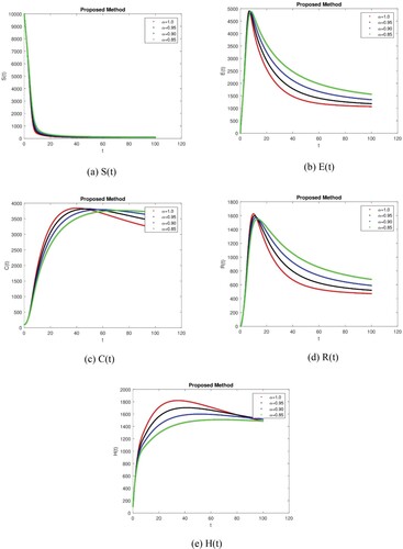
By using the Power-Law, Exponential Law, and Mittag-Leffler kernel techniques, we obtain the numerical simulation, and the graphs act for the numerical simulation results for the different values of $\alpha$ =  0.95, 0.90, 0.85, and 1.0. The numerical simulations in this section are used to study the temporal dynamical behaviour associated with the corruption using fractional-order parameters. It is critical to demonstrate the feasibility of the stated work and to test the validity of the analytical work using large-scale numerical simulation. The numerical results of the model for different fractional values are determined according to the steady-state point using different kernels. The model’s dynamics are affected by a change in value, according to these simulations. We can also see that compared to the traditional derivative, the fractional value results are more efficient in all three cases. We obtain the results as shown in Figure 1(a–e) by executing the Mittag-Lefler Kernel with the specified parameter values. Figure 1(a) shows that the susceptible individual decreases as fractional values decrease due to an increase in exposed and corrupt individuals. Figure 1(b,d) shows that the exposed and recovered individual increases and then decreases after a certain time and approaches its stable position as fractional values decrease but this stable position does not show its control position. Figure 1(c) shows that corrupt individuals increase and after a certain time it comes to a stable position due to campaigning shows that we may first stop to increase the corrupt people. Recovered individuals increase due to an increase in honest individuals and come to a stable position after a certain time, as shown in Figure 1(d,e). We obtain the results shown in Figure 2(a–e) by executing the Power-Law kernel with the specified parameter values. Similarly, we get the results shown in Figure 3(a–e) by executing the Exponential Law kernel with the specified parameter values. Similar behaviour can be seen in Figure 2(a–e) and in Figure 3(a–e) as can be seen in Figure 1(a–e) with minor effects. This shows that it requires more social media campaigns and punishment of corrupt individuals to stop corruption in society in all three cases. The graphical representation shows that over time, susceptible individual decreases due to an increase in corrupt people in all cases with minor effects. It indicates that we need to control corrupt individuals differently and need a strong punishment system to control it.

Figure 1. Simulation of all Compartments of the Corruption Model with the Mittag-Lefler Kernel using different fractional values.

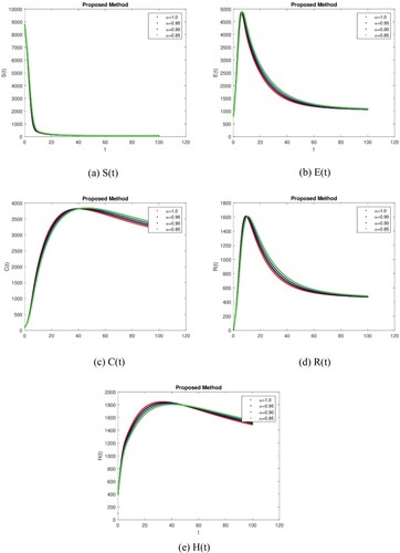
Figure 2. Simulation of all Compartments of the Corruption Model with the Power-Law kernel using different fractional values.

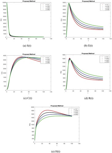
Figure 3. Simulation of all Compartments of the Corruption Model with the Exponential Law kernel using different fractional values.

5. Conclusion

We proposed a corruption model in this study to analyse corruption in society to check the dynamical behaviour of the system for constant controls with fractional operators. Positive and bounded solutions for corruption effects are verified. This research shows that the fractional operator approach provides more useful outputs on compartmental population dynamics than the classical model using different kernels. As a result, the Power-Law Kernel, Mittag-Leffler Kernel, and Exponential Decay Kernel can be concluded to be especially helpful for modelling real-world problems to analyse for efficient results. A numerical simulation is used to show the influence of fractional order to analyse its effects on the community using MATLAB. It is clear from the simulation that it affects the individual and corrupts group rises over time and we need a strong punishment process to overcome the effect of corruption. So, in order to overcome this habitual-minded and poverty factor-minded individual, it required anti-corruption campaigning through media and advertisements and putting corrupt people in jails and punishing them to make your society corruption free. To examine the actual action of corruption in the community, we execute the process of hanging.

Disclosure statement

No potential conflict of interest was reported by the author(s).

References

- Bahoo S, Alon I, Paltrinieri A. Corruption in international business: a review and research agenda. Int Bus Rev. 2020;29(4):101660.
- Cuervo-Cazurra A. Corruption in international business. J World Bus. 2016;51(1):35–49.
- Pontell HN, Geis G. International handbook of white-collar and corporate crime. Irvine, CA: Springer; 2007.
- Eguda F, Oguntolu F, Ashezua T. Understanding the dynamics of corruption using mathematical modeling approach. Int J Innov Sci Eng Technol. 2017;4(8):190–197.
- Heimann F, Boswell NZ. The OECD convention: milestone on the road to reform. New perspectives on combating corruption. p. 65–74. Washington: Transparency International; 1998.
- Alemneh HT. Mathematical modeling, analysis, and optimal control of corruption dynamics. J Appl Math. 2020;2020:Article ID 5109841, 1–13.
- Abdulrahman S. Stability analysis of the transmission dynamics and control of corruption. Pac J Sci Technol. 2014;15(1):99–113.
- Lemecha L. Modelling corruption dynamics and its analysis. Ethiop J Sci Sustain Dev. 2018;5(2):13–27.
- Waykar SR. Mathematical modelling: a comparatively mathematical Study model base between corruption and development. IOSR J Math. 2013;6(2):54–62.
- Nikolaev P. Corruption suppression models: the role of inspectors’ moral level. Comput Math Model. 2014;25(1):87–102.
- Khan MAU. The corruption prevention model. J Discrete Math Sci Cryptogr. 2000;3(1-3):173–178.
- Athithan S, Ghosh M, Li X-Z. Mathematical modeling and optimal control of corruption dynamics. Asian-Eur J Math. 2018;11(06):1850090.
- Nathan O, Jackob K. Stability analysis in a mathematical model of corruption in Kenya. Asian Res J Math. 2019;15(4):1–15.
- Caputo M. Linear models of dissipation whose Q is almost frequency independent—II. Geophys J Int. 1967;13(5):529–539.
- Atangana A, Baleanu D. New fractional derivatives with nonlocal and non-singular kernel: theory and application to heat transfer model. arXiv preprint arXiv:1602.03408, 2016.
- Mathale D, Goufo EFD, Khumalo M. Coexistence of multi-scroll chaotic attractors for a three-dimensional quadratic autonomous fractional system with non-local and non-singular kernel. Alexandria Eng J. 2021;60(4):3521–3538.
- Xu C, Farman M, Hasan A, et al. Lyapunov stability and wave analysis of Covid-19 omicron variant of real data with fractional operator. Alexandria Eng J. 2022;61(12):11787–11802.
- Ahmad S, Ullah A, Abdeljawad T, Akgül A, Mlaiki N, Analysis of fractal-fractional model of tumor-immune interaction, Results Phys, 2021;25:104178.
- Yu Y, Lihong H, Mouneer S, Ali H, Munir A. Foreign assistance, sustainable development and commercial law: a comparative analysis of the impact of corruption on developing economies. Front Environ Sci. 2022;10:959563. doi:10.3389/fenvs.2022.959563
- Abu-Gdairi R. Analytical solution of nonlinear fractional gradient-based system using fractional power series method. Int J Anal Appl. 2022;20:51.
- Al-Smadi, M., Arqub, O.A. and Gaith, M., Numerical simulation of telegraph and Cattaneo fractional-type models using adaptive reproducing kernel framework. Math Methods Appl Sci, 10(4), 2020, doi:10.1002/mma.6998
- Umar M, Sabir Z, Raja MAZ, et al. Neuro-swarm intelligent computing paradigm for nonlinear HIV infection model with CD4+ T-cells. Math Comput Simul. 2021;188:241–253.
- Abro KA, Atangana A, Francisco J, et al. An analytic study of bioheat transfer Pennes model via modern non-integers differential techniques. Eur Phys J Plus. 2021;136(11):1–11.
- Abro KA, Atangana A, Gómez Aguilar JF. A comparative analysis of plasma dilution based on fractional integro-differential equation: an application to biological science. Int J Model Simul. 2023;43(1):1–10.
- Li X, Agarwal RP, Gómez Aguilar JF, et al. Threshold dynamics: formulation, stability & sensitivity analysis of co-abuse model of heroin and smoking. Chaos, Solitons Fractals. 2022;161:112373.
- Takasar H, Ullah AA, Abro KA, et al. A passive verses active exposure of mathematical smoking model: a role for optimal and dynamical control. Nonlinear Eng. 2022;11(1):507–521.
- Jajarmi A, Baleanu D, Sajjadi SS, et al. Analysis and some applications of a regularized Hilfer fractional derivative. J Comput Appl Math. 2022;415:114476.
- Baleanu D, Ghassabzade FA, Nieto JJ, et al. On a new and generalized fractional model for a real cholera outbreak. Alexandria Eng J. 2022;61(11):9175–9186.
- Baleanu D, Abadi MH, Jajarmi A, et al. A new comparative study on the general fractional model of COVID-19 with isolation and quarantine effects. Alexandria Eng J. 2022;61(6):4779–4791.
- Jajarmi A, Baleanu D, Vahid KA, et al. A new and general fractional Lagrangian approach: a capacitor microphone case study. Results Phys. 2021;31:104950.
- Erturk VS, Godwe E, Baleanu D, et al. Novel fractional-order Lagrangian to describe motion of beam on nanowire. Acta Phys Pol A. 2021;140(3):265–272.
- Tajadodi H, Khan A, Francisco Gómez-Aguilar J, et al. Optimal control problems with Atangana-Baleanu fractional derivative. Optim Control Appl Methods. 2021;42(1):96–109.
- Khan H, Alam K, Gulzar H, et al. A case study of fractal-fractional tuberculosis model in China: existence and stability theories along with numerical simulations. Math Comput Simul. 2022;198:455–473.
- Begum R, Tunç O, Khan H, et al. A fractional order Zika virus model with Mittag–Leffler kernel. Chaos, Solitons Fractals. 2021;146:110898.
- Khan H, Begum R, Abdeljawad T, et al. A numerical and analytical study of SE (Is)(Ih) AR epidemic fractional order COVID-19 model. Adv Differ Equ. 2021;2021(1):1–31.
- Ahmad H, Khan MN, Ahmad I, et al. A meshless method for numerical solutions of linear and nonlinear time-fractional Black-Scholes models. AIMS Math. 2023;8(8):19677–19698.
- Ahmad H, Ozsahin DU, Farooq U, et al. 2023.
- Khaliq S, Ahmad S, Ullah A, et al. New waves solutions of the (2+1)-dimensional generalized Hirota–Satsuma–Ito equation using a novel expansion method. Results Phys. 2023;50:106450.
- Qayyum M, Ahmad E, Tauseef Saeed S, et al. Homotopy perturbation method-based soliton solutions of the time-fractional (2 + 1)-dimensional Wu–Zhang system describing long dispersive gravity water waves in the ocean. Front Phys. 2023;11:1178154.
- Adel M, Khader MM, Ahmad H, et al. Approximate analytical solutions for the blood ethanol concentration system and predator-prey equations by using variational iteration method. AIMS Math. 2023;8(8):19083–19096.
- Ullah I, Ullah A, Ahmad S, et al. A survey of KdV-CDG equations via nonsingular fractional operators. AIMS Math. 2023;8(8):18964–18981.