Predicting COVID-19 outbreak in India using modified SIRD model

Abstract

In this paper, the existing Susceptible-Infected-Recovered-Deceased (SIRD) compartmental epidemiologic process model is modified for forecasting the coronavirus effect in India. The data from India was studied for weekly fatalities, weekly infected, weekly recovered, new cases, infected and recovered individuals, Reproductive Number $R_0$, recovery rate, death rate, and coefficient of transmission from 30 January 2020 to 31 July 2021. SARS Coronavirus 2 (SARS-CoV-2) is the Covid strain that causes Covid sickness (COVID-19), a respiratory ailment that triggered the outbreak of COVID-19 at the beginning of December 2019. We aim to provide a hybrid SIRD model for predicting the COVID-19 outbreak. In the proposed method, to improve the exploration ability of the Grey Wolf Optimizer (GWO) or to avoid stagnation in the swarm, a modified Grey Wolf Optimization Algorithm is used to optimize the initial value of Infected individuals. The modified SIRD model is further applied to get the predicted values. The data is examined on weekly basis to prevent noise. Depending on the fact, that the precise mode of transmission is highly dependent on how and when different precautions such as isolation, confinement, and other preventative measures were implemented, we put together our projections concerning satisfactory speculations based on genuine realities. The experimental results show the various trends observed in the pandemic in terms of number of peaks, increasing trend, decreasing trend, and continuous trend for infected individuals, weekly change in number of cases, weekly deaths, weekly infected, and weekly recoeverd cases of Covid-19. The proposed modified SIRD model could be a valuable tool for assessing the impact of government measures on COVID-19 outbreak.

KEYWORDS:

• COVID-19
• epidemiology
• grey wolf optimizer
• reproductive number

MATHEMATICS SUBJECT CLASSIFICATIONS:

• 92-10
• 65K10
• 90C31
• 92D30

1. Introduction

An infectious disease caused by the virus SARS-CoV-2 is known as COVID-19 or Coronavirus disease. Depending upon the symptoms, a person infected with this virus may experience benign or severe respiratory ailment. COVID-19 is likely to cause extreme conditions in older people with previous medical history such as diabetes, cancer, or cardiovascular disease [1]. The COVID-19 virus can be best envisioned with the help of the SIRD compartmental model [2].

The Susceptible-Infected-Recovered-Deceased (SIRD) is a compartmental epidemiological procedure model [3] used to study epidemics. This model has been incorporated to analyse the data in this paper. One of the most general mathematical modelling techniques for infectious diseases is the Compartmental model. The compartments have the labels such as $\mathrm{Susceptible}(S)$, $\mathrm{Infectious}(I)$, or $\mathrm{Recovered}(R)$, which are assigned the population. There may be chances of progress amidst compartments. The flow patterns among the different compartments can be visualized with the help of the order of the labels given [4]. For example, susceptible, exposed, infectious, then susceptible again, follow the pattern SEIS [5].

Many researchers have used the SIRD model for analysing the situation of COVID-19 worldwide. Coccavo [6] used the SIRD model to predict the impact of COVID-19 in China and Italy. Calafiore et al. [7] used a time-varying SIRD model for predicting the COVID-19 contagion in Italy by using the official data to identify the model parameters. Sen and Sen [8] used the modified SIRD model to analyse the time-series data of COVID-19 for China, Italy, France, the United States, and India. Khajanchi et al. [9] performed a sensitivity analysis using partial rank correlation coefficients approaches to determine the most effective parameters. By using the least squares method, the value of those sensitive parameters was calculated from the observed data. To find out how important the system parameters are in relation to one another, they conducted sensitivity analysis. To assess how resistant the model predictions are to parameter values, they also computed the sensitivity indices.

To evaluate the effectiveness of social media advertising in containing the coronavirus pandemic in India, Rai et al. [10] provided a mathematical model. They calibrated the suggested model using India's total number of confirmed COVID-19 cases. Eight epidemiologically significant factors were estimated, along with the size of India's basic reproduction number, in their study. Samui et al. [11] proposed a SAIU compartmental mathematical model to account for the COVID-19 transmission dynamics. They analysed local and global stability for the endemic and infection-free equilibrium point. Also, to determine the factors that are most useful in relation to the fundamental reproduction number R0, a sensitivity analysis is carried out. Khajanchi and Sarkar [12] created a brand-new compartmental model that clarifies the COVID-19 transmission kinetics. With daily COVID-19 data for four Indian states–Jharkhand, Gujarat, Andhra Pradesh, and Chandigarh–they calibrated their model. They examined the model's qualitative characteristics, including the model's possible equilibria and their stability with regard to the fundamental reproduction number R0.

Sarkar et al. [13] proposed a SARIIqSq compartmental mathematical model to account for the COVID-19 transmission dynamics. They determined the most sensitive parameters by doing a PRCC analysis, based on actual data up to 30 April 2020. To determine the most efficient parameters in relation to the fundamental reproduction number R0, a sensitivity analysis was carried out in their work. Khajanchi et al. [14] used the susceptible-exposed-infectious-recovered model, which was improved using contact tracing and hospitalisation data from the Indian provinces of Kerala, Delhi, Maharashtra, and West Bengal, as well as from India as a whole. They determined The most important input parameters through sensitivity analysis, and the model has been calibrated to provide the most accurate description of the data. Long-term projections also indicate the probability of oscillatory dynamics, while short-term predictions indicate an increasing and concerning trend in COVID-19 instances for all four provinces and India as a whole.

Ghosh et al. [15] applied the regression methods for capturing the competing risks to COVID-19. The cause-specific and sub-distribution risks regression techniques, which are applied to the COVID-19 incidence data from the USA, are the methods that are most frequently utilized in their work. Ghosh et al. [16], in order to demonstrate relative risks and cumulative mortality rates using COVID-19 data from Spain, they first devised a non-parametric technique for odds ratios with appropriate confidence intervals (CIs). Using the Italian COVID-19 data, they have shown how the modified non-parametric approach based on the Kaplan-Meier (KM) algorithm works. Additionally, they looked at the importance of patient characteristics in relation to outcome by age for both genders. Saha et al. [17] employed control measures to lessen the illness burden, for which, an optimal control problem is taken into account. Numbers demonstrate that the behavioural response control first operates with greater intensity after deployment before gradually waning over time.

Susceptible (S), asymptomatic infected (A), clinically ill or symptomatic infected (I), quarantine (Q), isolation (J), and recovered (R) are the six stages of infection that were taken into consideration by Mondal and Khajanchi [18]. These six stages are generally referred to as SAIQJR. In terms of the fundamental reproduction number, the qualitative behaviour of the model and the stability of biologically plausible equilibrium points are examined. With regard to the fundamental reproduction number, they conducted sensitivity analysis and discovered that the illness transmission rate has an effect on preventing the spread of diseases. Tiwari et al. [19] derived the expression for fundamental reproduction number. They established the necessary criteria for endemic equilibrium to be stable globally. To determine the essential model parameters that have a significant impact on the prevalence and management of COVID-19, sensitivity analysis was performed. They modified the suggested model to meet the COVID-19 case data set for India. They provided the simulation results which demonstrate that spreading awareness among vulnerable people at the community and individual levels is essential for preventing the COVID-19 disease.

In the scenario of COVID-19, once infected, a person either heals or dies. Our approach, unlike the traditional version, is based on the following presumptions:

1. Every individual transition between the compartments is dynamic and therefore dependent on time.

2. Time-dependency is directly impacted by the frequency of non-pharmaceutical inferences. As a result, estimating a comparable reduction in the disease's transmission rate may be useful in assessing how well these conclusions performed.

This work is an extension of our previous work on Covid-19 [20], where we intend to analyse the weekly data as our future scope. The proposed model is used to examine the evolution of COVID-19 [21]. This methodology has been adopted by 35 Indian States and Union-Territories (UTs). Susceptible (S), Infected (I), Recovered (R), and Dead (D) are the four stages of infection that the model goes through.

To identify the initial value of Infected individuals, we have used Grey Wolf Optimization (GWO) algorithm. GWO [22] is a recent nature-inspired algorithm that imitates the behaviour of grey wolves. It consists of the alpha (α), beta (β), omega (ω), and delta (δ), forming the four main classes of the GWO. GWO works on four phases: encircling the prey, hunting the prey, attacking the prey (exploitation), and searching for prey (exploration).

The paper is structured as follows: Model structure and method are described in Section 2. Results analysis is covered in Section 3. The conclusion is presented in Section 4.

2. Model structure and method

The total population P [23] at time t comprises of the total number of $\mathrm{Susceptible}(S_t)$, $\mathrm{Infected}(I_t)$, $\mathrm{Recovered}(R_t)$, and $\mathrm{Dead}(D_t)$ individuals.

2.1. The SIRD model

Equation (1(1) $P_t=S_t+I_t+R_t+D_t$(1) ) computes the value of total population $P_t$: (1) $P_t=S_t+I_t+R_t+D_t$(1) Equation (2(2) $C_t=I_t+R_t+D_t$(2) ) computes the change in the cases reported: (2) $C_t=I_t+R_t+D_t$(2) An approximately constant value is estimated by Equation (1(1) $P_t=S_t+I_t+R_t+D_t$(1) ). The value of $S_t$, $I_t$, $R_t$, and $D_t$ is computed using the following equations: (3) $\begin{array}{rl}{S}_{t+1}& =S_t-\left(\frac{{\beta }_t{S}_t{I}_t}{P_t}\right)\end{array}$(3) (4) $\begin{array}{rl}{I}_{t+1}& =I_t+\left(\frac{{\beta }_t{S}_t{I}_t}{P_t}\right)-\gamma I_t-\delta I_t\end{array}$(4) (5) $\begin{array}{rl}{R}_{t+1}& =R_t+{\gamma }_t{I}_t\end{array}$(5) (6) $\begin{array}{rl}{D}_{t+1}& =D_t+{\delta }_t{I}_t\end{array}$(6) At the beginning, the total susceptibles $(S_t)$ individuals were approximately equivalent to the total polulation $(P_t)$. Equations (7(7) $\begin{array}{rl}{r}_0& ={\beta }_t-({\gamma }_t+{\delta }_t)\end{array}$(7) ) and (8(8) $\begin{array}{rl}{R}_0& =\frac{{\beta }_t}{{\gamma }_t+{\delta }_t}\end{array}$(8) ) computes the per week exponential growth rate $(r_0)$ and the underlying dimensionless Reproductive Number $(R_0)$ [24]: (7) $\begin{array}{rl}{r}_0& ={\beta }_t-({\gamma }_t+{\delta }_t)\end{array}$(7) (8) $\begin{array}{rl}{R}_0& =\frac{{\beta }_t}{{\gamma }_t+{\delta }_t}\end{array}$(8) If the value of $R_0>1(r_0>0)$, the COVID-19 pandemic progresses, or else crumbles.

2.2. Effects of government interventions 25–32 on COVID-19 outbreak

Suppose that the weekly change in susceptible individuals is computed as $\mathrm{\Delta }S=S_{t+1}-S_t$. where,

$S_t$ stands for average number of susceptible at $t^{\mathrm{th}}$ week (average of 7 days data ending at the end of week t (included))

$S_{t+1}$ stands for average number of susceptible at $(t+1{)}^{\mathrm{th}}$ week (average of 7 days data, counting from next day from the end of week t), $t=0,1,2,\dots$ Here $S_0$ = 0

Equations (9(9) $\begin{array}{rl}\mathrm{\Delta }S& =\frac{-{\beta }_t{S}_t{I}_t}{P_t}\end{array}$(9) )–(12(12) $\begin{array}{rl}\mathrm{\Delta }D& ={\delta }_t{I}_t\end{array}$(12) ) computes the weekly change of Infected, Recovered, and Deceased individuals: (9) $\begin{array}{rl}\mathrm{\Delta }S& =\frac{-{\beta }_t{S}_t{I}_t}{P_t}\end{array}$(9) (10) $\begin{array}{rl}\mathrm{\Delta }I& =\left(\frac{{\beta }_t{S}_t{I}_t}{P_t}\right)-{\gamma }_{t}I-{\delta }_{t}I\end{array}$(10) (11) $\begin{array}{rl}\mathrm{\Delta }R& ={\gamma }_t{I}_t\end{array}$(11) (12) $\begin{array}{rl}\mathrm{\Delta }D& ={\delta }_t{I}_t\end{array}$(12) The above equations are used to determine the transmission coefficient, recovery rate, and death rate.

The change in the number of total cases (2(2) $C_t=I_t+R_t+D_t$(2) ) was very less in comparison to the total population $P_t$. This leads to making the total population nearly equal to susceptible individuals and hence ${\beta }_t=\mathrm{\Delta }C/I_t$. In the case of large data, such as used in our work from 30 January 2020 to 31 July 2021, a modified SIRD model is requisite, to calculate the near accurate values as $C_t$ is large. In the modified SIRD model the equation of transmission coefficient is modified and computed as: From Equation (9(9) $\begin{array}{rl}\mathrm{\Delta }S& =\frac{-{\beta }_t{S}_t{I}_t}{P_t}\end{array}$(9) ), (13) $\mathrm{\Delta }{I}_t+\gamma t{I}_t+{\delta }_t{I}_t=\frac{{\beta }_t{S}_t{I}_t}{P_t}$(13) From Equations (2(2) $C_t=I_t+R_t+D_t$(2) ), (11(11) $\begin{array}{rl}\mathrm{\Delta }R& ={\gamma }_t{I}_t\end{array}$(11) ) and (12(12) $\begin{array}{rl}\mathrm{\Delta }D& ={\delta }_t{I}_t\end{array}$(12) ), (14) $\mathrm{\Delta }{C}_t=\frac{{\beta }_t{S}_t{I}_t}{P_t}$(14) From Equation (1(1) $P_t=S_t+I_t+R_t+D_t$(1) ), (15) $\begin{array}{rl}\mathrm{\Delta }{C}_t& =\frac{{\beta }_t(P_t-C_t)I_t}{P_t}\end{array}$(15) (16) $\begin{array}{rl}{\beta }_t& =\left(\frac{\mathrm{\Delta }{C}_t}{I_t}\right)\ast P_t/(P_t-C_t)\end{array}$(16) (17) $\begin{array}{rl}{\gamma }_t& =\frac{\mathrm{\Delta }{R}_t}{I_t}\end{array}$(17) (18) $\begin{array}{rl}{\delta }_t& =\frac{\mathrm{\Delta }{D}_t}{I_t}\end{array}$(18) The value of the transmission coefficient will be less when the total population is equal to susceptible individuals $(P_t=S_t)$, resulting in low $R_0$ values as compared to the beta values procured by taking $P_t=S_t+C_t$, which results in higher $R_0$ values. This concludes to imprecise predictions when $P_t=S_t$, exclusively when $R_0$ is relatively 1.

The values of $P_t$, $C_t$, $I_t$, $R_t$, and $D_t$ can be used to compute the SIRD parameters.

The COVID-19 pandemic can be analysed using the parameters specified in Table 1.

Table 1. The SIRD model parameters.

S. No.	Parameter	Definition
1.	$P_t$	India's Population
2.	$S_t$	Number of Susceptible Individuals
3.	$I_t$	Number of Infected Individuals
4.	$R_t$	Number of Recovered Individuals
5.	$D_t$	Total Deaths
6.	$C_t$	Change in cases reported
7.	${\beta }_t$	Transmission Coefficient
8.	${\gamma }_t$	Recovery Rate of Individuals
9.	${\delta }_t$	Death Rate of Individuals

The tremendous amount of noise, in terms of process and measurement, can be seen in the values of the parameters due to the following reasons: The infected individuals were relatively less at the beginning of the pandemic, resulting in high process noise. The disruption in reporting of daily cases and the misclassification and misunderstanding of COVID-19 cases by the government authorities may result in higher measurement noise. The process of data smoothing may help to reduce the process and measurement noise.

2.3. Model requirements

2.3.1. Description of dataset

The dataset from 30 January 2020 to 31 July 2021, is collected from COVID19 INDIA [33]. The data collected is unforeseen eminently, as a result of reliance on physical variables for increase or decrease in total cases. The dataset contains 35 absolute time-series data for the number of confirmed, recovered, and deceased cases recorded in each of India's states and union territories. Table 2 consists of the dataset values, where 1L = ${10}^5$ and, 1Cr = ${10}^7$.

Table 2. Dataset (30 January 2020 to 31 July 2021).

S. No.	State/UT Name	Confirmed(C)	Recovered(R)	Deceased(D)	Tested	Population (P)
1.	Andaman and Nicobar Islands	7537	7400	129	440,870	4L
2.	Andhra Pradesh	1,966,175	1,931,618	13,377	24,563,043	5.2Cr
3.	Arunachal Pradesh	48,122	43,939	299	938,932	15.33L
4.	Assam	566,198	547,616	5260	18,631,110	3.50Cr
5.	Bihar	724,835	714,735	9643	37,351,795	12.30Cr
6.	Chandigarh	61,953	61,111	811	613,891	12L
7.	Chhattisgarh	1,002,008	986,621	13,524	11,394,233	2.95Cr
8.	Delhi	1,436,265	1,410,631	25,053	23,666,237	2Cr
9.	Dadra and Nagar Haveli & Daman and Diu	10,653	10,586	4	72,410	10.77L
10.	Goa	171,146	166,941	3147	1,056,184	16L
11.	Gujarat	824,877	814,549	10,076	25,554,891	7Cr
12.	Himachal Pradesh	206,027	201,270	3505	2,834,431	74L
13.	Haryana	769,913	759,566	9635	10,874,081	2.95Cr
14.	Jharkhand	347,173	341,793	5128	11,661,115	3.85Cr
15.	Jammu and Kashmir	321,462	315,908	4378	11,718,976	1.34Cr
16.	Karnataka	2,905,124	2,844,742	36,562	38,649,498	6.70Cr
17.	Kerala	3,390,761	3,208,969	16,781	27,217,010	3.55Cr
18.	Ladakh	20,338	20,075	207	435,897	2.97L
19.	Maharashtra	6,303,715	6,090,786	132,791	47,967,609	12.44Cr
20.	Meghalaya	65,000	57,949	1085	844,473	33L
21.	Manipur	98,499	86,403	1556	1,086,940	31.65L
22.	Madhya Pradesh	791,828	781,193	10,513	14,427,356	8.45Cr
23.	Mizoram	38,064	26,387	148	616,223	12.16L
24.	Nagaland	27,872	25,193	566	263,703	22L
25.	Odisha	977,268	956,828	5955	16,022,677	4.55Cr
26.	Punjab	599,104	582,277	16,293	12,129,632	3Cr
27.	Puducherry	120,915	118,158	1795	1,504,306	15.71L
28.	Rajasthan	953,667	944,465	8954	12,935,008	7.92Cr
29.	Sikkim	26,548	22,535	344	200,688	6.77L
30.	Tamil Nadu	2,559,597	2,504,805	34,076	37,446,148	7.65Cr
31.	Telangana	644,951	632,080	3802	22,006,215	3.52Cr
32.	Tripura	78,358	74,059	752	1,559,001	41L
33.	Uttar Pradesh	1,708,441	1,684,973	22,756	65,502,631	23Cr
34.	Uttarakhand	342,139	328,108	7362	6,298,254	1.14Cr
35.	West Bengal	1,528,019	1,498,770	18,136	15,730,474	9.8Cr

Source: covid19india.org.

2.3.2. Methodology

The computed time-series of weekly data can be used to further evaluate the time-series data of the following:

1. The number of New Cases (19) $\mathrm{\Delta }C=C_{t+1}-C_t$(19)

2. The number of Infecetd/Active Cases (20) $\mathrm{\Delta }I=C_t-(R_t+D_t)$(20)

3. The number of Weekly Deaths (21) $\mathrm{\Delta }D=D_{t+1}-D_t$(21)

SIRD parameters weekly estimates can be computed by using the above equations.

In our approach, we have used Locally Weighted Scatterplot Smoothing (LOWESS) [34], for smoothing of data. LOWESS is a famous tool that draws a smooth line over a timeplot/scatterplot witnessing the relationship among the variables and predictive trends. It is used in Regression Analysis. In order to move closer to the straight line rather than curves, a fraction of 0.1 is estimated for ${\beta }_i$ and δ and a fraction of 0.2 is estimated for γ.

Since for small values, the data is excessively noisy, the smoothing of parameters is only applied as soon as $C_t$ surpasses 100 cases. A constant value is assigned to $C_t$ until it attains 100 cases and is assigned a value equivalent to the first value smoothed.

The modified SIRD model is calculated ahead of time for time period of the pandemic, by smoothing the model parameters. Suppose the initial values of the SIRD model as S(0)= N, R(0)=D(0)=0, and the optimal value of I(0) is obtained using the Modified Grey Wolf Optimizer (GWO) Algorithm.

3. Formulation of optimization problem for initial value of infected individuals ($I_0$)

The initial value of Infected individuals $I_0$ can be obtained in different ways with the help of the data. Finding the most suitable value of $I_0$ is very challenging. We have used the optimization method to obtain the initial I. The Modified GWO is used to identify the optimal initial value of the infected individuals ($I_0$), so that the mathematically generated data is near the real reported data.

3.1. Grey wolf optimizer (GWO)

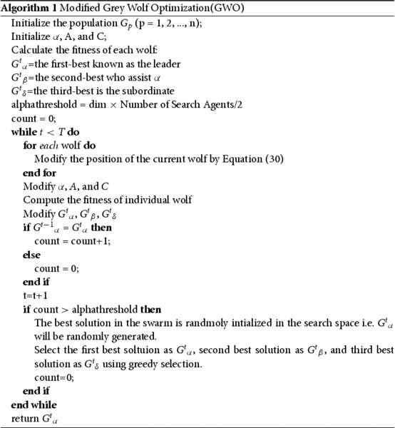
The GWO algorithm developed by Mirjalili [22] is a population-based metaheuristic algorithm, designed to explore and construct a heuristic (partial search algorithm), to find an optimal solution for any optimization problem. All the algorithms with randomization and local search capacity are known as metaheuristic algorithm [35]. Metaheuristic algorithms can relatively handle problems with a huge population [36]. Unlike other optimization algorithms, metaheuristic algorithms do not assure to obtain the optimal solution, but they are capable of computing sub-optimal, good-quality solutions and take feasible execution time [37]. GWO is one such type of metaheuristic algorithm that mimes the attacking behaviour and management hierarchy of grey wolves. In GWO, to fabricate the management hierarchy, the colony of wolves is divided into primarily four main classes, alpha (α), beta (β), omega (ω) and delta (δ). The alpha wolf is the leader and considered the best ones. They are responsible for making decisions for hunting, time to sleep, waking up time and so on. Beta is the second-level wolves. They are the auxiliary wolves that help alpha wolves in decision-making and other activities. Delta is the third-best, and it is responsible for sacrifice. These wolves are responsible for dominating other wolves. Omega is the lowest-ranked grey wolves. They are considered as the weaklings and are ready to sacrifice. All other wolves are delta wolves.

The working of GWO can be described in the following four steps:

1. Encircling prey

2. Hunting

3. Attacking prey (Exploitation)

4. Search prey (Exploration)

The mathematical model for hunting the prey, attacking on the prey, and to search the prey is described in this section.

3.1.1. Encircling prey

The encircling of prey by the grey wolves is given mathematically by the following equations: (22) $\begin{array}{rl}D& =\mid C.{G^t}_{\mathrm{prey}}-G^t\mid \end{array}$(22) (23) $\begin{array}{rl}{G}^{t+1}& ={G^t}_{\mathrm{prey}}-A\ast D\end{array}$(23) (24) $\begin{array}{rl}A& =2\ast a\ast r_1-a\end{array}$(24) (25) $\begin{array}{rl}a& =2-2\left(\frac{t}{T}\right)\end{array}$(25) (26) $\begin{array}{rl}C& =2\ast r_2\end{array}$(26) where t denotes the current iteration, vector A and C indicates coefficient vectors. $G_{\mathrm{prey}}$ and G indicates the position of prey and grey wolf respectively. a is a vector which linearly decreases from 2 to 0 over the course of iterations. $r_1$ and $r_2$ are random vectors in the range [0,1]. Initially, vector A has a maximum value, which decreases gradually as the iterations increase which can be calculated by Equation (6(6) $\begin{array}{rl}{D}_{t+1}& =D_t+{\delta }_t{I}_t\end{array}$(6) ). I indicates the maximum number of iterations.

3.1.2. Hunting

To mathematically simulate the hunting behaviour of grey wolves, the α, β, and δ are considered as the best solution which possesses better information about the location of prey (optimal). Based on this information, other grey wolves update their positions using the following equations [22] : (27) $\begin{array}{rl}{G}_1& ={G^t}_{\alpha }-A_1\ast D_{\alpha }\end{array}$(27) (28) $\begin{array}{rl}{G}_2& ={G^t}_{\beta }-A_2\ast D_{\beta }\end{array}$(28) (29) $\begin{array}{rl}{G}_3& ={G^t}_{\delta }-A_3\ast D_{\delta }\end{array}$(29) where, (30) $\begin{array}{rl}{D}_{\alpha }& =\mid C_1.{G^t}_{\alpha }-G\mid D_{\beta }=\mid C_2.{G^t}_{\beta }-G\mid D_{\delta }=\mid C_3.{G^t}_{\delta }-G\mid \\ G^{t+1}& =\frac{G_1+G_2+G_3}{3}\end{array}$(30)

3.1.3. Attack on prey (Exploitation) and search prey (Exploration)

The exploitation and exploration behaviour in the GWO algorithm, depends upon the A and C parameters. A is a random value in the range [-a,a]. The wolf shows exploration behaviour when $\mid A\mid$ >1 and C >1, whereas exploitation occurs when $\mid A\mid$ <1 and C <1.

To improve the exploration ability of the GWO or to avoid stagnation in the swarm, a modified solution search strategy is proposed in this section. As the whole swarm is attracted towards the best prey ${G^t}_{\alpha }$, so on the basis of ${G^t}_{\alpha }$ location, there may be a situation that the swarm may converge to local optima or may stuck at some other location in the search space. To avoid this situation, a fluctuation is introduced in the swarm i.e. the ${G^t}_{\alpha }$ solution is randomly generated in the swarm, if it is not updating itself up to a predefined number of iterations named as ‘alphathreshold’ and in next-generation, the first, second, and third best solutions are selected as ${G^t}_{\alpha }$, ${G^t}_{\beta }$, and ${G^t}_{\delta }$ respectively. Hence, it is expected that the exploration ability of the GWO will be improved, and the same is proved through experiments.

The following values of Modified GWO are taken into consideration for calculations:

–	Objective Function: $\mathrm{pred}{R}^2$
–	Lower and Upper Bound: 0 and 200,000 respectively
–	Dimensions: One-Dimensional
–	Number of Search Agents: 16
–	Maximum Iterations (T): 100

Algorithm 1 describes the pseudo-code of the Modified GWO algorithm:

The steps of the algorithm are illustrated below:

To measure how fit is our model, we have estimated the coefficient of prediction $\mathrm{pred}{R}^2$ by Equation (31(31) $\mathrm{pred}{R}^2=1-\frac{\sum (Y-X{)}^2}{\sum [X-\mathrm{mean}(X){]}^2}$(31) ) (31) $\mathrm{pred}{R}^2=1-\frac{\sum (Y-X{)}^2}{\sum [X-\mathrm{mean}(X){]}^2}$(31) where:

The data is given by X and the number of confirmed and recovered cases for model prediction is given by Y.

If the model predictions are worst in comparison to the data mean, the value of $\mathrm{pred}{R}^2$ may be negative. The prediction is near to accurate if $\mathrm{pred}{R}^2$ reaches 1.

The value of $\mathrm{pred}{R}^2$, before and after smoothing of model parameters is given in Table 3. On the basis of obtained values after smoothing of model parameters, we can observe that the proposed model fits best on the given data. The model does not fit on Ladakh due to the inconsistency in data.

Table 3. Comaprative analysis of $\mathrm{pred}{R}^2$ for all States/UT of India.

		SIRD Model		Modified SIRD Model
		$\mathrm{pred}{R}^2$	$\mathrm{pred}{R}^2$	$\mathrm{pred}{R}^2$	$\mathrm{pred}{R}^2$
S. No.	Name of States/UT	(Without Smoothing)	(With Smoothing)	(Without Smoothing)	(With Smoothing)
1.	Andaman & Nicobar Islands	-2.2535	0.9911	-2.2536	0.9928
2.	Andhra Pradesh	-763.534	0.9307	-706.769	0.9838
3.	Arunachal Pradesh	-1.389	0.6703	-1.389	0.5642
4.	Assam	-1.6026	0.9407	-1.6026	0.9512
5.	Bihar	0.5249	-0.9823	0.5237	0.9823
6.	Chandigarh	-19.5078	0.9751	-9.9129	0.9274
7.	Chhattisgarh	-0.7894	0.9436	-0.7905	0.923
8.	Dadra and Nagar Haveli & Daman and Diu	-1.3166	0.9451	-1.3166	0.9324
9.	Delhi	0.3597	0.9548	-0.9777	0.8402
10.	Goa	-1.0153	0.8442	-1.0158	0.9896
11.	Gujarat	-0.3128	0.915	-0.2961	0.9306
12.	Haryana	-2.4522	0.9564	-2.4453	0.9786
13.	Himachal Pradesh	-504.687	0.956	-0.470.059	0.9724
14.	Jammu and Kashmir	-67.8436	0.9486	-63.0222	0.9714
15.	Jharkhand	-242.28	0.9813	-233.451	0.9798
16.	Karnataka	-3.0378	0.9786	-0.2.5741	0.9859
17.	Kerala	-280.866	0.8634	-275.396	0.953
18.	Ladakh	-286.159	-0.0889	-285.743	-0.0891
19.	Madhya Pradesh	-47.2363	0.9387	-0.48.0018	0.948
20.	Maharashtra	0.9676	0.9493	0.9904	0.986
21.	Manipur	-17.8159	-4849.89	-1.0679	0.916
22.	Meghalaya	-0.8079	0.9821	-0.808	0.9853
23.	Mizoram	-0.5213	0.9496	-0.5212	0.9428
24.	Nagaland	-1.4135	0.9897	-1.4136	0.9888
25.	Odisha	-12.6133	0.9764	-10.3565	0.9504
26.	Puducherry	-0.1407	0.8833	-0.0172	0.9848
27.	Punjab	-0.0304	0.9843	0.0354	0.9818
28.	Rajasthan	-0.6856	0.9763	-0.6819	0.9794
29.	Sikkim	-0.1812	0.991	-0.2027	0.9861
30.	Tamil Nadu	-4.3895	0.9882	-3.1724	0.9817
31.	Telangana	-6835.37	0.9816	-7408.93	0.991
32.	Tripura	-1.3802	0.9142	-1.3994	0.9337
33.	Uttar Pradesh	-0.4712	0.9883	-0.4713	0.9883
34.	Uttarakhand	-1347.91	0.989	-1338.79	0.9918
35.	West Bengal	0.5845	0.9944	0.607	0.9967

4. Experimental results

On 30 January 2020, the first case in India of Covid-19 was reported to WHO [38]. This section illustrates the detailed analysis of peaks and recent trends of Infected individuals, weekly change in number of cases, weekly deaths, weekly infected and weekly recoeverd cases of Covid-19, in tabular and graphical form.

4.1. Analysis of peaks and recent trends

The Table 4 below illustrates the Peaks and Recent Trends of Infected individuals, weekly change in number of cases, weekly deaths, weekly infected and weekly recoeverd cases of Covid-19 in India from the beginning to July 31, 2021. Here,

–	Numbers (1,2,3): Specifies the number of peaks
–	Upward Arrow (↑): Specifies increasing trend
–	Downward Arrow (↓): Specifies decreasing trend
–	Right Arrow ($\to$): Specifies a continuous trend
–	AD: Abruptly Down last value
–	NM: Not Matching; data and continuous curve

Table 4. Peaks and recent trends.

S. No.	State/UT	I	$\mathrm{\Delta }C$	$\mathrm{\Delta }D$	$\mathrm{\Delta }I$	$\mathrm{\Delta }R$
1.	Andaman & Nicobar Islands	2 ↓	3 ↓	3 ↓	2 $\to$	2 ↓
2.	Andhra Pradesh	2 ↓	2 ↓	2 ↓	2 ↑	2 ↓
3.	Arunachal Pradesh	2 ↑	3 ↓	2 ↑	3 ↓	3 ↓
4.	Assam	2 ↓	2 ↓	1 ↓	1 $\to$	2 ↓
5.	Bihar	2 ↓	2 ↓	2 ↓	2 ↑	2 ↓
6.	Chandigarh	3 ↓	3 ↓	3 ↓	3 ↑	3 ↓
7.	Chhattisgarh	2 ↓	2 ↓	2 ↓	3 ↑	2 ↓
8.	Dadra and Nagar Haveli & Daman and Diu	2 ↓	2 ↓	2 $\to$	2 ↑	2 ↓
9.	Delhi	4 ↓	4 ↓	3 ↓	4 $\to$	4 $\to$
10.	Goa	2 ↓	2 ↓	2 ↓	2 ↑	2 ↓
11.	Gujarat	2 ↓	3 ↓	4 ↓	1 ↑	2 ↓
12.	Haryana	3 ↓	3 ↓	4 ↓	3 ↑	3 ↓
13.	Himachal Pradesh	3 ↓	3 ↓	3 ↓	3 ↑	3 ↓
14.	Jammu and Kashmir	2 ↓	2 ↓	3 ↓	4 ↑	2 ↓
15.	Jharkhand	2 ↓	2 ↓	2 ↓	2 ↑	2 ↓
16.	Karnataka	2 ↓	2 ↓	2 ↓	1 ↑	2 ↓
17.	Kerala	3 ↑	3 ↓	2 ↓	3 ↑	3 ↓
18.	Ladakh	3 ↓	2 ↓	No Pattern ↓	No Pattern ↑	3 ↓
19.	Madhya Pradesh	3 ↓	3 ↓	3 ↓	3 ↑	3 ↓
20.	Maharashtra	2 ↓	2 ↓	3 ↓	3 ↑	2 ↓
21.	Manipur	2 ↑	3 ↓ AD	3 ↓ AD	No pattern ↑	No Pattern AD ↓
22.	Meghalaya	3 ↓	2 ↓	2 ↓	2 ↓	2 ↓
23.	Mizoram	3 ↑	2 ↓ AD	No Pattern ↓	No Pattern ↓	3 ↓ AD
24.	Nagaland	3 ↑	4 ↓	3 ↓	No Pattern ↓	3 ↓
25.	Odisha	2 ↓	2 ↓	2 ↓ AD	2 ↑	2 ↓
26.	Puducherry	2 ↓	2 ↓	2 ↓	2 ↑	2 ↓
27.	Punjab	3 ↓	3 ↓	3 ↓	3 ↑	3 ↓
28.	Rajasthan	2 ↓	2 ↓	2 ↓	1 ↑	2 ↓
29.	Sikkim	3 ↑	3 ↓ AD	No Pattern ↓	No Pattern ↑	3 ↓ AD
30.	Tamil Nadu	2 ↓	2 ↓	2 ↓	2 ↑	2 ↓
31.	Tripura	3 ↓	3 ↓	2 ↓	No Pattern ↓	3 ↓ AD
32.	Telangana	2 ↓	2 ↓	2 ↓	No Pattern ↑	2 ↓
33.	Uttar Pradesh	2 ↓	2 ↓	2 ↓	1 ↑	2 ↓
34.	Uttarakhand	3 ↓	3 ↓	3 ↓	3 ↑	3 ↓
35.	West Bengal	3 ↓	2 ↓	3 ↓	No Pattern ↑	3 ↓

From Table 4, we can observe the following recent (end of July 2021 to beginning of August 2021) trends:

1. Infected (I): A downward (↓) trend can be observed for the majority of States/UT, except for Arunachal Pradesh, Kerala, Manipur, Meghalaya, Mizoram, Nagaland, and Sikkim which shows an increase in infection (↑). Assam shows a stationary or constant trend ($\to$).

2. Number of New Cases ($\mathrm{\Delta }C$): A downward (↓) trend in the number of new cases can be observed for all the States/UT.

3. Number of Weekly Deaths ($\mathrm{\Delta }D$): A downward (↓) trend can be observed for the majority of States/UT, except for Arunachal Pradesh. Dadra and Nagar Haveli & Daman and Diu shows a stationary or constant trend ($\to$) of deaths.

4. Number of Weekly Infected ($\mathrm{\Delta }I$): An upward (↑) trend can be observed for the majority of States/UT, except for Arunachal Pradesh, Mizoram, Nagaland, Tripura, and Meghalaya, which shows a relatively less number of weekly infected cases, resulting in a downward trend (↓). Assam and Delhi show a stationary or constant trend ($\to$) of weekly infected.

5. Number of Weekly Recovered ($\mathrm{\Delta }R$): A downward (↓) trend can be observed for the majority of States/UT. Delhi shows a stationary or constant trend ($\to$) of weekly recovered.

In this paper, out of the 13 variables we have presented the analysis of important 5 variables in the Table 4. Similarly, we have also anlayzed the recent trends of the remaining variables:

1. Transmission Coefficient (${\beta }_i$): Shows a downward (↓) trend for all the States/UT.

2. Confirmed (C): Shows an upward (↑) trend for all the States/UT.

3. Deceased (D): Shows an upward (↑) trend for all the States/UT.

4. Death Rate (δ): Shows a downward (↓) trend for all the States/UT, except for Dadra and Nagar Haveli & Daman and Diu, which shows a stationary or constant trend ($\to$) in the death rate.

5. Recovery Rate (γ): Shows a downward (↓) trend for all the States/UT.

6. Reproductive Number ($R_0$): A downward (↓) trend can be observed in the majority of States/UT, except for Gujarat, Jharkhand, Karnataka, Kerala, Rajasthan, and Telangana, which shows upward (↑) trend. Delhi shows a stationary or constant trend ($\to$).

7. Exponential Growth Rate ($r_0$): A downward (↓) trend can be observed in per week growth rate of the pandemic in the majority of States/UT, except for Gujarat, Kerala, Maharashtra, Rajasthan, Telangana, and Uttarakhand, which show upward (↑) trend. Delhi, Haryana and Madhya Pradesh shows a stationary or constant trend ($\to$).

8. Recovered (R): Shows an upward (↑) trend for all the States/UT.

4.2. Analyzing the effects of lockdowns, unlock, and vaccinations using reproduction number $R_0$

The Government details are given as follows: Lockdowns (25-03-2020 to 31-05-2020), Unlock (01-06-2020 to 31-03-2022) and vaccinations ($\ge 60$ years from 01-03-2021; $\ge 45$ years from 01-04-2021 and $\ge 18$ years from 01-05-2021. The effects of Government's measures were felt by the public [39] and are detailed in Table 5 using $R_0$ for each State. In analysing the data, a very few data points were not taken into account considering them as ‘outliers’. The effects measured by $R_0$ were noticed some time after the Government measures were announced.

Table 5. Effects of government measures using $R_0$.

S. No.	State/UT	First Data Date	Before Lockdown effect ($R_0$)	Last ‘before lockdown’ date	Lockdown effect ($R_0$)	Last ‘lockdown effect’ date	Unlock effect ($R_0$)	Last ‘unlock effect’ date	Vaccination effect ($R_0$)	Last ‘vaccination effect’ date
1.	Andaman and Nicobar Islands	04-04-2020	1.39 to 3.41	15-08-2020	0.18 to 1.00	06-03-2021	1.00 to 4.90	15-05-2021	0.10 to 1.00	31-07-2021
2.	Andhra Pradesh	21-03-2020	1.00 to 2.15	29-08-2020	0.60 to 0.94	13-02-2021	1.01 to 2.37	15-05-2021	0.22 to 0.88	31-07-2021
3.	Arunachal Pradesh	11-04-2020	1.15 to 2.70	03-10-2020	0.35 to 0.97	27-02-2021	1.01 to 8.57	17-07-2021	0.02 to 0.54	31-07-2021
4.	Assam	11-04-2020	1.04 to 11.32	19-09-2020	0.37 to 0.99	06-03-2021	1.04 to 4.45	22-05-2021	0.73 to 0.96	31-07-2021
5.	Bihar	28-03-2020	1.02 to 4.16	15-08-2020	0.55 to 0.99	27-02-2021	1.12 to 2.80	01-05-2021	0.10 to 0.87	31-07-2021
6.	Chhattisgarh	28-03-2020	1.00 to 5.04	26-09-2020	0.76 to 1.00	20-02-2021	1.08 to 2.48	01-05-2021	0.16 to 0.86	31-07-2021
7.	Dadra & Nagar Haveli and Daman & Diu	18-04-2020	1.05 to 1.73	08-08-2020	0.44 to 1.00	20-02-2021	1.56 to 4.73	24-04-2021	0.44 to 0.99	31-07-2021
8.	Goa	04-04-2020	1.00 to 1.73	19-19-2020	0.74 to 0.93	13-02-2021	1.03 to 2.20	08-05-2021	0.05 to 0.97	31-07-2021
9.	Gujarat	28-03-2020	1.00 to 10.67	26-09-2020	0.64 to 1.00	13-02-2021	1.05 to 1.60	01-05-2021	0.30 to 1.00	31-07-2021
10.	Haryana	14-03-2020	1.07 to 5.92	12-09-2020	0.66 to 0.99	06-02-2021	1.03 to 1.73	01-05-2021	0.32 to 0.97	31-07-2021
11.	Himachal Pradesh	21-03-2020	1.03 to 1.63	28-11-2020	0.52 to 0.91	20-02-2021	1.11 to 1.95	08-05-2021	0.06 to 0.99	31-07-2021
12.	Jammu and Kashmir	21-03-2020	1.02 to 31.87	05-09-2020	0.65 to 0.97	06-02-2021	1.04 to 2.34	15-05-2021	0.03 to 0.79	31-07-2021
13.	Jharkhand	11-04-2020	1.06 to 2.40	05-09-2020	0.66 to 0.99	20-02-2021	1.04 to 2.97	01-05-2021	0.45 to 0.84	31-07-2021
14.	Karnataka	21-03-2020	1.05 to 2.85	26-09-2020	0.65 to 0.99	20-02-2021	1.01 to 2.63	15-05-2021	0.42 to 0.85	31-07-2021
15.	Madhya Pradesh	28-03-2020	1.02 to 5.12	19-09-2020	0.66 to 0.98	06-02-2021	1.02 to 1.67	01-05-2021	0.11 to 0.85	31-07-2021
16.	Maharashtra	21-03-2021	1.07 to 6.24	19-09-2020	0.63 to 0.93	30-01-2021	1.04 to 1.69	24-04-2021	0.65 to 0.91	31-07-2021
17.	Manipur	04-04-2020	1.01 to 4.30	24-10-2020	0.42 to 0.98	13-03-2021	1.05 to 3.08	05-06-2021	0.43 to 0.96	31-07-2021
18.	Meghalaya	25-04-2020	1.11 to 27.45	26-09-2020	0.33 to 0.99	27-02-2021	1.36 to 3.12	25-05-2021	0.04 to 0.98	31-07-2021
19.	Nagaland	18-04-2020	1.05 to 2.64	17-10-2020	0.38 to 0.92	13-03-2021	1.44 to 5.88	22-05-2021	0.52 to 1.00	31-07-2021
20.	Odisha	28-03-2020	1.03 to 2.64	19-09-2020	0.70 to 0.97	20-02-2021	1.12 to 2.48	15-05-2021	0.06 to 0.96	31-07-2021
21.	Puducherry	28-03-2020	1.06 to 2.36	19-09-2020	0.42 to 0.99	20-02-2021	1.11 to 2.25	15-05-2021	0.59 to 0.88	31-07-2021
22.	Punjab	21-03-2020	1.07 to 9.77	12-09-2020	0.84 to 0.96	30-01-2021	1.09 to 1.70	08-05-2021	0.06 to 0.89	31-07-2021
23.	Rajasthan	14-03-2020	1.02 to 6.60	21-11-2020	0.51 to 0.94	13-02-2021	1.02 to 3.23	08-05-2021	0.26 to 0.67	31-07-2021
24.	Sikkim	16-05-2020	1.00 to 5.55	26-12-2020	0.37 to 0.95	27-02-2021	1.00 to 5.78	29-05-2021	0.04 to 0.92	31-07-2021
25.	Tamil Nadu	14-03-2020	1.00 to 16.61	08-08-2020	0.75 to 0.98	20-02-2021	1.05 to 1.77	22-05-2021	0.13 to 0.90	31-07-2021
26.	Uttar Pradesh	14-03-2020	1.03 to 16.76	12-09-2020	0.44 to 0.97	27-02-2021	1.29 to 3.45	01-05-2021	0.31 to 0.84	31-07-2021
27.	West Bengal	28-03-2020	1.01 to 5.81	17-10-2020	0.59 to 0.99	06-03-2021	1.00 to 2.02	15-05-2021	0.09 to 0.92	31-07-2021

We may observe the data provided in Table 5 as one and a half (maximum) waves data. The > = two (maximum) waves data are observed in the following states:

1. 2 (maximum) waves data:

   	–	Chandigarh: 28-02-2020 (0.55 to 0.89) 06-06-2020 (1.20 to 2.17) 12-09-2020 (0.61 to 0.97) 26-12-2020 (1.02 to 1.91) 01-05-2021 (0.10 to 0.93) 31-07-2021.
   	–	Delhi: 14-03-2020 (1.19 to 9.69) 27-06-2020 (0.75 to 1.38) 14-11-2020 (0.65 to 0.97) 13-02-2021 (1.02 to 2.25) 08-05-2021 (0.39 to 1.00) 31-07-2021.
   	–	Ladakh: 14-03-2020 (-0.18 to 0.68) 04-07-2020 (1.00 to 1.92) 21-11-2020 (0.58 to 0.98) 27-02-2021 (1.08 to 2.85) 15-05-2021 (0.22 to 0.97) 31-07-2021.
   	–	Mizoram: 04-04-2020 (0.31 to 0.84) 27-06-2020 (1.04 to 2.35) 07-11-2020 (0.54 to 0.95) 20-02-2021 (1.02 to 3.64) 31-07-2021.
   	–	Telangana: 14-03-2020 (-1.80 to 0.40) 02-05-2020 (1.11 to 2.08) 05-09-2020 (0.67 to 0.98) 13-02-2021 (1.01 to 2.07) 01-05-2021 (0.70 to 0.99) 31-07-2021.
   	–	Tripura: 18-04-2020 (0.14 to 0.90) 27-06-2020 (1.25 to 1.76) 12-09-2020 (0.39 to 0.98) 27-02-2021 (1.18 to 3.40) 29-05-2021 (0.15 to 0.96) 31-07-2021.

2. 3 (maximum) waves data:

   –

   Uttarakhand: 21-03-2020 (0.73 to 0.95) 06-06-2020 (1.11 to 1.87) 19-09-2020 (0.70 to 0.99) 07-11-2020 (1.07 to 1.16) 12-12-2020 (0.53 to 0.98) 27-02-2021 (1.12 to 3.19) 08-05-2021 (0.45 to 0.98) 31-07-2021

3. 3$\frac{1}{2}$ (maximum) waves data:

   –

   Kerala: 07-03-2020 (-0.15 to 0.57) 18-04-2020 (1.05 to 3.13) 17-10-2020 (0.88 to 0.99) 05-12-2020 (1.01 to 1.04) 30-01-2021 (0.72 to 0.96) 20-03-2021 (1.00 to 2.01) 15-05-2021 (0.81 to 0.97) 19-06-2021 (1.07 to 1.39) 31-07-2021

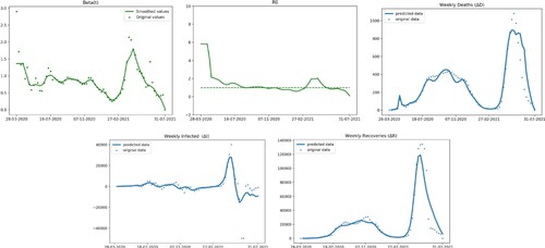
4.3. Graphical analysis of βstates/UT of India

In our work, instead of providing graphs for 13 parameters, we have selected 5 important parameters (${\beta }_i$, $R_0$, $\mathrm{\Delta }D$, $\mathrm{\Delta }I$, and $\mathrm{\Delta }R$) to reduce the size of the article. The Figures 2–36 demonstrates the graphical analysis of ${\beta }_i$, $R_0$, $\mathrm{\Delta }D$, $\mathrm{\Delta }I$, and $\mathrm{\Delta }R$ for all States/UT of India.

Figure 1. Compartments of the SIRD Model.

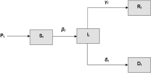
Figure 2. Graphical analysis of ${\beta }_i$, $R_0$, $\mathrm{\Delta }D$, $\mathrm{\Delta }I$, and $\mathrm{\Delta }R$ for Andaman & Nicobar Islands.

Figure 3. Graphical analysis of ${\beta }_i$, $R_0$, $\mathrm{\Delta }D$, $\mathrm{\Delta }I$, and $\mathrm{\Delta }R$ of Andhra Pradesh.

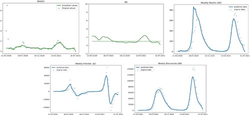
Figure 4. Graphical analysis of ${\beta }_i$, $R_0$, $\mathrm{\Delta }D$, $\mathrm{\Delta }I$, and $\mathrm{\Delta }R$ of Arunachal Pradesh.

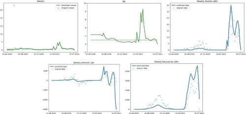
Figure 5. Graphical analysis of ${\beta }_i$, $R_0$, $\mathrm{\Delta }D$, $\mathrm{\Delta }I$, and $\mathrm{\Delta }R$ of Assam.

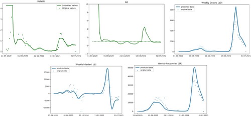
Figure 6. Graphical analysis of ${\beta }_i$, $R_0$, $\mathrm{\Delta }D$, $\mathrm{\Delta }I$, and $\mathrm{\Delta }R$ of Bihar.

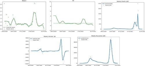
Figure 7. Graphical analysis of ${\beta }_i$, $R_0$, $\mathrm{\Delta }D$, $\mathrm{\Delta }I$, and $\mathrm{\Delta }R$ of Chandigarh.

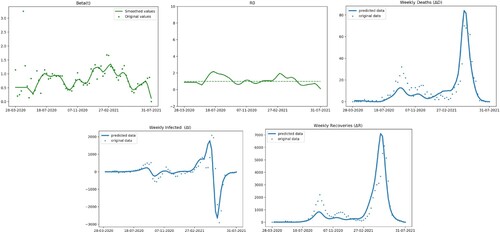
Figure 8. Graphical analysis of ${\beta }_i$, $R_0$, $\mathrm{\Delta }D$, $\mathrm{\Delta }I$, and $\mathrm{\Delta }R$ of Chhattisgarh.

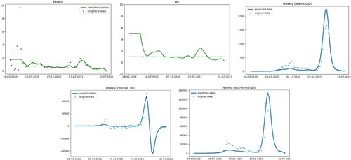
Figure 9. Graphical analysis of ${\beta }_i$, $R_0$, $\mathrm{\Delta }D$, $\mathrm{\Delta }I$, and $\mathrm{\Delta }R$ of Dadra & Nagar Haveli and Daman & Diu.

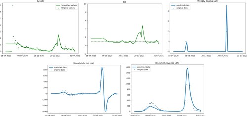
Figure 10. Graphical analysis of ${\beta }_i$, $R_0$, $\mathrm{\Delta }D$, $\mathrm{\Delta }I$, and $\mathrm{\Delta }R$ of Delhi.

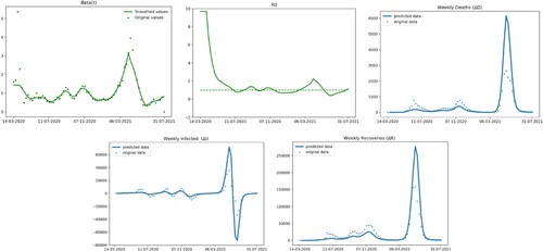
Figure 11. Graphical analysis of ${\beta }_i$, $R_0$, $\mathrm{\Delta }D$, $\mathrm{\Delta }I$, and $\mathrm{\Delta }R$ of Goa.

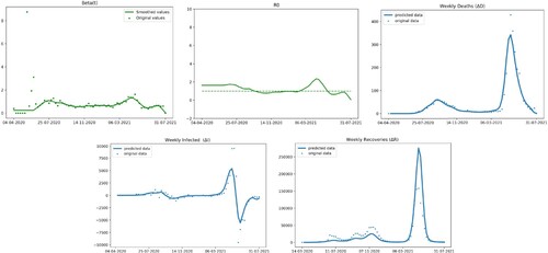
Figure 12. Graphical analysis of ${\beta }_i$, $R_0$, $\mathrm{\Delta }D$, $\mathrm{\Delta }I$, and $\mathrm{\Delta }R$ of Gujarat.

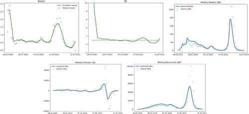
Figure 13. Graphical analysis of ${\beta }_i$, $R_0$, $\mathrm{\Delta }D$, $\mathrm{\Delta }I$, and $\mathrm{\Delta }R$ of Haryana.

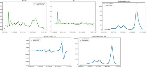
Figure 14. Graphical analysis of ${\beta }_i$, $R_0$, $\mathrm{\Delta }D$, $\mathrm{\Delta }I$, and $\mathrm{\Delta }R$ of Himachal Pradesh.

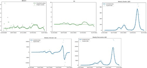
Figure 15. Graphical analysis of ${\beta }_i$, $R_0$, $\mathrm{\Delta }D$, $\mathrm{\Delta }I$, and $\mathrm{\Delta }R$ of Jammu and Kashmir.

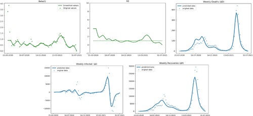
Figure 16. Graphical analysis of ${\beta }_i$, $R_0$, $\mathrm{\Delta }D$, $\mathrm{\Delta }I$, and $\mathrm{\Delta }R$ of Jharkhand.

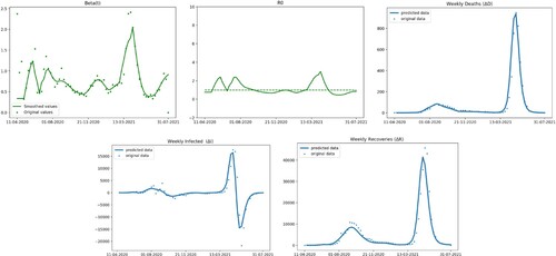
Figure 17. Graphical analysis of ${\beta }_i$, $R_0$, $\mathrm{\Delta }D$, $\mathrm{\Delta }I$, and $\mathrm{\Delta }R$ of Karnataka.

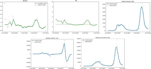
Figure 18. Graphical analysis of ${\beta }_i$, $R_0$, $\mathrm{\Delta }D$, $\mathrm{\Delta }I$, and $\mathrm{\Delta }R$ of Kerala.

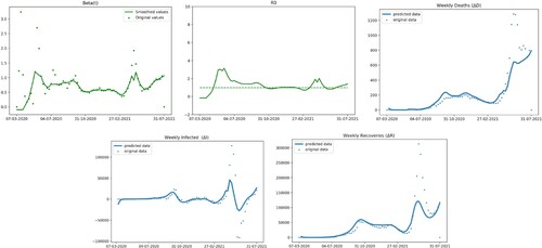
Figure 19. Graphical analysis of ${\beta }_i$, $R_0$, $\mathrm{\Delta }D$, $\mathrm{\Delta }I$, and $\mathrm{\Delta }R$ of Ladakh.

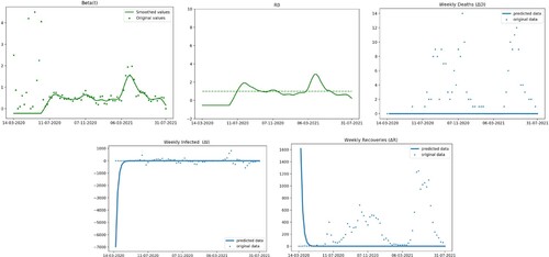
Figure 20. Graphical analysis of ${\beta }_i$, $R_0$, $\mathrm{\Delta }D$, $\mathrm{\Delta }I$, and $\mathrm{\Delta }R$ of Madhya Pradesh.

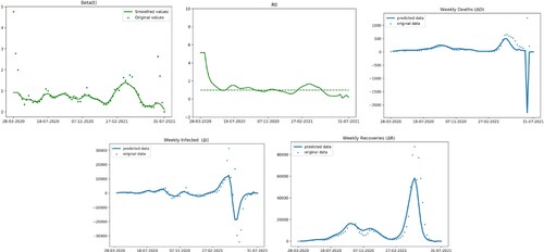
Figure 21. Graphical analysis of ${\beta }_i$, $R_0$, $\mathrm{\Delta }D$, $\mathrm{\Delta }I$, and $\mathrm{\Delta }R$ of Maharashtra.

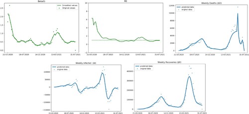
Figure 22. Graphical analysis of ${\beta }_i$, $R_0$, $\mathrm{\Delta }D$, $\mathrm{\Delta }I$, and $\mathrm{\Delta }R$ of Manipur.

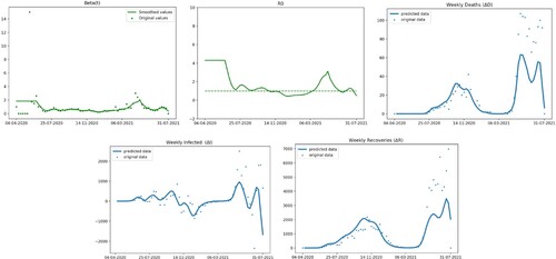
Figure 23. Graphical analysis of ${\beta }_i$, $R_0$, $\mathrm{\Delta }D$, $\mathrm{\Delta }I$, and $\mathrm{\Delta }R$ of Meghalaya.

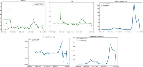
Figure 24. Graphical analysis of ${\beta }_i$, $R_0$, $\mathrm{\Delta }D$, $\mathrm{\Delta }I$, and $\mathrm{\Delta }R$ of Mizoram.

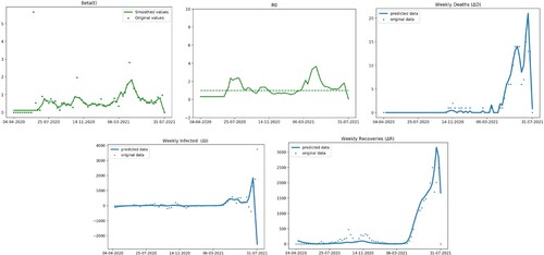
Figure 25. Graphical analysis of ${\beta }_i$, $R_0$, $\mathrm{\Delta }D$, $\mathrm{\Delta }I$, and $\mathrm{\Delta }R$ of Nagaland.

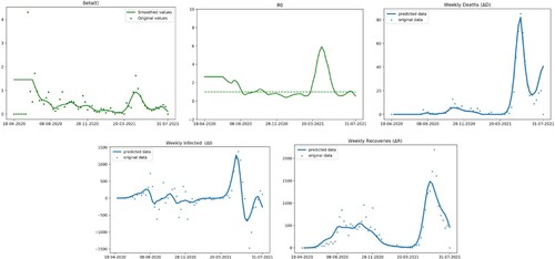
Figure 26. Graphical analysis of ${\beta }_i$, $R_0$, $\mathrm{\Delta }D$, $\mathrm{\Delta }I$, and $\mathrm{\Delta }R$ of Odisha.

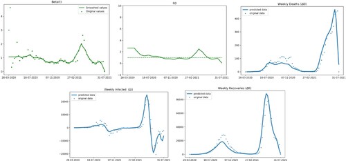
Figure 27. Graphical analysis of ${\beta }_i$, $R_0$, $\mathrm{\Delta }D$, $\mathrm{\Delta }I$, and $\mathrm{\Delta }R$ of Puducherry.

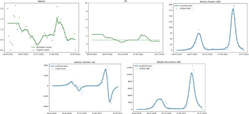
Figure 28. Graphical analysis of ${\beta }_i$, $R_0$, $\mathrm{\Delta }D$, $\mathrm{\Delta }I$, and $\mathrm{\Delta }R$ of Punjab.

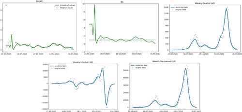
Figure 29. Graphical analysis of ${\beta }_i$, $R_0$, $\mathrm{\Delta }D$, $\mathrm{\Delta }I$, and $\mathrm{\Delta }R$ of Rajasthan.

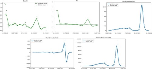
Figure 30. Graphical analysis of ${\beta }_i$, $R_0$, $\mathrm{\Delta }D$, $\mathrm{\Delta }I$, and $\mathrm{\Delta }R$ of Sikkim.

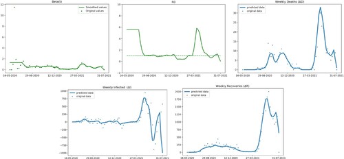
Figure 31. Graphical analysis of ${\beta }_i$, $R_0$, $\mathrm{\Delta }D$, $\mathrm{\Delta }I$, and $\mathrm{\Delta }R$ of Tamil Nadu.

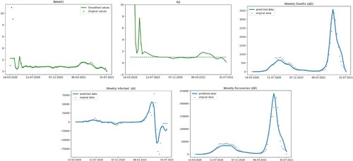
Figure 32. Graphical analysis of ${\beta }_i$, $R_0$, $\mathrm{\Delta }D$, $\mathrm{\Delta }I$, and $\mathrm{\Delta }R$ of Telangana.

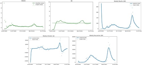
Figure 33. Graphical analysis of ${\beta }_i$, $R_0$, $\mathrm{\Delta }D$, $\mathrm{\Delta }I$, and $\mathrm{\Delta }R$ of Tripura.

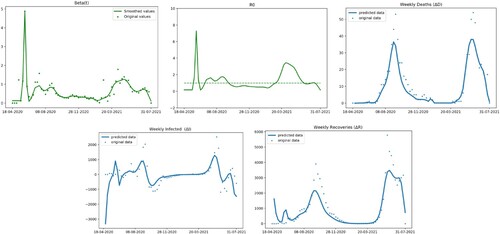
Figure 34. Graphical analysis of ${\beta }_i$, $R_0$, $\mathrm{\Delta }D$, $\mathrm{\Delta }I$, and $\mathrm{\Delta }R$ of Uttarakhand.

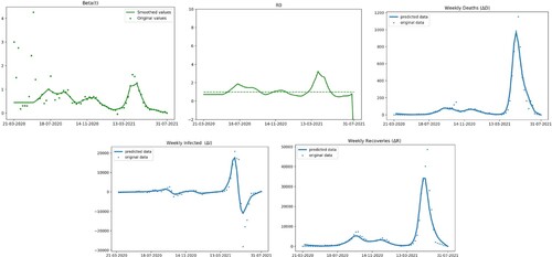
Figure 35. Graphical analysis of ${\beta }_i$, $R_0$, $\mathrm{\Delta }D$, $\mathrm{\Delta }I$, and $\mathrm{\Delta }R$ of Uttar Pradesh.

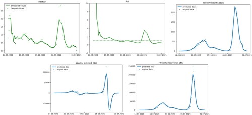
Figure 36. Graphical analysis of ${\beta }_i$, $R_0$, $\mathrm{\Delta }D$, $\mathrm{\Delta }I$, and $\mathrm{\Delta }R$ of West Bengal.

From the graphs we observe that:

1. Andaman and Nicobar Islands: In Andaman & Nicobar Islands, over time, the transmission coefficient decreased, signalling a decline in COVID-19 cases. This decrease in transmission was reflected in a drop in the reproductive number and a reduction in weekly deaths. However, despite this decline, the number of new infections remained high, leading to a lower recovery rate among individuals infected on a weekly basis.

2. Andhra Pradesh: In Andhra Pradesh, there has been a gradual reduction in the transmission coefficient, indicating a decline in COVID-19 cases. This decrease in transmission has corresponded to a decrease in the reproductive number and a reduction in weekly fatalities. Nevertheless, despite this decline, the volume of new infections has persisted at a high level, resulting in a lower recovery rate for individuals contracting the virus on a weekly basis.

3. Arunachal Pradesh: In Arunachal Pradesh, as time progressed, the transmission coefficient decreased, leading to a decline in the reproductive number. Although the number of weekly deaths remained constant, there was a decrease in the weekly infected individuals and weekly recoveries.

4. Assam: In Assam, with time, the decreasing transmission coefficient resulted in a decline in the reproductive number. Despite a rise in weekly deaths, there was no alteration in the number of weekly infected individuals, while weekly recoveries experienced a decrease.

5. Bihar, Chandigarh, and Chhatisgarh: In Bihar, Chandigarh, and Chattisgarh, a decrease in the transmission coefficient led to a lower reproductive number, indicating a decrease in COVID-19 cases. However, there was an observed increase in weekly deaths, a rise in the number of weekly infected individuals, and a decrease in weekly recoveries.

6. Dadra & Nagar Haveli and Daman & Diu: In Dadra & Nagar Haveli and Daman & Diu, the drop in the transmission coefficient caused a decrease in the reproductive number. Weekly deaths stayed steady while the number of infected individuals increased, and weekly recoveries declined.

7. Delhi: In Delhi, there was a decrease in the transmission coefficient, while the reproductive number remained steady over time. Weekly deaths rose, while the numbers of weekly infected individuals and weekly recoveries remained consistent.

8. Goa: In Goa, a drop in the transmission coefficient resulted in a reduced reproductive number, signalling a decline in COVID-19 cases. Yet, there was an increase in weekly deaths, an increase in newly infected individuals on a weekly basis, and a decline in weekly recoveries.

9. Gujrat: In Gujrat, the transmission coefficient decreased while the reproductive number increased. However, this shift coincided with a rise in weekly deaths, an escalation in new weekly infections, and a drop in weekly recoveries.

10. Haryana, Himachal Pradesh, and Jammu & Kashmir: In Haryana, Himachal Pradesh, and Jammu & Kashmir, a drop in the transmission coefficient resulted in a reduced reproductive number, signalling a decline in COVID-19 cases. Nonetheless, there was a noted rise in weekly deaths, an escalation in the count of weekly infections, and a decline in weekly recoveries.

11. Jharkhand, Karnataka, and Kerala: Over time in Jharkhand, Karnataka, and Kerala, there was a gradual decrease in the transmission coefficient and a simultaneous increase in the reproductive number. This shift coincided with an increase in weekly deaths and newly infected individuals, alongside a decline in weekly recoveries.

12. Ladakh, Madhya Pradesh, Maharashtra, and Manipur: A decline in the reproductive number in Ladakh, Madhya Pradesh, Maharashtra, and Manipur was accompanied by a fall in the transmission coefficient, which suggested a decline in COVID-19 cases. However, there was a weekly rise in the number of infected patients, a weekly drop in recoveries, and a weekly increase in deaths.

13. Meghalaya, Mizoram, Nagaland, and Tripura: The decrease in the reproductive number in Meghalaya, Mizoram, Nagaland, and Tripura corresponded with a reduction in the transmission coefficient, indicating a decrease in COVID-19 cases. This was accompanied by a weekly decrease in the count of infected patients, a decline in weekly recoveries, and a weekly rise in deaths.

14. Odisha, Puducherry, and Punjab: A decrease in the reproductive number in Odisha, Puducherry, and Punjab, along with a dip in the transmission coefficient, indicated a decrease in COVID-19 cases. However, there was a noticeable increase in weekly fatalities, a rise in weekly infections, and a decrease in weekly recoveries.

15. Rajasthan and Telangana: In Rajasthan and Telangana, there was a gradual decrease in the transmission coefficient alongside a rise in the reproductive number. This coincided with an increase in weekly deaths and newly infected individuals, coupled with a decline in weekly recoveries.

16. Sikkim and Tamil Nadu: In Sikkim and Tamil Nadu, the number of reproductive individuals declined concurrently with a decline in the transmission coefficient. On the other hand, weekly infections increased, weekly recoveries decreased, and weekly mortality clearly increased.

17. Uttar Pradesh, Uttarakhand, and West Bengal: Reduced reproductive numbers in Uttar Pradesh, Uttarakhand, and West Bengal are indicative of a decline in COVID-19 cases, as evident by declining transmission coefficient. But there was also a weekly rise in the number of infected people, a weekly decline in recoveries, and an observed increase in weekly deaths.

Table 6 illustrates the comparison between the actual and predicted values of confirmed, recovered and deceased cases for all States/UTs of India.

Table 6. Comparative analysis of actual predicted values of confirmed, recovered, and deceased cases for all States/UT of India.

S.No	Name of State/UT	Confirmed	Predicted Confirmed	Recovered	Predicted Recovered	Deceased	Predicted Deceased
1.	Andman and Nichobar Islands	7532	7478	7392	7320	129	156
2.	Andhra Pradesh	1,960,196	1,769,605	1,925,521	1,749,236	13,313	14,253
3.	Arunachal Pradesh	47,088	51,516	42,648	49,568	222	262
4.	Assam	562,590	5,731,379	542,963	5,738,581	5200	6560
5.	Bihar	724,659	684,612	714,542	677,247	9640	7357
6.	Chandigarh	61,941	62,389	61,097	61,630	809	757
7.	Chhattisgarh	1,001,622	1,006,249	985,847	989,578	13,519	15,157
8.	Dadra and Nagar Haveli & Daman and Diu	10,644	11,030	10,569	10,840	4	6
9.	Delhi	1436,084	1,616,702	1,410,469	1,581,602	25,048	33,730
10.	Goa	170,815	160,254	166,569	156,916	3141	3041
11.	Gujarat	824,798	695,092	814,439	685,086	10,076	9034
12.	Haryana	769,826	704,621	759,490	694,408	9627	9193
13.	Himachal Pradesh	205,538	183,669	201,229	180,304	3502	3242
14.	Jammu and Kashmir	321,045	286,261	315,492	281,822	4376	4309
15.	Jharkhand	347,059	334,411	341,682	328,721	5125	5388
16.	Karnataka	2,899,583	2,801,593	2,839,944	2,732,819	36,464	37,574
17.	Kerala	3,328,207	2,915,371	3,160,959	2,746,482	16,436	14,905
18.	Ladakh	20,319	7021	20,049	7021	207	0
19.	Madhya Pradesh	791,783	680,819	781,137	675,021	10,512	5802
20.	Maharashtra	6,283,474	5,883,174	6,064,962	5,601,583	132,121	124,855
21.	Manipur	95,712	68,638	83,485	64,827	1513	1031
22.	Meghalaya	63,071	56,874	56,536	54,823	1051	1077
23.	Mizoram	35,290	30,897	24,808	26,538	140	150
24.	Nagaland	27,566	27,666	24,938	24,648	553	637
25.	Odisha	972,450	972,940	951,114	965,564	5756	5512
26.	Puducherry	120,622	115,122	117,889	112,724	1791	1778
27.	Punjab	598,946	575,497	582,075	559,826	16,283	15,574
28.	Rajasthan	953,603	883,181	944,376	873,921	8952	8849
29.	Sikkim	25,851	24,235	22,080	22,239	335	344
30.	Tamil Nadu	2,553,929	2,591,283	2,498,122	2,538,980	33,994	35,750
31.	Telangana	643,067	614,851	630,034	598,333	3793	5743
32.	Tripura	77,350	67,939	72,824	66,264	745	603
33.	Uttar Pradesh	1,708,304	1,612,006	1,684,762	1,586,990	22,753	24,086
34.	Uttarakhand	341,922	333,837	327,880	306,886	7360	7367
35.	West Bengal	1,525,782	1,525,458	1,496,289	1,491,219	18,107	19,215

5. Conclusion

This paper introduces a modified hybrid SIRD model designed to assess the impact of diverse government interventions aimed at curbing the spread of COVID-19 in India. The utilization of the Modified Grey Wolf Optimizer helps determine the optimal initial value for Infected individuals, improving predictions based on reported data. To minimize Process and Measurement Noise, the LOWESS smoothing function is employed. The model is applied to weekly data spanning from 30 January 2020 to 31 July 2021, and post this period, arrows are used to project the COVID-19 trend for a brief duration. The graphical analysis, considering transmission coefficient, reproductive number, weekly deaths, weekly infected, and weekly recovered, indicates a decline in the COVID-19 pandemic across most States/Union Territories of India, barring a few such as Gujarat, Jharkhand, Karnataka, Kerala, Rajasthan, and Telangana, where an upward trend is observed. Delhi, however, demonstrates a stable COVID-19 trend. Notably, the analysis closely aligns with actual/reported values. This modified hybrid SIRD model holds potential for further exploration into the post-vaccination impact of COVID-19 in India and other countries. Additionally, it stands as a valuable tool for government authorities and researchers in predicting short-term trends post-31 July 2021.

Authors' contributions

The authors contributed equally and significantly in writing this paper. All authors read and approved the final manuscript.

Disclosure statement

There is no conflict of interest regarding the publication of this article.

Data availability statement

We used data from the link – https://www.covid19india.org/ to support this study.

References

- World Health Organization. Coronavirus overview. Available from: https://www.who.int/health-topics/coronavirus
- Brauer F. Compartmental models in epidemiology. In: Fred Brauer editor. Mathematical epidemiology. Vancouver (BC): Department of Mathematics, University of British Columbia; 2008. p. 19–79.
- Kermack WO, McKendrick AG. A contribution to the mathematical theory of epidemics. Proc R Soc Lond Ser A-Contain Pap Math Phys Character. 1927;115(772):700–721.
- Saha S, Dutta P, Samanta G. Dynamical behavior of sirs model incorporating government action and public response in presence of deterministic and fluctuating environments. Chaos, Solitons & Fractals. 2022;164:112643. doi: 10.1016/j.chaos.2022.112643
- Ross R. An application of the theory of probabilities to the study of a priori pathometry – Part I. Proc R Soc Lond Ser A-Contain Pap Math Phys Character. 1916;92(638):204–230.
- Caccavo D. Chinese and Italian Covid-19 outbreaks can be correctly described by a modified SIRD model. medRxiv; 2020.
- Calafiore GC, Novara C, Possieri C. A time-varying SIRD model for the Covid-19 contagion in Italy. Annu Rev Control. 2020;50:361–372.
- Sen D, Sen D. Use of a modified SIRD model to analyze Covid-19 data. Ind Eng Chem Res. 2021;60(11):4251–4260. doi: 10.1021/acs.iecr.0c04754
- Khajanchi S, Sarkar K, Mondal J, et al. Mathematical modeling of the Covid-19 pandemic with intervention strategies. Results Phys. 2021;25:104285. doi: 10.1016/j.rinp.2021.104285
- Rai RK, Khajanchi S, Tiwari PK, et al. Impact of social media advertisements on the transmission dynamics of Covid-19 pandemic in India. J Appl Math Comput. 2022;68:1–26.
- Samui P, Mondal J, Khajanchi S. A mathematical model for Covid-19 transmission dynamics with a case study of India. Chaos, Solitons & Fractals. 2020;140:110173. doi: 10.1016/j.chaos.2020.110173
- Khajanchi S, Sarkar K. Forecasting the daily and cumulative number of cases for the Covid-19 pandemic in India. Chaos: Interdis J Nonlinear Sci. 2020;30(7):071101. doi: 10.1063/5.0016240
- Sarkar K, Khajanchi S, Nieto JJ. Modeling and forecasting the Covid-19 pandemic in India. Chaos, Solitons & Fractals. 2020;139:110049. doi: 10.1016/j.chaos.2020.110049
- Khajanchi S, Sarkar K, Mondal J. Dynamics of the Covid-19 pandemic in India; 2020. arXiv preprint arXiv:2005.06286.
- Ghosh S, Samanta GP, Mubayi A. Comparison of regression approaches for analyzing survival data in the presence of competing risks. Lett Biomath. 2021;8(1):29–47.
- Ghosh S, Samanta G, Nieto JJ. Application of non-parametric models for analyzing survival data of Covid-19 patients. J Infect Public Health. 2021;14(10):1328–1333. doi: 10.1016/j.jiph.2021.08.025
- Saha S, Samanta GP, Nieto JJ. Epidemic model of Covid-19 outbreak by inducing behavioural response in population. Nonlinear Dyn. 2020;102:455–487. doi: 10.1007/s11071-020-05896-w
- Mondal J, Khajanchi S. Mathematical modeling and optimal intervention strategies of the Covid-19 outbreak. Nonlinear Dyn. 2022;109(1):177–202. doi: 10.1007/s11071-022-07235-7
- Tiwari PK, Rai RK, Khajanchi S, et al. Dynamics of coronavirus pandemic: effects of community awareness and global information campaigns. Eur Phys J Plus. 2021;136(10):994. doi: 10.1140/epjp/s13360-021-01997-6
- Shringi S, Sharma H, Rathie PN, et al. Modified SIRD model for Covid-19 spread prediction for northern and southern states of india. Chaos, Solitons & Fractals. 2021;148:111039. doi: 10.1016/j.chaos.2021.111039
- Van Doremalen N, Bushmaker T, Morris DH, et al. Aerosol and surface stability of SARS-COV-2 as compared with SARS-COV-1. N Engl J Med. 2020;382(16):1564–1567. doi: 10.1056/NEJMc2004973
- Mirjalili S, Mirjalili SM, Lewis A. Grey wolf optimizer. Adv Eng Softw. 2014;69:46–61. doi: 10.1016/j.advengsoft.2013.12.007
- Worldometer. India population (2020); 2020; [cited 2020 Oct 24]. Available from: https://www.worldometers.info/world-population/
- Liu Y, Gayle AA, Wilder-Smith A, et al. The reproductive number of Covid-19 is higher compared to sars coronavirus. J Travel Med. 2020;27(2):1–4.
- UN News. Covid-19: lockdown across india, in line with who guidance [Internet]. March 24, 2020; [cited 2020 Oct 25]. Available from: https://news.un.org/en/story/2020/03/1060132
- NDTV. Lockdown for 2 more weeks starting 4th may. Available from: https://www.ndtv.com/india
- The Tribune. Centre extends nationwide lockdown till May 31, new guidelines issued. Thursday, February 9, 2023; [cited 2020 Oct 25]. Available from: https://www.tribuneindia.com/news/nation/centre-extends-nationwide-lockdown-till-may-31-new-guidelines-issued-86042
- Deepshikha (ed.). Sharma, Neeta (30 May 2020). Ghosh. ‘Unlock1: malls, restaurants, places of worship to reopen June 8’. NDTV. Retrieved 30 may 2020. (accessed on 25/10/2020).
- Deeptiman (30 June 2020). Tiwary. ‘Unlock 2: more flights, trains, but no schools and colleges till July 31’. The Indian Express. Retrieved 1 July 2020. (accessed on 25/10/2020).
- What's not. The Indian Express, July 30, 2020. Retrieved 1 August 2020. ‘Unlock 3.0 guidelines: here is what's allowed. (accessed on 25/10/2020).
- The Indian Express. Retrieved 2 September 2020. ‘Unlock 4.0: full guidelines issued by different states’. (accessed on 25/10/2020).
- Social gatherings. ‘Unlock 5.0 guidelines explained: what are the rules for schools and 2020. Cinemas?’ The Indian Express. Retrieved 1 October. (accessed on 25/10/2020).
- COVID 19 INDIA. Dataset. [cited 2020 Oct 24]. Available from: https://www.covid19india.org/
- Pintus E, Sorbolini S, Albera A, et al. Use of locally weighted scatterplot smoothing (lowess) regression to study selection signatures in Piedmontese and Italian Brown cattle breeds. Anim Genet. 2014;45(1):1–11. doi: 10.1111/age.2013.45.issue-1
- Yang X-S. Nature-inspired metaheuristic algorithms. United Kingdom: Luniver Press; 2010.
- Talbi E-G. Metaheuristics: from design to implementation. Hoboken, New Jersey: John Wiley & Sons; 2009.
- Nesmachnow S. An overview of metaheuristics: accurate and efficient methods for optimisation. Int J Metaheuristics. 2014;3(4):320–347. doi: 10.1504/IJMHEUR.2014.068914
- The Hindu. India's first coronavirus infection confirmed in Kerala; 2020. Available from: https://www.thehindu.com/news/national/indias-first-coronavirus-infection-confirmed-in-kerala/article30691004.ece
- Khajanchi S, Bera S, Roy TK. Mathematical analysis of the global dynamics of a HTLV-I infection model, considering the role of cytotoxic T-lymphocytes. Math Comput Simul. 2021;180:354–378. doi: 10.1016/j.matcom.2020.09.009