A modified projective forward-backward splitting algorithm for variational inclusion problems to predict Parkinson's disease

Abstract

This research studies variational inclusion problems, which is a branch of optimization. A modified projective forward-backward splitting algorithm is constructed to solve this problem. The algorithm adds the inertial technique for speeding up the convergence, and the projective method for several regularization machine learning models to meet good model fitting. To evaluate the performance of the classification models employed in this research, four evaluation metrics are computed: accuracy, F1-score, recall, and precision. The highest performance value of 92.86% accuracy, 62.50% precision, 100% recall, and 76.92% F1-score shows that our algorithm performs better than the other machine learning models.

Keywords:

• Variational inclusion problem
• extreme learning machines (ELM)
• forward-backward splitting algorithm
• regularized least squares
• Parkinson's disease

Mathematics Subject Classifications:

• 46T99
• 47H04
• 47J25
• 49M25

1. Introduction

The variational inclusion problem (VIP) is to find a point ${\omega }^{\ast }$ in a real Hilbert space $\mathbf{H}$ such that (1) $0\in (\mathbb{F}+\mathbb{G}){\omega }^{\ast },$(1) where $\mathbb{F}:\mathbf{H}\to \mathbf{H}$ is a single valued mapping and $\mathbb{G}:\mathbf{H}\to 2^{\mathbf{H}}$ is a multivalued mapping. Solving the VIP (1(1) $0\in (\mathbb{F}+\mathbb{G}){\omega }^{\ast },$(1) ) has many benefits for specific applications since many problems can be formulated in the form of the VIP (1(1) $0\in (\mathbb{F}+\mathbb{G}){\omega }^{\ast },$(1) ), such as minimization problems, machine learning, image processing, signal processing, etc., see in [1–3]. This paper focuses on modifying efficient algorithms to solve the VIP (1(1) $0\in (\mathbb{F}+\mathbb{G}){\omega }^{\ast },$(1) ) and applying them to decrypt data classification. The inertial extrapolation technique, which was introduced in 1964, is one of the techniques for ensuring the algorithm's good convergence [4]. The main feature of the inertia extrapolation technique is that the next iterate is constructed by the previous two iterates. This technique was used extensively with variational inclusion algorithms later by many authors, see in [5–9]. The inertial forward-backward algorithm (IFB) is the original variational inclusion algorithm introduced by Moudafi and Oliny [10]. The algorithm was generated by ${\omega }^0,{\omega }^1\in \mathbf{H}$ and (2) $\begin{array}{rl}{y}^k& ={\omega }^k+{\sigma }^k({\omega }^k-{\omega }^{k-1}),\\ {\omega }^{k+1}& =J_{{\tau }^k}^{\mathbb{G}}(y^k-{\tau }^k\mathbb{F}{\omega }^k),k\ge 0,\end{array}$(2) where $\left\{{\tau }^k\right\}$ is a sequence of positive real numbers. The weak convergence of the iterative sequence was established based on the condition generated in terms of the sequence $\left\{{\omega }^k\right\}$ and parameter ${\sigma }^k$ under a co-coercivity condition $\mathbb{F}$ about the solution set. Following the idea of Moudafi and Oliny [10], Peeyada et al. [11] introduced an inertial Mann forward-backward splitting algorithm (IMFB) for the VIP (1(1) $0\in (\mathbb{F}+\mathbb{G}){\omega }^{\ast },$(1) ) by taking ${\omega }^0,{\omega }^1\in \mathbf{H}$ and (3) $\begin{array}{rl}{y}^k& ={\omega }^k+{\sigma }^k({\omega }^k-{\omega }^{k-1}),\\ z^k& =y^k+{\alpha }^k({\omega }^k-y^k),\\ {\omega }^{k+1}& =J_{{\tau }^k}^{\mathbb{G}}(z^k-{\tau }^k\mathbb{F}{z}^k),k\ge 0,\end{array}$(3) where $\left\{{\tau }^k\right\}$ is a sequence of positive real numbers and $\left\{{\alpha }^k\right\}\subset [0,1]$. Under the same conditions on a co-coercivity condition $\mathbb{F}$, the parameters ${\alpha }^k,{\tau }^k$, and $\sum _{k=1}^{\mathrm{\infty }}{\sigma }^k\Vert {\omega }^k-{\omega }^{k-1}\Vert <\mathrm{\infty }$, weak convergence of algorithm was proved. The IMFB was used in machine learning for breast cancer classification, and its efficiency was presented by comparing it with other algorithms. The regularized least square model was solved by setting the VIP (1(1) $0\in (\mathbb{F}+\mathbb{G}){\omega }^{\ast },$(1) ) for getting an optimal fitting model in machine learning, thus the IMFB is very useful for breast cancer classification. Many optimization branches have been used in various neural networks and medical fields in recent years [12–16]. Parkinson's disease is a gradual degenerative disease of the brain that is common in the elderly. There is currently no cure for this disease, although early detection and treatment by a medical practitioner can help reduce the progression of the disease and improve the quality of life. Many machine learning methods such as Bayesian optimization (BO), Support Vector Machine (SVM), Random Forest (RF), Logistic Regression (LR), etc. (see in [17]) have been used for Parkinson's disease detection. The extreme learning machine (ELM) is also used in Parkinson's disease detection (see in [18]), with the aid of the feature selection techniques the method got an efficient model.

To solve the VIP (1(1) $0\in (\mathbb{F}+\mathbb{G}){\omega }^{\ast },$(1) ), we present a modified inertial two-step Mann forward-backward splitting algorithm with projective methods inspired by prior research. Weak convergence is demonstrated under appropriate conditions to confirm solution convergence. In the final section, we show how our algorithm can be used to Parkinson's disease detection by the ELM without data cleaning technique and compare it to various machine learning methods.

2. Preliminaries

In this section, we provide various definitions and lemmas that will be needed to prove our optimization algorithm in Section 3. We use the symbols $\rightharpoonup$ and $\to$ to denote weak and strong convergence, respectively.

Definition 2.1

$\mathbb{F}:\mathbf{H}\to \mathbf{H}$ is called $\mathbf{L}$-Lipschitz continuous if there exists $\mathbf{L}>0$ such that $\Vert \mathbb{F}\omega -\mathbb{F}\nu \Vert \le \mathbf{L}\Vert \omega -\nu \Vert$ for all $\omega ,\nu \in \mathbf{H}$. $\mathbb{F}$ is nonexpansive mapping for $\mathbf{L}=1$.

Definition 2.2

Assume that $\mathbb{G}:\mathbf{H}\to 2^{\mathbf{H}}$ is a multivalued mapping and its graph mapping is denoted by $\mathrm{graph}\left(\mathbb{G}\right)$. $\mathbb{G}$ is called

(i)	monotone if ∀$(\omega ,u),(\nu ,v)\in \mathrm{graph}\left(\mathbb{G}\right)$, $〈u-v,\omega -\nu 〉\ge 0,$
(ii)	maximal monotone if ∀$(\omega ,u)\in \mathbf{H}\times \mathbf{H}$, $〈u-v,\omega -\nu 〉\ge 0$ ∀$(\nu ,v)\in \mathrm{graph}\left(\mathbb{G}\right)$⇔$(\omega ,u)\in \mathrm{graph}\left(\mathbb{G}\right)$.
(iii)	α-inverse strongly monotone if ∃$\alpha >0$ such that $〈\mathbb{G}x-\mathbb{G}y,x-y〉\ge \alpha \Vert \mathbb{G}x-\mathbb{G}y{\Vert }^2$ ∀$x,y\in \mathcal{H}$.

Lemma 2.3

[19]

Assume $\mathbb{F}:\mathbf{H}\to \mathbf{H}$ is a mapping and that $\mathbb{G}:\mathbf{H}\to 2^{\mathbf{H}}$ is a maximal monotone mapping. Let $T_{\tau }:=(I+\tau \mathbb{G}{)}^{-1}(I-\tau \mathbb{F})$, $\tau >0$, and $\mathrm{Fix}\left(T_{\tau }\right)$ be the set of the fixed points of $T_{\tau }$. Then $\mathrm{Fix}\left(T_{\tau }\right)=(\mathbb{F}+\mathbb{G}{)}^{-1}(0)$.

Lemma 2.4

[20]

Assume $\mathbb{G}:\mathbf{H}\to 2^{\mathbf{H}}$ is a maximal monotone mapping and that $\mathbb{F}:\mathbf{H}\to \mathbf{H}$ is a Lipschitz continuous and monotone mapping. Then the mapping $\mathbb{F}+\mathbb{G}$ is maximal monotone.

Lemma 2.5

[21]

Assume $\mathbb{F}:\mathbf{H}\to \mathbf{H}$ is α-inverse-strongly monotone mapping. Then

1. $\mathbb{F}$ is $\frac{1}{\alpha }$-Lipschitz continuous and monotone.

2. If $\tau \in (0,2\alpha ]$ is a constant, then $I-\tau \mathbb{F}$ is nonexpansive, where I is the identity mapping on $\mathbf{H}$.

Lemma 2.6

[22]

Assume $\mathbb{F}:\mathbf{H}\to \mathbf{H}$ is a α-inverse-strongly monotone mapping and that $\mathbb{G}:\mathbf{H}\to 2^{\mathbf{H}}$ is maximal monotone mapping. Then

1. For $\tau >0$, $\mathrm{Fix}\left(J_{\tau }^{\mathbb{G}}\right(I-\tau \mathbb{F}\left)\right)=(\mathbb{F}+\mathbb{G}{)}^{-1}(0)$,

2. For $0<\tau \le \overline{\tau }$ and $x\in \mathbf{H}$, $\Vert x-J_{\tau }^{\mathbb{G}}(I-\tau \mathbb{F})x\Vert \le 2\Vert x-J_{\overline{\tau }}^{\mathbb{G}}(I-\overline{\tau }\mathbb{F})x\Vert$.

Lemma 2.7

[23]

Assume $\mathbb{F}:\mathbf{H}\to \mathbf{H}$ is a nonexpansive mapping with $\mathrm{Fix}\left(\mathbb{F}\right)\ne \mathrm{\varnothing }$. If there exists a sequence $\left\{{\omega }^k\right\}$ in $\mathbf{H}$ with ${\omega }^k\rightharpoonup \omega \in \mathbf{H}$ and $\Vert {\omega }^k-\mathbb{F}{\omega }^k\Vert \to 0$, then $\omega \in \mathrm{Fix}\left(\mathbb{F}\right)$.

Lemma 2.8

[24]

Assume that $\left\{{\alpha }^k\right\}$ and $\left\{{\text{β}}^k\right\}$ are nonnegative real sequences with $\sum _{n=1}^{\mathrm{\infty }}{\text{β}}^k<\mathrm{\infty }$ and ${\alpha }^{k+1}\le {\alpha }^k+{\text{β}}^k.$ Then, $\left\{{\alpha }^k\right\}$ is convergent.

Lemma 2.9

[19, Opial]

Assume that $\mathbf{C}$ is a nonempty set of $\mathbf{H}$ and $\left\{{\omega }^k\right\}$ is a sequence in $\mathbf{H}$. Assume that the following are true.

1. $\{\Vert {\omega }^k-\omega \Vert \}$ converges, ∀$\omega \in \mathbf{C}$.

2. Every weak sequential cluster point of $\left\{{\omega }^k\right\}$ is in $\mathbf{C}$.

   Then $\left\{{\omega }^k\right\}$ converges weakly to a point in $\mathbf{C}$.

3. Optimization algorithm

The section aims to present the convergence analysis. Let $\mathbf{C}$ be a nonempty closed convex subset of a real Hilbert space $\mathbf{H}$, and consider the following conditions.

(C1)	$\mathbb{G}:\mathbf{H}\to 2^{\mathbf{H}}$ is maximal monotone mapping.
(C2)	$\mathbb{F}:\mathbf{H}\to \mathbf{H}$ is α-inverse-strongly monotone mapping.
(C3)	$\mathrm{\Psi }:=(\mathbb{F}+\mathbb{G}{)}^{-1}(0)\cap \mathbf{C}$ is nonempty.

Remark 3.1

From Algorithm 1, we see that; (i) by setting ${\alpha }^k,{\text{β}}^k$, and $P_{\mathbf{C}}$, Algorithm 1 can be reduced to other modified forward-backward splitting algorithms, e.g. if ${\alpha }^k=0$, the reduced algorithm is in the form: $\begin{array}{rl}{z}^k& ={\omega }^k+{\sigma }^k({\omega }^k-{\omega }^{k-1}),\\ y^k& =J_{{\tau }^k}^{\mathbb{G}}(I-{\tau }^k\mathbb{F})z^k,\\ {\omega }^{k+1}& =P_{\mathbf{C}}({\text{β}}^k{y}^k+(1-{\text{β}}^k\left)J_{{\tau }^k}^{\mathbb{G}}\right(I-{\tau }^k\mathbb{F}\left)y^k\right),k\ge 1;\end{array}$ (ii) Algorithm 1 recovers the inertial forward-backward algorithm in [10] when we take ${\alpha }^k={\text{β}}^k=0$, and $\mathbf{C}=\mathbf{H}$; (iii) the difference between an inertial projective method and a standard method is an inertial projective method is more relaxing than a standard method with the inertial term which can be set to need faster convergence and the projection operator can be focussed to meet faster solution, the following structure shows the first step of the comparison between an inertial projective method and a standard method in ${\mathbb{R}}^2$:

From Figure 1, we see that ${\omega }^k$ is updated to $z^k$ by ${\sigma }^k({\omega }^k-{\omega }^{k-1})$ every step, thus speeding up the convergence of the algorithm depends on setting the right ${\sigma }^k$. ${\omega }^{k+1}$ (black vector) is also updated to new ${\omega }^{k+1}$ (e.g. orange or blue vector) by setting $\mathbf{C}$.

We are now ready for the main convergence theorem.

Figure 1. The structure comparison of an inertial projective method and a standard method.

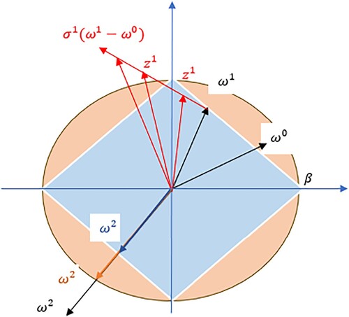
Figure 2. Training-validation accuracy plots of Algorithm 1 which is considered by the RLS$L_1$ ELM mode.

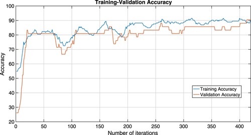
Figure 3. Training-validation loss plots of Algorithm 1 which is considered by the RLS$L_1$ ELM mode.

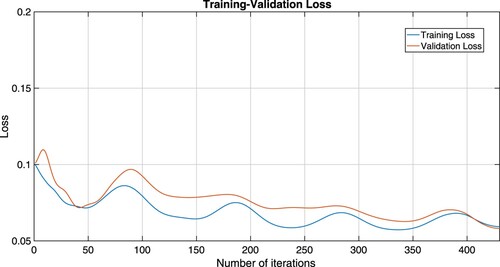
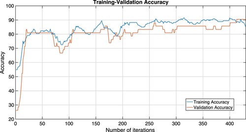
Figure 4. Training-validation accuracy plots of Algorithm 1 which is considered by the RLS$L_1$-C$L_2$ ELM mode.

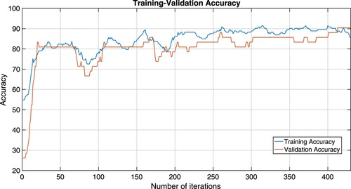
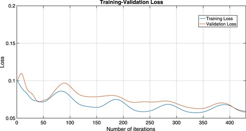
Figure 5. Training-validation loss plots of Algorithm 1 which is considered by the RLS$L_1$-C$L_2$ ELM mode.

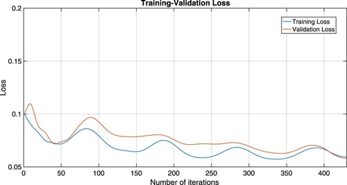
Figure 6. Training-validation accuracy plots of IMFB (3(3) $\begin{array}{rl}{y}^k& ={\omega }^k+{\sigma }^k({\omega }^k-{\omega }^{k-1}),\\ z^k& =y^k+{\alpha }^k({\omega }^k-y^k),\\ {\omega }^{k+1}& =J_{{\tau }^k}^{\mathbb{G}}(z^k-{\tau }^k\mathbb{F}{z}^k),k\ge 0,\end{array}$(3) ) which is considered by the RLS$L_1$ ELM mode.

Theorem 3.2

Let the sequence $\left\{{\omega }^k\right\}$ generated by Algorithm 1 satisfying the conditions $\left(C1\right)-\left(C3\right)$. Then, $\left\{{\omega }^k\right\}$ converges weakly to an element of Ψ.

Proof.

Let ${\omega }^{\ast }\in \mathrm{\Psi }$. Sine $P_{\mathbf{C}}$ and $J_{{\tau }^k}^{\mathbb{G}}(I-{\tau }^k\mathbb{F})$ are nonexpansive, we have (4) $\begin{array}{rl}\Vert {\omega }^{k+1}-{\omega }^{\ast }\Vert & =\Vert P_{\mathbf{C}}({\text{β}}^k{y}^k+(1-{\text{β}}^k\left)J_{{\tau }^k}^{\mathbb{G}}\right(I-{\tau }^k\mathbb{F}\left)y^k\right)-{\omega }^{\ast }\Vert \\ & \le \Vert {\text{β}}^k{y}^k+(1-{\text{β}}^k)J_{{\tau }^k}^{\mathbb{G}}(I-{\tau }^k\mathbb{F})y^k-{\omega }^{\ast }\Vert \\ & \le {\text{β}}^k\Vert y^k-{\omega }^{\ast }\Vert +(1-{\text{β}}^k)\Vert J_{{\tau }^k}^{\mathbb{G}}(I-{\tau }^k\mathbb{F})y^k-{\omega }^{\ast }\Vert \\ & \le \Vert y^k-{\omega }^{\ast }\Vert \\ & \le {\alpha }^k\Vert z^k-{\omega }^{\ast }\Vert +(1-{\alpha }^k)\Vert J_{{\tau }^k}^{\mathbb{G}}(I-{\tau }^k\mathbb{F})z^k-{\omega }^{\ast }\Vert \\ & \le \Vert z^k-{\omega }^{\ast }\Vert \\ & \le \Vert {\omega }^k-{\omega }^{\ast }\Vert +{\sigma }^k\Vert {\omega }^k-{\omega }^{k-1}\Vert .\end{array}$(4) By Lemma 2.8, we obtain that $\underset{n\to \mathrm{\infty }}{lim}\Vert {\omega }^k-{\omega }^{\ast }\Vert$ exists. Since $\Vert {\omega }^{k+1}-{\omega }^{\ast }\Vert \le \Vert y^k-{\omega }^{\ast }\Vert \le \Vert z^k-{\omega }^{\ast }\Vert \le \Vert {\omega }^k-{\omega }^{\ast }\Vert +{\sigma }^k\Vert {\omega }^k-{\omega }^{k-1}\Vert$, we also obtain (5) $\underset{n\to \mathrm{\infty }}{lim}\Vert {\omega }^k-{\omega }^{\ast }\Vert =\underset{n\to \mathrm{\infty }}{lim}\Vert y^k-{\omega }^{\ast }\Vert =\underset{n\to \mathrm{\infty }}{lim}\Vert z^k-{\omega }^{\ast }\Vert .$(5) This implies that $\left\{{\omega }^k\right\}$ is bounded and also $\left\{z^k\right\}$ and $\left\{\mathbb{F}{z}^k\right\}$ are also bounded. Since $\mathbb{F}$ is α-inverse-strongly monotone mapping by Lemma 2.5, then by (4(4) $\begin{array}{rl}\Vert {\omega }^{k+1}-{\omega }^{\ast }\Vert & =\Vert P_{\mathbf{C}}({\text{β}}^k{y}^k+(1-{\text{β}}^k\left)J_{{\tau }^k}^{\mathbb{G}}\right(I-{\tau }^k\mathbb{F}\left)y^k\right)-{\omega }^{\ast }\Vert \\ & \le \Vert {\text{β}}^k{y}^k+(1-{\text{β}}^k)J_{{\tau }^k}^{\mathbb{G}}(I-{\tau }^k\mathbb{F})y^k-{\omega }^{\ast }\Vert \\ & \le {\text{β}}^k\Vert y^k-{\omega }^{\ast }\Vert +(1-{\text{β}}^k)\Vert J_{{\tau }^k}^{\mathbb{G}}(I-{\tau }^k\mathbb{F})y^k-{\omega }^{\ast }\Vert \\ & \le \Vert y^k-{\omega }^{\ast }\Vert \\ & \le {\alpha }^k\Vert z^k-{\omega }^{\ast }\Vert +(1-{\alpha }^k)\Vert J_{{\tau }^k}^{\mathbb{G}}(I-{\tau }^k\mathbb{F})z^k-{\omega }^{\ast }\Vert \\ & \le \Vert z^k-{\omega }^{\ast }\Vert \\ & \le \Vert {\omega }^k-{\omega }^{\ast }\Vert +{\sigma }^k\Vert {\omega }^k-{\omega }^{k-1}\Vert .\end{array}$(4) ) and $J_{{\tau }^k}^{\mathbb{G}}$ is firmly nonexpansive mapping, we have $\begin{array}{rl}\Vert {\omega }^{k+1}-{\omega }^{\ast }{\Vert }^2& \le {\alpha }^k\Vert z^k-{\omega }^{\ast }{\Vert }^2+(1-{\alpha }^k)\Vert J_{{\tau }^k}^{\mathbb{G}}(I-{\tau }^k\mathbb{F})z^k-{\omega }^{\ast }{\Vert }^2\\ & \le {\alpha }^k\Vert z^k-{\omega }^{\ast }{\Vert }^2+(1-{\alpha }^k)(\Vert z^k-{\omega }^{\ast }-{\tau }^k(\mathbb{F}{z}^k-\mathbb{F}{\omega }^{\ast }){\Vert }^2\\ & -\Vert z^k-J_{{\tau }^k}^{\mathbb{G}}(I-{\tau }^k\mathbb{F})z^k-{\tau }^k(\mathbb{F}{z}^k-\mathbb{F}{\omega }^{\ast })\Vert )\\ & \le {\alpha }^k\Vert z^k-{\omega }^{\ast }{\Vert }^2+(1-{\alpha }^k)(\Vert z^k-{\omega }^{\ast }{\Vert }^2+({\tau }^k{)}^2\Vert \mathbb{F}{z}^k-\mathbb{F}{\omega }^{\ast }{\Vert }^2\\ & -2{\tau }^k〈z^k-{\omega }^{\ast },\mathbb{F}{z}^k-\mathbb{F}{\omega }^{\ast }〉\\ & -\Vert z^k-J_{{\tau }^k}^{\mathbb{G}}(I-{\tau }^k\mathbb{F})z^k-{\tau }^k(\mathbb{F}{z}^k-\mathbb{F}{\omega }^{\ast })\Vert )\\ & \le \Vert z^k-{\omega }^{\ast }{\Vert }^2-(1-{\alpha }^k)({\tau }^k(2\alpha -{\tau }^k)\Vert \mathbb{F}{z}^k-\mathbb{F}{\omega }^{\ast }{\Vert }^2\\ & +\Vert z^k-J_{{\tau }^k}^{\mathbb{G}}(I-{\tau }^k\mathbb{F})z^k-{\tau }^k(\mathbb{F}{z}^k-\mathbb{F}{\omega }^{\ast })\Vert ).\end{array}$ It follows from (5(5) $\underset{n\to \mathrm{\infty }}{lim}\Vert {\omega }^k-{\omega }^{\ast }\Vert =\underset{n\to \mathrm{\infty }}{lim}\Vert y^k-{\omega }^{\ast }\Vert =\underset{n\to \mathrm{\infty }}{lim}\Vert z^k-{\omega }^{\ast }\Vert .$(5) ) and $\underset{k\to \mathrm{\infty }}{lim sup}{\alpha }^k<1,0<\underset{k\to \mathrm{\infty }}{lim inf}{\tau }^k\le \underset{k\to \mathrm{\infty }}{lim sup}{\tau }^k<2\alpha$ and $\sum _{k=1}^{\mathrm{\infty }}{\sigma }^k\Vert {\omega }^k-{\omega }^{k-1}\Vert <\mathrm{\infty }$ that (6) $\underset{k\to \mathrm{\infty }}{lim}\Vert \mathbb{F}{z}^k-\mathbb{F}{\omega }^{\ast }\Vert =\underset{k\to \mathrm{\infty }}{lim}\Vert z^k-J_{{\tau }^k}^{\mathbb{G}}(I-{\tau }^k\mathbb{F})z^k\Vert =0.$(6) Sine $\underset{k\to \mathrm{\infty }}{lim inf}{\tau }^k>0$, there exists $\tau >0$ such that $0<\tau \le {\tau }^k$. By Lemma 2.6(ii), we obtain $\Vert z^k-J_{\tau }^{\mathbb{G}}(I-\tau \mathbb{F})z^k\Vert \le 2\Vert z^k-J_{{\tau }^k}^{\mathbb{G}}(I-{\tau }^k\mathbb{F})z^k\Vert .$ It follows from (6(6) $\underset{k\to \mathrm{\infty }}{lim}\Vert \mathbb{F}{z}^k-\mathbb{F}{\omega }^{\ast }\Vert =\underset{k\to \mathrm{\infty }}{lim}\Vert z^k-J_{{\tau }^k}^{\mathbb{G}}(I-{\tau }^k\mathbb{F})z^k\Vert =0.$(6) ) that (7) $\underset{k\to \mathrm{\infty }}{lim}\Vert z^k-J_{\tau }^{\mathbb{G}}(I-\tau \mathbb{F})z^k\Vert =0.$(7) We next let $\hat{\omega }$ be a weak sequential cluster point of $\left\{{\omega }^k\right\}$. Since $\mathbf{C}$ is closed convex set, $\hat{\omega }\in \mathbf{C}$. It follows from (5(5) $\underset{n\to \mathrm{\infty }}{lim}\Vert {\omega }^k-{\omega }^{\ast }\Vert =\underset{n\to \mathrm{\infty }}{lim}\Vert y^k-{\omega }^{\ast }\Vert =\underset{n\to \mathrm{\infty }}{lim}\Vert z^k-{\omega }^{\ast }\Vert .$(5) ) and (7(7) $\underset{k\to \mathrm{\infty }}{lim}\Vert z^k-J_{\tau }^{\mathbb{G}}(I-\tau \mathbb{F})z^k\Vert =0.$(7) ) that $\hat{\omega }\in \mathrm{\Psi }$ by Lemma 2.7. Since $\underset{k\to \mathrm{\infty }}{lim}\Vert {\omega }^k-\hat{\omega }\Vert$ exists, by Lemma 2.9, we obtain $\left\{{\omega }^k\right\}$ converges weakly to $\hat{\omega }$. Theorem 3.2 is completed.

4. Data classification problem

Parkinson's disease (PD) is a non-communicable disease that is a movement disorder characterized by the progressive degeneration of dopaminergic neurones in the midbrain. Its severity level is classified as stage 1, 2, 3, and severe condition. In the medical world, it is often difficult to identify the severity of Parkinson's disease and predict the progression of the disease. The disease often occurs in individuals older than 60. Parkinson's disease is a disease that, if not adequately treated, can lead to an inability to control walking, leading to accidents. and may cause disability risk. Therefore, if it is found that a family member has symptoms related to this disease, they should be taken to see a doctor immediately for treatment and to prevent harm to the patient. Therefore, using machine learning to help analyze the likelihood that a patient will likely develop a disease is very important. In this paper, we applied our proposed Algorithm 1 in an extreme learning machine (ELM) to find the optimal weights using the PD dataset from UCI Machine Learning Repository. This dataset is available online at the well-known UCI machine learning website [25] and was published in [26, 27]. The dataset consists of 23 attributes and 195 instances which were first created in a collaboration between Oxford University and the National Centre for Voice and Speech by Max Little. The overview of the data is shown in Table 1.

Table 1. The overview of PD dataset from UCI Machine Learning Repository.

Attribute Name	Description	Mean	Max	Min	SD	CV
MDVP:Fo (Hz)	Vocal fundamental (mean frequency)	154.2286	260.1050	88.33300	41.390065	0.268368
MDVP: Fhi(Hz)	Vocal fundamental (Max frequency)	197.1049	592.0300	102.1450	91.491548	0.464177
MDVP: Flo (Hz)	Vocal fundamental (Min frequency)	116.3246	239.1700	65.47600	43.521413	0.374138
MDVP:Jitter(%)	Basic frequency variations	0.006220	0.033160	0.001680	0.004848	0.779385
MDVP:Jitter(Abs)	Basic frequency variations	0.000044	0.000260	0.000007	0.000035	0.792145
MDVP:RAP	Basic frequency variations	0.003306	0.021440	0.000680	0.002968	0.897582
MDVHAL:PPQ	Basic frequency variations	0.003446	0.019580	0.000920	0.002759	0.800548
Jitter:DDP	Basic frequency variations	0.009920	0.064330	0.002040	0.008903	0.897519
MDVP:Berkilauan	Basic frequency variations	0.029709	0.119080	0.009540	0.018857	0.634718
MDVP:Berkilau(dB)	Wave variations	0.282251	1.302000	0.085000	0.194877	0.690439
Glitter:APQ3	Wave variations	0.015664	0.056470	0.004550	0.010153	0.648178
Glitter:APQ5	Wave variations	0.017878	0.079400	0.005700	0.012024	0.672532
MDVP:APQ	Wave variations	0.024081	0.137780	0.007190	0.016947	0.703725
Berkilauan:DDA	Wave variations	0.046993	0.169420	0.013640	0.030459	0.648168
NHR	The ratio of noise with regard to total components in voice	0.024847	0.314820	0.000650	0.040418	1.626688
HNR	The ratio of noise with regard to total components in voice	21.88597	33.04700	8.441000	4.425764	0.202219
RPDE	Nonlinear complexity measurements	0.498536	0.685151	0.256570	0.103942	0.208494
DFA	Fractal scaling exponent	0.718099	0.825288	0.574282	0.055336	0.077059
penyebaran1	Methods for calculating fundamental frequency variation	−5.684397	−2.434031	−7.964984	1.090208	−0.191790
penyebaran2	Methods for calculating fundamental frequency variation	0.226510	0.450493	0.006274	0.083406	0.368221
D2	Nonlinear complexity measurements	2.381826	3.671155	1.423287	0.382799	0.160717
PPE	Methods for calculating fundamental frequency variation	0.206552	0.527367	0.044539	0.090119	0.436304
Condition	Health status

Very recently, Elshewey et al. [17] presented using Bayesian optimization (BO) [28] or optimizing the hyperparameters of machine learning models: Support Vector Machine (SVM) [29], Random Forest (RF) [30], Logistic Regression (LR) [31], Naive Bayes (NB) [32], Ridge Classifier (RC) [33], and Decision Tree (DT) [34] to obtain better accuracy by using PD dataset with min–max normalization. Table 2 shows the different accuracy of the machine learning methods between using BO optimizing the hyperparameters and the default parameters compared with our algorithm in an extreme learning machine (ELM).

To understand ELM, which was first introduced by Huang et al. [35], we let $\mathbf{K}:=\left\{\right(x^k,b^k):x^k\in {\mathbb{R}}^n,b^k\in {\mathbb{R}}^m,k=1,2,\dots ,N\}$ be a training set of N distinct samples where $x^k$ is an input training data and $b^k$ is a training target. The output function of ELM for single-hidden layer feed forward neural networks (SLFNs) with L hidden nodes is $O^k=\sum _{i=1}^L{\omega }_{i}g(a_i{x}^k+b_i),$ where g is an activation function, $a_i$ and $b_i$ are parameters of weight and finally the bias at the i-th hidden node, respectively, and ${\omega }_i$ is the optimal output weight at the i-th hidden node. The hidden layer output matrix $\mathbf{A}$ is defined as follows: $\mathbf{A}=\left[\begin{array}{ccc}g(a_1{x}^1+b_1)& \dots & g(a_L{x}^1+b_L)\\ ⋮& \ddots & ⋮\\ g(a_1{x}^N+b_1)& \dots & g(a_L{x}^N+b_L)\end{array}\right]$ The main goal of ELM is to find optimal output weight $\omega =[{\omega }_1,\dots ,{\omega }_L{]}^T$ such that $\mathbf{A}\omega =\mathbf{B}$, where $\mathbf{B}=[b^1,\dots ,b^N{]}^T$ is the training target dataset. In some cases, finding the exact solution of a linear equation $\mathbf{A}\omega =\mathbf{B}$ may be difficult, therefore least square problem has been considered to approximate the solution. Also, for suitable prediction, overfitting of the model should be considered. In this paper, we avoid overfitting our model by using regularized least squares (RLS) and show the excellent fit of our model by considering accuracy and loss porting. The six regularized least squares problem models can be solved by our proposed algorithm by setting as follows: for a regularization parameter $\lambda >0$ and constrained constant $\text{β}>0$,

1. setting $\mathbb{F}\left(\omega \right)\equiv \mathrm{\nabla }(\frac{1}{2}\Vert \mathbf{A}\omega -\mathbf{B}{\Vert }_2^2)$, $\mathbb{G}\left(\omega \right)\equiv \mathrm{\partial }(\lambda \Vert \omega {\Vert }_1)$, $\mathbf{C}=\mathbf{H}$ in regularized least squares by $L_1$ (RLS$L_1$) (8) $\underset{\omega \in {\mathbb{R}}^L}{min}\{\frac{1}{2}\Vert \mathbf{A}\omega -\mathbf{B}{\Vert }_2^2+\lambda \Vert \omega {\Vert }_1\};$(8)

2. setting $\mathbb{F}\left(\omega \right)\equiv \mathrm{\nabla }(\frac{1}{2}\Vert \mathbf{A}\omega -\mathbf{B}{\Vert }_2^2)$, $\mathbb{G}\left(\omega \right)\equiv \mathrm{\partial }(\lambda \Vert \omega {\Vert }_2^2)$, $\mathbf{C}=\mathbf{H}$ in regularized least squares by $L_2$ (RLS$L_2$) (9) $\underset{\omega \in {\mathbb{R}}^L}{min}\{\frac{1}{2}\Vert \mathbf{A}\omega -\mathbf{B}{\Vert }_2^2+\lambda \Vert \omega {\Vert }_2^2\};$(9)

3. setting $\mathbb{F}\left(\omega \right)\equiv \mathrm{\nabla }(\frac{1}{2}\Vert \mathbf{A}\omega -\mathbf{B}{\Vert }_2^2)$, $\mathbb{G}\left(\omega \right)\equiv \mathrm{\partial }(\lambda \Vert \omega {\Vert }_1)$, $\mathbf{C}=\{\omega :\Vert \omega {\Vert }_1\le \text{β}\}$ in regularized least squares by $L_1$ on constrained set $\mathbf{C}$ (RLS$L_1$-C$L_1$) (10) $\underset{\omega \in \mathbf{C}}{min}\{\frac{1}{2}\Vert \mathbf{A}\omega -\mathbf{B}{\Vert }_2^2+\lambda \Vert \omega {\Vert }_1\};$(10)

4. setting $\mathbb{F}\left(\omega \right)\equiv \mathrm{\nabla }(\frac{1}{2}\Vert \mathbf{A}\omega -\mathbf{B}{\Vert }_2^2)$ , $\mathbb{G}\left(\omega \right)\equiv \mathrm{\partial }(\lambda \Vert \omega {\Vert }_1)$, $\mathbf{C}=\{\omega :\Vert \omega {\Vert }_2^2\le \text{β}\}$ in regularized least squares by $L_1$ on constrained set $\mathbf{C}$ (RLS$L_1$-C$L_2$) (11) $\underset{\omega \in \mathbf{C}}{min}\{\frac{1}{2}\Vert \mathbf{A}\omega -\mathbf{B}{\Vert }_2^2+\lambda \Vert \omega {\Vert }_1\};$(11)

5. setting $\mathbb{F}\left(\omega \right)\equiv \mathrm{\nabla }(\frac{1}{2}\Vert \mathbf{A}\omega -\mathbf{B}{\Vert }_2^2)$ , $\mathbb{G}\left(\omega \right)\equiv \mathrm{\partial }(\lambda \Vert \omega {\Vert }_2^2)$, $\mathbf{C}=\{\omega :\Vert \omega {\Vert }_1\le \text{β}\}$ in regularized least squares by $L_2$ on constrained set $\mathbf{C}$ (RLS$L_2$-C$L_1$) (12) $\underset{\omega \in \mathbf{C}}{min}\{\frac{1}{2}\Vert \mathbf{A}\omega -\mathbf{B}{\Vert }_2^2+\lambda \Vert \omega {\Vert }_2^2\};$(12)

6. setting $\mathbb{F}\left(\omega \right)\equiv \mathrm{\nabla }(\frac{1}{2}\Vert \mathbf{A}\omega -\mathbf{B}{\Vert }_2^2)$ , $\mathbb{G}\left(\omega \right)\equiv \mathrm{\partial }(\lambda \Vert \omega {\Vert }_2^2)$, $\mathbf{C}=\{\omega :\Vert \omega {\Vert }_2^2\le \text{β}\}$ in regularized least squares by $L_2$ on constrained set $\mathbf{C}$ (RLS$L_2$-C$L_2$) (13) $\underset{\omega \in \mathbf{C}}{min}\{\frac{1}{2}\Vert \mathbf{A}\omega -\mathbf{B}{\Vert }_2^2+\lambda \Vert \omega {\Vert }_2^2\}.$(13)

Table 2. The accuracy comparison between Elshewey et al. [17] methods and ours.

	Default parameters	BO for optimizing the hyperparameters
SVM	89.6	92.3
RF	87.2	89.7
LR	85.3	87.2
NB	82.1	84.6
RC	80.9	83.3
DT	85.7	88.5
Our ELM	92.86

Remark 4.1

The novelty of Algorithm 1 is applied to solve regularization problem models on constrained sets in many directions (10(10) $\underset{\omega \in \mathbf{C}}{min}\{\frac{1}{2}\Vert \mathbf{A}\omega -\mathbf{B}{\Vert }_2^2+\lambda \Vert \omega {\Vert }_1\};$(10) )–(13(13) $\underset{\omega \in \mathbf{C}}{min}\{\frac{1}{2}\Vert \mathbf{A}\omega -\mathbf{B}{\Vert }_2^2+\lambda \Vert \omega {\Vert }_2^2\}.$(13) ) which is different from algorithms in the literature and achieves good results.

The binary cross entropy loss function calculates the loss of an example by computing the following average: $\mathrm{Loss}=-\frac{1}{\mathrm{output}\mathrm{size}}\sum _{k=1}^{\mathrm{output}\mathrm{size}}{O}^k\log {\hat{O}}^k+(1-O^k)\log (1-{\hat{O}}^k)$ where ${\hat{O}}^k$ is the k-th scalar value in the model output, $O^k$ is the corresponding target value, and the output size is the number of scalar values in the model output.

In this work, we present four measures: Accuracy, Recall, Precision, and F1-score for the performance reports. The formulations of three measures are defined as follows: $\begin{array}{rl}\mathrm{Precision}\left(\mathrm{Pre}\right)& =\frac{\mathrm{TP}}{\mathrm{TP}+\mathrm{FP}}\times 100\mathrm{\%}.\\ \mathrm{Recall}\left(\mathrm{Rec}\right)& =\frac{\mathrm{TP}}{\mathrm{TP}+\mathrm{FN}}\times 100\mathrm{\%}.\\ \mathrm{Accuracy}\left(\mathrm{Acc}\right)& =\frac{\mathrm{TP}+\mathrm{TN}}{\mathrm{TP}+\mathrm{FP}+\mathrm{TN}+\mathrm{FN}}\times 100\mathrm{\%},\\ F1-\mathrm{score}& =\frac{2\times (\mathrm{Precision}\times \mathrm{Recall})}{\mathrm{Precision}+\mathrm{Recall}},\end{array}$ where $\mathrm{TN}$:=True Negative, $\mathrm{FP}$:= False Positive, $\mathrm{FN}$:=False Negative, and $\mathrm{TP}$:=True Positive.

For comparison experiments, optimization models (8(8) $\underset{\omega \in {\mathbb{R}}^L}{min}\{\frac{1}{2}\Vert \mathbf{A}\omega -\mathbf{B}{\Vert }_2^2+\lambda \Vert \omega {\Vert }_1\};$(8) ) and (9(9) $\underset{\omega \in {\mathbb{R}}^L}{min}\{\frac{1}{2}\Vert \mathbf{A}\omega -\mathbf{B}{\Vert }_2^2+\lambda \Vert \omega {\Vert }_2^2\};$(9) ) are considered for IFB (2(2) $\begin{array}{rl}{y}^k& ={\omega }^k+{\sigma }^k({\omega }^k-{\omega }^{k-1}),\\ {\omega }^{k+1}& =J_{{\tau }^k}^{\mathbb{G}}(y^k-{\tau }^k\mathbb{F}{\omega }^k),k\ge 0,\end{array}$(2) ) and IMFB (3(3) $\begin{array}{rl}{y}^k& ={\omega }^k+{\sigma }^k({\omega }^k-{\omega }^{k-1}),\\ z^k& =y^k+{\alpha }^k({\omega }^k-y^k),\\ {\omega }^{k+1}& =J_{{\tau }^k}^{\mathbb{G}}(z^k-{\tau }^k\mathbb{F}{z}^k),k\ge 0,\end{array}$(3) ) algorithms. The necessary parameters which are used in our Algorithm 1, IFB (2(2) $\begin{array}{rl}{y}^k& ={\omega }^k+{\sigma }^k({\omega }^k-{\omega }^{k-1}),\\ {\omega }^{k+1}& =J_{{\tau }^k}^{\mathbb{G}}(y^k-{\tau }^k\mathbb{F}{\omega }^k),k\ge 0,\end{array}$(2) ) and IMFB (3(3) $\begin{array}{rl}{y}^k& ={\omega }^k+{\sigma }^k({\omega }^k-{\omega }^{k-1}),\\ z^k& =y^k+{\alpha }^k({\omega }^k-y^k),\\ {\omega }^{k+1}& =J_{{\tau }^k}^{\mathbb{G}}(z^k-{\tau }^k\mathbb{F}{z}^k),k\ge 0,\end{array}$(3) ) algorithms can be seen in Table 3 where ${\sigma }^k=\{\begin{array}{ll}\frac{\sigma }{k^2\Vert {\omega }^k-{\omega }^{k-1}}\Vert & \mathrm{if}k>K\mathrm{and}{\omega }^k\ne {\omega }^{k-1},\\ \sigma & \mathrm{otherwise},\end{array}$ where K is a number of iterations that we want to stop.

Table 3. The necessary parameters for our Algorithm 1, IFB (2(2) $\begin{array}{rl}{y}^k& ={\omega }^k+{\sigma }^k({\omega }^k-{\omega }^{k-1}),\\ {\omega }^{k+1}& =J_{{\tau }^k}^{\mathbb{G}}(y^k-{\tau }^k\mathbb{F}{\omega }^k),k\ge 0,\end{array}$(2) ) and IMFB (3(3) $\begin{array}{rl}{y}^k& ={\omega }^k+{\sigma }^k({\omega }^k-{\omega }^{k-1}),\\ z^k& =y^k+{\alpha }^k({\omega }^k-y^k),\\ {\omega }^{k+1}& =J_{{\tau }^k}^{\mathbb{G}}(z^k-{\tau }^k\mathbb{F}{z}^k),k\ge 0,\end{array}$(3) ).

	Optimization model	σ	${\alpha }^k$	${\text{β}}^k$	${\tau }^k$	λ	β
Algorithm 1	RLS$L_1$	0.9999	$\frac{n}{{10}^{6}n+1}$	$\frac{n}{{10}^{6}n+1}$	$\frac{0.999}{\Vert \mathbf{A}{\Vert }^2}$	0.1	–
	RLS$L_2$	0.9999	$\frac{n}{{10}^{6}n+1}$	$\frac{n}{{10}^{6}n+1}$	$\frac{0.999}{\Vert \mathbf{A}{\Vert }^2}$	1000	–
	RLS$L_1$-C$L_1$	0.9999	$\frac{n}{{10}^{6}n+1}$	$\frac{n}{{10}^{6}n+1}$	$\frac{0.999}{\Vert \mathbf{A}{\Vert }^2}$	0.1	61
	RLS$L_1$-C$L_2$	0.9999	$\frac{n}{{10}^{6}n+1}$	$\frac{n}{{10}^{6}n+1}$	$\frac{0.999}{\Vert \mathbf{A}{\Vert }^2}$	0.1	20
	RLS$L_2$-C$L_1$	0.9999	$\frac{n}{{10}^{6}n+1}$	$\frac{n}{{10}^{6}n+1}$	$\frac{0.999}{\Vert \mathbf{A}{\Vert }^2}$	1000	60
	RLS$L_2$-C$L_2$	0.9999	$\frac{n}{{10}^{6}n+1}$	$\frac{n}{{10}^{6}n+1}$	$\frac{0.999}{\Vert \mathbf{A}{\Vert }^2}$	1000	40
IFB (2(2) $\begin{array}{rl}{y}^k& ={\omega }^k+{\sigma }^k({\omega }^k-{\omega }^{k-1}),\\ {\omega }^{k+1}& =J_{{\tau }^k}^{\mathbb{G}}(y^k-{\tau }^k\mathbb{F}{\omega }^k),k\ge 0,\end{array}$(2) )	RLS$L_1$	0.9999	–	–	$\frac{0.2}{\Vert \mathbf{A}{\Vert }^2}$	0.1	–
	RLS$L_2$	0.9999	–	–	$\frac{0.2}{\Vert \mathbf{A}{\Vert }^2}$	0.1	–
IMFB (3(3) $\begin{array}{rl}{y}^k& ={\omega }^k+{\sigma }^k({\omega }^k-{\omega }^{k-1}),\\ z^k& =y^k+{\alpha }^k({\omega }^k-y^k),\\ {\omega }^{k+1}& =J_{{\tau }^k}^{\mathbb{G}}(z^k-{\tau }^k\mathbb{F}{z}^k),k\ge 0,\end{array}$(3) )	RLS$L_1$	0.9999	$\frac{n}{{10}^{6}n+1}$	–	$\frac{0.999}{\Vert \mathbf{A}{\Vert }^2}$	0.1	–
	RLS$L_2$	0.9999	$\frac{n}{{10}^{6}n+1}$	–	$\frac{0.999}{\Vert \mathbf{A}{\Vert }^2}$	1000	–

This experiment, we use sigmoid as an activation function and 130 hidden nodes. The results of all algorithms our Algorithm 1, IFB (2(2) $\begin{array}{rl}{y}^k& ={\omega }^k+{\sigma }^k({\omega }^k-{\omega }^{k-1}),\\ {\omega }^{k+1}& =J_{{\tau }^k}^{\mathbb{G}}(y^k-{\tau }^k\mathbb{F}{\omega }^k),k\ge 0,\end{array}$(2) ) and IMFB (3(3) $\begin{array}{rl}{y}^k& ={\omega }^k+{\sigma }^k({\omega }^k-{\omega }^{k-1}),\\ z^k& =y^k+{\alpha }^k({\omega }^k-y^k),\\ {\omega }^{k+1}& =J_{{\tau }^k}^{\mathbb{G}}(z^k-{\tau }^k\mathbb{F}{z}^k),k\ge 0,\end{array}$(3) ) are shown in Table 4.

From Table 4, we see that our Algorithm 1 when it's considered by the RLS$L_1$ and RLS$L_1$-C$L_2$ ELM model gives the highest accuracy precision, recall, and F1-score efficiency, respectively. To show that our Algorithm is efficient without model over-fitting, we consider the following training and validation loss with the accuracy plots.

From Figures 2–7, we see that training-validation loss, and accuracy plots are almost the same throughout, even though they oscillate, indicating that our models are well fitting. This means that our machine learning model adapts well to data similar to the data on which it was trained.

Figure 7. Training-validation loss plots of IMFB (3(3) $\begin{array}{rl}{y}^k& ={\omega }^k+{\sigma }^k({\omega }^k-{\omega }^{k-1}),\\ z^k& =y^k+{\alpha }^k({\omega }^k-y^k),\\ {\omega }^{k+1}& =J_{{\tau }^k}^{\mathbb{G}}(z^k-{\tau }^k\mathbb{F}{z}^k),k\ge 0,\end{array}$(3) ) which is considered by the RLS$L_1$ ELM mode.

Table 4. The performance by 4 evaluation matrices of our Algorithm 1, IFB (2(2) $\begin{array}{rl}{y}^k& ={\omega }^k+{\sigma }^k({\omega }^k-{\omega }^{k-1}),\\ {\omega }^{k+1}& =J_{{\tau }^k}^{\mathbb{G}}(y^k-{\tau }^k\mathbb{F}{\omega }^k),k\ge 0,\end{array}$(2) ) and IMFB (3(3) $\begin{array}{rl}{y}^k& ={\omega }^k+{\sigma }^k({\omega }^k-{\omega }^{k-1}),\\ z^k& =y^k+{\alpha }^k({\omega }^k-y^k),\\ {\omega }^{k+1}& =J_{{\tau }^k}^{\mathbb{G}}(z^k-{\tau }^k\mathbb{F}{z}^k),k\ge 0,\end{array}$(3) ).

	Optimization model	Number of Iterations	Training Time	Accuracy	Precision	Recall	F1-score
Algorithm 1	RLS$L_1$	433	0.0680	92.86	62.50	100	76.92
	RLS$L_2$	314	0.0631	88.10	37.50	100	54.55
	RLS$L_1$-C$L_1$	449	0.0856	92.86	62.50	100	76.92
	RLS$L_1$-C$L_2$	433	0.0849	92.86	62.50	100	76.92
	RLS$L_2$-C$L_1$	431	0.0818	90.48	62.50	83.88	71.43
	RLS$L_2$-C$L_2$	314	0.0640	88.10	37.50	100	54.55
IFB (2(2) $\begin{array}{rl}{y}^k& ={\omega }^k+{\sigma }^k({\omega }^k-{\omega }^{k-1}),\\ {\omega }^{k+1}& =J_{{\tau }^k}^{\mathbb{G}}(y^k-{\tau }^k\mathbb{F}{\omega }^k),k\ge 0,\end{array}$(2) )	RLS$L_1$	55	0.0170	83.33	12.50	100	22.22
	RLS$L_2$	185	0.0325	80.05	100	19.05	32.00
IMFB (3(3) $\begin{array}{rl}{y}^k& ={\omega }^k+{\sigma }^k({\omega }^k-{\omega }^{k-1}),\\ z^k& =y^k+{\alpha }^k({\omega }^k-y^k),\\ {\omega }^{k+1}& =J_{{\tau }^k}^{\mathbb{G}}(z^k-{\tau }^k\mathbb{F}{z}^k),k\ge 0,\end{array}$(3) )	RLS$L_1$	433	0.0748	92.86	62.50	100	76.92
	RLS$L_2$	314	0.0659	88.10	37.50	100	54.55

5. Conclusion

In this paper, we study extreme learning machine and introduce a new modified projective forward-backward splitting algorithm to solve variational inclusion problems. We also prove weak convergence theorem under mind condition on the control stepsize. Parkinson's disease dataset from UCI machine learning repository was used for data training applying the proposed algorithm. The comparison with other machine learning models and existing algorithms show that our algorithm provides the highest performance value of 92.86% accuracy, 62.50% precision, 100% recall, and 76.92% F1-score considering on regularized least squares by $L_1$ (RLS$L_1$) and regularized least squares by $L_1$ on constrained set $\mathbf{C}$ (RLS$L_1$-C$L_2$). Moreover, considering training and validation loss, and the accuracy plots show that our algorithm has good fit model. Our future research is to develop a more relaxed condition of the inertial extrapolation parameter ${\sigma }^k$. We also develop forward-backward splitting algorithms for multi-layer ELM (deep learning), which would be interesting to apply in machine learning.

Author's contributions

Writing – Original Draft and Software, W.C.; Review and Editing, S.D.. All authors have contributed to the development of each section of the paper and finally read and approved it for publication.

Disclosure statement

The authors have no competing interests to declare that are relevant to the content of this article.

Data availability statement

Parkinson's disease dataset is available on the UCI website (https://archive.ics.uci.edu/ml/datasets/parkinsons).

Additional information

Funding

This work is supported by National Research Council of Thailand and University of Phayao (N42A650334), and Thailand Science Research and Innovation, University of Phayao (FF67).

References

- Bauschke HH, Borwein JM. On projection algorithms for solving convex feasibility problems. SIAM Rev. 1996;38:367–426. doi: 10.1137/S0036144593251710
- Bauschke HH, Combettes PL. Convex analysis and monotone operator theory in Hilbert spaces. Berlin: Springer; 2011.
- Chen M, Li Y, Luo X, et al. A novel human activity recognition scheme for smart health using multilayer extreme learning machine. IEEE Internet Things J. 2019;6:1410–1418. doi: 10.1109/JIoT.6488907
- Polyak B. Some methods of speeding up the convergence of iteration methods. USSR Comput Math Math Phys. 1964;4(5):1–17. doi: 10.1016/0041-5553(64)90137-5
- Bot RI, Csetnek ER. An inertial forward-backward-forward primal-dual splitting algorithm for solving monotone inclusion problems. Numer Algorithms. 2016;71(3):519–540. doi: 10.1007/s11075-015-0007-5
- Hanjing A, Bussaban L, Suantai S. The modified viscosity approximation method with inertial technique and Forward–Backward algorithm for convex optimization model. Mathematics. 2022;10(7):1036. doi: 10.3390/math10071036
- Inthakon W, Suantai S, Sarnmeta P, et al. A new machine learning algorithm based on optimization method for regression and classification problems. Mathematics. 2020;8(6):1007. doi: 10.3390/math8061007
- Peeyada P, Dutta H, Shiangjen K, et al. A modified forward-backward splitting methods for the sum of two monotone operators with applications to breast cancer prediction. Math Methods Appl Sci. 2023;46(1):1251–1265. doi: 10.1002/mma.v46.1
- Tan B, Cho SY. Strong convergence of inertial forward–backward methods for solving monotone inclusions. Appl Anal. 2022;101(15):5386–5414. doi: 10.1080/00036811.2021.1892080
- Moudafi A, Oliny M. Convergence of a splitting inertial proximal method for monotone operators. J Comput Appl Math. 2003;155:447–454. doi: 10.1016/S0377-0427(02)00906-8
- Peeyada P, Suparatulatorn R, Cholamjiak W. An inertial Mann forward-backward splitting algorithm of variational inclusion problems and its applications. Chaos Solit Fractals. 2022;158:112048. doi: 10.1016/j.chaos.2022.112048
- Al-Dhaifallah M, Nisar KS, Agarwal P, et al. Modeling and identification of heat exchanger process using least squares support vector machines. Therm Sci. 2017;21(6 Part B):2859–2869. doi: 10.2298/TSCI151026204A
- Baleanu D, Hasanabadi M, Vaziri AM, et al. A new intervention strategy for an HIV/AIDS transmission by a general fractional modeling and an optimal control approach. Chaos Solit Fractals. 2023;167:113078. doi: 10.1016/j.chaos.2022.113078
- Baleanu D, Arshad S, Jajarmi A, et al. Dynamical behaviours and stability analysis of a generalized fractional model with a real case study. J Adv Res. 2023;48:157–173. doi: 10.1016/j.jare.2022.08.010
- Boonsatit N, Rajchakit G, Sriraman R, et al. Finite-fixed-time synchronization of delayed Clifford-valued recurrent neural networks. Adv Differ Equ. 2021;2021(1):1–25. doi: 10.1186/s13662-021-03438-1
- Rajchakit G, Agarwal P, Ramalingam S. Stability analysis of neural networks. Singapore: Springer; 2021.
- Elshewey AM, Shams MY, El-Rashidy N, et al. Bayesian optimization with support vector machine model for Parkinson disease classification. Sensors. 2023;23(4):2085. doi: 10.3390/s23042085
- Chen HL, Wang G, Ma C, et al. An efficient hybrid kernel extreme learning machine approach for early diagnosis of Parkinson's disease. Neurocomputing. 2016;184:131–144. doi: 10.1016/j.neucom.2015.07.138
- Bauschke HH, Combettes PL. Convex analysis and monotone operator theory in Hilbert spaces. New York: Springer; 2011. (CMS Books in Mathematics).
- Brézis H. Opérateurs maximaux monotones et semi-groupes de contractions dans les espaces de Hilbert. Amsterdam, Netherlands: North-Holland; 1973. (Math. Studies 5).
- Zhang J, Li Y, Xiao W, et al. Non-iterative and fast deep learning: multilayer extreme learning machines. J Franklin Inst B. 2020;357(13):8925–8955. doi: 10.1016/j.jfranklin.2020.04.033
- López G, Martn-Mrquez V, Wang F, et al. Forward-backward splitting methods for accretive operators in Banach spaces. Abstr Appl Anal. 2012;2012:109236.
- Goebel K, Kirk WA. Topics in metric fixed point theory. Cambridge: Cambridge University Press; 1990.
- Auslender A, Teboulle M, Ben-Tiba S. A logarithmic-quadratic proximal method for variational inequalities. Boston, MA: Springer; 1999.
- Dua D, Graff C. UCI machine learning repository. Irvine, CA: University of California, School of Information and Computer Science; 2019. Available at http://archive.ics.uci.edu/ml.
- Little M, Mcsharry P, Roberts S, et al. Exploiting nonlinear recurrence and fractal scaling properties for voice disorder detection. Nat Preced. 2007;2007:1–1.
- Little M, McSharry P, Hunter E, et al. Suitability of dysphonia measurements for telemonitoring of Parkinson's disease. Nat Preced. 2008;2008:1–1.
- Cho H, Kim Y, Lee E, et al. Basic enhancement strategies when using Bayesian optimization for hyperparameter tuning of deep neural networks. IEEE Access. 2020;8:52588–52608. doi: 10.1109/Access.6287639
- Jakkula V. Tutorial on support vector machine (SVM). Sch EECS Wash State Univ. 2006;37:3.
- Cutler A, Cutler DR, Stevens JR. Random forests. In: Zhang C, Ma Y, editors. Ensemble machine learning. Berlin, Germany: Springer; 2012. p. 157–175.
- Nick TG, Campbell KM. Logistic regression. Top Biostat. 2007;404:273–301. doi: 10.1007/978-1-59745-530-5
- Zhang H. The optimality of naive Bayes. Aa. 2004;1(2):3.
- Xingyu MA, Bolei MA, Qi F. Logistic regression and ridge classifier; 2022.
- Kotsiantis SB. Decision trees: a recent overview. Artif Intell Rev. 2013;39:261–283. doi: 10.1007/s10462-011-9272-4
- Huang GB, Zhu QY, Siew CK. Extreme learning machine: a new learning scheme of feedforward neural networks. In 2004 IEEE international joint conference on neural networks, IEEE Cat. 2004;2(04CH37541):985–990.