Numerical method for a Cauchy problem for multi-dimensional Helmholtz equation

Abstract

The main focus of this research is to address the Cauchy problem of the multi-dimensional Helmholtz equation with mixed boundary conditions. This problem is known to be ill-posed according to Hadamard's definition. To tackle this issue, we propose the mollification regularization method based on exponential decay. Using prior rule and posterior rule to create a regular approximation solution and convergence of the solution is also provided. Furthermore, the proposed method is shown to be robust against data disruption noise, making it a reliable approach for solving the Cauchy problem of the multi-dimensional Helmholtz equation with mixed boundary conditions.

Keywords:

• Multi-dimensional Helmholtz equation
• mollification method
• exponential decay kernel
• Cauchy problem
• error estimate

Mathematics Subject Classifications:

• 35-00
• 35C06
• 35C05
• 65M32
• 35R30

1. Introduction

The inverse problem of the Helmholtz equation has found numerous applications in various fields such as geomorphology, quality exploration, remote sensing research, and optical signal processing. These applications span across technologies like microwave, radar, sonar, and laser. Given its significance, finding a numerical solution for the Helmholtz equation has been a prominent research area for almost 50 years. The specific form of the solution depends on the boundary conditions, which can be Dirichlet, Neumann, or a combination of both. However, according to Hadamard, the problem is considered extremely ill-posed. This means that even small changes in the input data can lead to significant changes in the solution. Therefore, it is crucial to develop an algorithm that is precise, stable, reliable, and efficient for solving the Cauchy problem associated with the Helmholtz equation.

The uniqueness and stability of the inverse Helmholtz problem have been investigated by several researchers [1–6]. In order to solve this problem numerically, various methods have been proposed. These include the Fourier transform [7–9], the continuation approach [10], the linear sampling technique [11,12], the Landweber regular method (BEM) [13], the Tikhonov regular method [14], and the mollification regularization method [15]. These numerical methods for addressing the inverse problem of the Helmholtz equation and applied in various research studies.

While the multi-dimensional Helmholtz equation is used in various applications, there has been relatively limited research specifically focussed on the multi-dimensional Helmholtz equation. Many existing numerical methods for solving the Helmholtz equation are primarily developed for one-dimensional or two-dimensional problems and may not be easily generalized to the multi-dimensional case. The multi-dimensional Helmholtz equation presents additional challenges due to the increased complexity of the problem. The higher dimensionality introduces more variables and parameters, making it more difficult to find efficient and accurate numerical solutions. As a result, there is a need for further research and development of numerical methods that are specifically to address the multi-dimensional Helmholtz equation. It can be seen from the references that the exponential decay kernel has great advantages in dealing with the inverse problems of fractional partial differential equations. Unfortunately, it has not been found that an exponential decay kernel is used to solve the Cauchy problem of the Helmholtz equation. Based on the above consideration, this paper presents a mollification regularization method of exponential decay kernel to solve the Cauchy problem of the multi-dimensional Helmholtz equation. The validity and stability of the proposed method are verified theoretically and numerically.

The idea behind the mollification approach is that if the data is provided inaccurately, we want to use a mollification operator that will turn the incorrect data into issue types that are well-posed, like [16–20]. In this paper, we solve the Cauchy problem using the mollification method based on an exponential decay kernel and show that our solution is stable and effective.

The structure of this essay is as follows: The ill-posed of Problem (1(2.1) $\{\begin{array}{l}\mathrm{\Delta }w(x,\mathbf{y})+k^{2}w(x,\mathbf{y})=0,0<x<1,\mathbf{y}\in R^n,\\ w(0,\mathbf{y})=\phi (\mathbf{y}),\mathbf{y}\in R^n,\\ w_x(0,\mathbf{y})=\psi (\mathbf{y}),\mathbf{y}\in R^n,\end{array}$(2.1) ) is demonstrated in Section 2. We explain the exponential decay kernel and some of its characteristics in Section 3. Some error estimate findings are given in 0<x<1 and at boundary x = 1 in Section 4. In Section 5, numerical experiments are used to show the method's effectiveness.

2. Model problem and its ill-posedness

Consider the following (2.1) $\{\begin{array}{l}\mathrm{\Delta }w(x,\mathbf{y})+k^{2}w(x,\mathbf{y})=0,0<x<1,\mathbf{y}\in R^n,\\ w(0,\mathbf{y})=\phi (\mathbf{y}),\mathbf{y}\in R^n,\\ w_x(0,\mathbf{y})=\psi (\mathbf{y}),\mathbf{y}\in R^n,\end{array}$(2.1) here multi-dimensional Laplace operator is $\mathrm{\Delta }=\frac{{\mathrm{\partial }}^2}{\mathrm{\partial }{y}_1^2}+\frac{{\mathrm{\partial }}^2}{\mathrm{\partial }{y}_2^2}+\cdot \cdot \cdot +\frac{{\mathrm{\partial }}^2}{\mathrm{\partial }{y}_n^2}$ and wave number is constant k>0. The data $\phi ,\psi$ must be used to calculate the solution $w(x,\mathbf{y})$, however they can only be measured. Since there exist measurement mistakes which recorded as: (${\phi }^{\delta }(y),{\psi }^{\delta }(y)$) and satisfy (2.2) $\Vert {\phi }^{\delta }-\phi {\Vert }_{H^p}+\Vert {\psi }^{\delta }-\psi {\Vert }_{H^p}\le \delta .$(2.2) The level of error is represented by the constant $\delta >0$ here. $\Vert f(\cdot ){\Vert }_{H^p}:=({\int }_{R^n}(1+{\eta }^2{)}^p|\hat{f}(\eta ){|}^2\mathrm{d}\eta {)}^{\frac{1}{2}}.$The Fourier transform of the function $f(\mathbf{y})$ is $\hat{f}(\eta )=\frac{1}{(2\pi {)}^{n/2}}{\int }_{R^n}f(\mathbf{y}){\mathrm{e}}^{-\mathrm{i\eta }.\mathbf{y}}\mathrm{d}\mathbf{y},\mathbf{y}\in R^n.$$f(\mathbf{y})$'s inverse Fourier transform is $f(\mathbf{y})=\frac{1}{(2\pi {)}^{n/2}}{\int }_{R^n}\hat{f}(\eta ){\mathrm{e}}^{\mathrm{i\eta }.\mathbf{y}}\mathrm{d}\xi .$If p = 0, then $H^0(R^n)=L^2(R^n)$.

According to the superposition principle of solutions, the solution of problem (1(2.1) $\{\begin{array}{l}\mathrm{\Delta }w(x,\mathbf{y})+k^{2}w(x,\mathbf{y})=0,0<x<1,\mathbf{y}\in R^n,\\ w(0,\mathbf{y})=\phi (\mathbf{y}),\mathbf{y}\in R^n,\\ w_x(0,\mathbf{y})=\psi (\mathbf{y}),\mathbf{y}\in R^n,\end{array}$(2.1) ) is the sum of the following two problems (2.3) $\{\begin{array}{l}\mathrm{\Delta }{w}_1(x,\mathbf{y})+k^2{w}_1(x,\mathbf{y})=0,0<x<1,\mathbf{y}\in R^n,\\ w_1(0,\mathbf{y})=\phi (\mathbf{y}),\mathbf{y}\in R^n,\\ (w_1{)}_x(0,\mathbf{y})=0,\mathbf{y}\in R^n\end{array}$(2.3) and (2.4) $\{\begin{array}{l}\mathrm{\Delta }{w}_2(x,\mathbf{y})+k^2{w}_2(x,\mathbf{y})=0,0<x<1,\mathbf{y}\in R^n,\\ w_2(0,\mathbf{y})=0,\mathbf{y}\in R^n,\\ (w_2{)}_x(0,\mathbf{y})=\psi (\mathbf{y}),\mathbf{y}\in R^n\end{array}$(2.4) Using the Fourier transform for the variable $\mathbf{y}\in R^n$, we obtain (2.5) $\{\begin{array}{l}{\widehat{(w_1)}}_{\mathrm{xx}}+({\eta }^2+k^2)\widehat{w_1}=0,0<x<1,\eta \in R^n,\\ \widehat{w_1}(0,\eta )=\hat{\phi }(\eta ),\eta \in R^n,\\ (\widehat{w_1}{)}_x(0,\eta )=0,\eta \in R^n\end{array}$(2.5) and (2.6) $\{\begin{array}{l}{\widehat{(w_2)}}_{\mathrm{xx}}+({\eta }^2+k^2)\widehat{w_2}=0,0<x<1,\eta \in R^n,\\ \widehat{w_2}(0,\eta )=0,\eta \in R^n,\\ (\widehat{w_2}{)}_x(0,\eta )=\hat{\psi }(\eta ),\eta \in R^n\end{array}$(2.6) The solution to issue (2.5(2.5) $\{\begin{array}{l}{\widehat{(w_1)}}_{\mathrm{xx}}+({\eta }^2+k^2)\widehat{w_1}=0,0<x<1,\eta \in R^n,\\ \widehat{w_1}(0,\eta )=\hat{\phi }(\eta ),\eta \in R^n,\\ (\widehat{w_1}{)}_x(0,\eta )=0,\eta \in R^n\end{array}$(2.5) ) is (2.7) $\widehat{w_1}(x,\eta )=\cosh (x\sqrt{{\eta }^2-k^2})\hat{\phi }(\eta ).$(2.7) Similarly, the solution to problem (2.6(2.6) $\{\begin{array}{l}{\widehat{(w_2)}}_{\mathrm{xx}}+({\eta }^2+k^2)\widehat{w_2}=0,0<x<1,\eta \in R^n,\\ \widehat{w_2}(0,\eta )=0,\eta \in R^n,\\ (\widehat{w_2}{)}_x(0,\eta )=\hat{\psi }(\eta ),\eta \in R^n\end{array}$(2.6) ) is (2.8) $\widehat{w_2}(x,\eta )=\frac{\sinh (x\sqrt{{\eta }^2-k^2})}{\sqrt{{\eta }^2-k^2}}\hat{\psi }(\eta ).$(2.8) The functions $\cosh (x\sqrt{{\eta }^2-k^2})$ and $\frac{\sinh (x\sqrt{{\eta }^2-k^2})}{\sqrt{{\eta }^2-k^2}}$ are unbounded with respect to the variable η, and a small change in the measured data $\phi (\mathbf{y})$ and $\psi (\mathbf{y})$ may result in a dramatically large error in the solutions $w_1(x,\mathbf{y})$, $w_2(x,\mathbf{y})$. As a result, Problem (2.1(2.1) $\{\begin{array}{l}\mathrm{\Delta }w(x,\mathbf{y})+k^{2}w(x,\mathbf{y})=0,0<x<1,\mathbf{y}\in R^n,\\ w(0,\mathbf{y})=\phi (\mathbf{y}),\mathbf{y}\in R^n,\\ w_x(0,\mathbf{y})=\psi (\mathbf{y}),\mathbf{y}\in R^n,\end{array}$(2.1) ) is severely ill-posed.

3. Exponential decay kernel

The exponential decay kernel is defined as: (3.1) $U_{\mu }(x):=\frac{1}{2\mu }{\mathrm{e}}^{-\frac{|x|}{\mu }},0<\mu <1,x\in R^n.$(3.1) and there is ${\int }_{R_n}{U}_{\mu }(x)\mathrm{d}x:={\int }_{R_n}\frac{1}{2\mu }{\mathrm{e}}^{-\frac{|x|}{\mu }}\mathrm{d}x=1,0<\mu <1.$here $0<\mu <1$ is a regularization parameter and convolution ${\omega }_{\mu }$ is defined as follows: (3.2) ${\omega }_{\mu }f(x):=U_{\mu }\ast f(x)={\int }_{R^n}{U}_{\mu }(t)f(x-t)\mathrm{d}t={\int }_{R^n}{U}_{\mu }(x-t)f(t)\mathrm{d}t.$(3.2) $U_{\mu }(x)$'s Fourier transform is (3.3) ${\hat{U}}_{\mu }(\eta )={\int }_{R^n}\frac{1}{2\mu }{\mathrm{e}}^{\frac{|x|}{\mu }}{\mathrm{e}}^{-\mathrm{i\eta x}}\mathrm{d}x=\frac{1}{1+{\mu }^2{\eta }^2}$(3.3)

Lemma 3.1

Letting $U,f\in L^2(R^n)$, we have (3.4) $\widehat{(U\ast f)}(\eta )=(2\pi {)}^{n/2}\hat{U}(\eta )\hat{f}(\eta ).$(3.4) So, we get (3.5) $\{\begin{array}{l}\mathrm{\Delta }{w}_1^{\mu ,\delta }(x,\mathbf{y})+k^2{w}_1^{\mu ,\delta }(x,\mathbf{y})=0,0<x<1,y\in R^n,\\ w_1^{\mu ,\delta }(0,\mathbf{y})=(U_{\mu }\ast {\phi }^{\delta })(\mathbf{y}),\mathbf{y}\in R^n,\\ (w_1^{\mu ,\delta }{)}_x(0,\mathbf{y})=0,\mathbf{y}\in R^n\end{array}$(3.5) and (3.6) $\{\begin{array}{l}\mathrm{\Delta }{w}_2^{\mu ,\delta }(x,\mathbf{y})+k^2{w}_2^{\mu ,\delta }(x,\mathbf{y})=0,0<x<1,\mathbf{y}\in R^n,\\ w_2^{\mu ,\delta }(0,\mathbf{y})=0,\mathbf{y}\in R^n,\\ (w_2^{\mu ,\delta }{)}_x(0,\mathbf{y})=(U_{\mu }\ast {\psi }^{\delta }(\mathbf{y}),\mathbf{y}\in R^n\end{array}$(3.6) The solution to issue (3.5(3.5) $\{\begin{array}{l}\mathrm{\Delta }{w}_1^{\mu ,\delta }(x,\mathbf{y})+k^2{w}_1^{\mu ,\delta }(x,\mathbf{y})=0,0<x<1,y\in R^n,\\ w_1^{\mu ,\delta }(0,\mathbf{y})=(U_{\mu }\ast {\phi }^{\delta })(\mathbf{y}),\mathbf{y}\in R^n,\\ (w_1^{\mu ,\delta }{)}_x(0,\mathbf{y})=0,\mathbf{y}\in R^n\end{array}$(3.5) ) in frequency domain is: ${\hat{w}}_1^{\mu ,\delta }(x,\eta )=(\widehat{U_{\mu }\ast {\phi }^{\delta }})(\eta )\cosh (x\sqrt{{\eta }^2-k^2})=(2\pi {)}^{n/2}\frac{1}{1+{\mu }^2{\eta }^2}{\hat{\phi }}^{\delta }(\eta )\cosh (x\sqrt{{\eta }^2-k^2}).$In a similar vein, the solution to problem (3.6(3.6) $\{\begin{array}{l}\mathrm{\Delta }{w}_2^{\mu ,\delta }(x,\mathbf{y})+k^2{w}_2^{\mu ,\delta }(x,\mathbf{y})=0,0<x<1,\mathbf{y}\in R^n,\\ w_2^{\mu ,\delta }(0,\mathbf{y})=0,\mathbf{y}\in R^n,\\ (w_2^{\mu ,\delta }{)}_x(0,\mathbf{y})=(U_{\mu }\ast {\psi }^{\delta }(\mathbf{y}),\mathbf{y}\in R^n\end{array}$(3.6) ) is: ${\hat{w}}_2^{\mu ,\delta }(x,\eta )=(\widehat{U_{\mu }\ast {\psi }^{\delta }})(\eta )\frac{\sinh (x\sqrt{{\eta }^2-k^2})}{\sqrt{{\eta }^2-k^2}}=(2\pi {)}^{n/2}\frac{1}{1+{\mu }^2{\eta }^2}{\hat{\psi }}^{\delta }(\eta )\frac{\sinh (x\sqrt{{\eta }^2-k^2})}{\sqrt{{\eta }^2-k^2}}.$As a result, the solution to issue (2.1(2.1) $\{\begin{array}{l}\mathrm{\Delta }w(x,\mathbf{y})+k^{2}w(x,\mathbf{y})=0,0<x<1,\mathbf{y}\in R^n,\\ w(0,\mathbf{y})=\phi (\mathbf{y}),\mathbf{y}\in R^n,\\ w_x(0,\mathbf{y})=\psi (\mathbf{y}),\mathbf{y}\in R^n,\end{array}$(2.1) ) is ${\hat{w}}^{\mu ,\delta }(x,\eta )=(\widehat{U_{\mu }\ast {\phi }^{\delta }})(\eta )\cosh (x\sqrt{{\eta }^2-k^2})+(\widehat{U_{\mu }\ast {\psi }^{\delta }})(\eta )\frac{\sinh (x\sqrt{{\eta }^2-k^2})}{\sqrt{{\eta }^2-k^2}},$and $$\begin{gathered} w^{\mu ,\delta }(x,\mathbf{y})=(2\pi {)}^{n/2}{\int }_{R^n}[(\widehat{U_{\mu }\ast {\phi }^{\delta }})(\eta )\cosh (x\sqrt{{\eta }^2-k^2})+ \\ (\widehat{U_{\mu }\ast {\psi }^{\delta }})(\eta )\frac{\sinh (x\sqrt{{\xi }^2-k^2})}{\sqrt{{\eta }^2-k^2}}]{\mathrm{e}}^{\mathrm{i\eta }.\mathbf{y}}\mathrm{d}\eta . \end{gathered}$$

Lemma 3.2

see [21]

The following inequalities hold for $0<x\le 1$, $|\eta |>k$

1. $\cosh (x\sqrt{{\eta }^2-k^2})\le {\mathrm{e}}^{x(|\eta |+k)}$;

2. $\frac{\sinh (x\sqrt{{\eta }^2-k^2})}{\sqrt{{\eta }^2-k^2}}\le {\mathrm{e}}^{x(|\eta |+k)}$;

3. $\frac{\cosh (x\sqrt{{\eta }^2-k^2})}{\cosh \sqrt{{\eta }^2-k^2}}\le 2{\mathrm{e}}^{-(1-x)(|\eta |-k)}$;

4. $\frac{\sinh (x\sqrt{{\eta }^2-k^2})}{\sinh \sqrt{{\eta }^2-k^2}}\le x{\mathrm{e}}^{-(1-x)(|\eta |-k)}$.

Lemma 3.3

When $0<x\le 1,|\eta |\le k$, there is $\frac{\sin (x\sqrt{k^2-{\eta }^2})}{\sqrt{k^2-{\eta }^2}}\le \cos (x\sqrt{k^2-{\eta }^2});$

4. Error estimates and regularization

4.1. An a priori approach

We need to two priori bound, (4.1) $\parallel w_1(1,\cdot ){\parallel }_{H^0(R^n)}\le E,\parallel w_2(1,\cdot ){\parallel }_{H^0(R^n)}\le E,$(4.1) where E is a positive constant.

In this section, we will give the stable convergence estimate results in the case of 0<x<1. Assume that $w(x,\mathbf{y})$ is the exact solution to Problem (2.1(2.1) $\{\begin{array}{l}\mathrm{\Delta }w(x,\mathbf{y})+k^{2}w(x,\mathbf{y})=0,0<x<1,\mathbf{y}\in R^n,\\ w(0,\mathbf{y})=\phi (\mathbf{y}),\mathbf{y}\in R^n,\\ w_x(0,\mathbf{y})=\psi (\mathbf{y}),\mathbf{y}\in R^n,\end{array}$(2.1) ), and $w^{\mu ,\delta }(x,\mathbf{y})$ is the solution that results from a regular approximation.

Theorem 4.1

Assume Inequalities (2.2(2.2) $\Vert {\phi }^{\delta }-\phi {\Vert }_{H^p}+\Vert {\psi }^{\delta }-\psi {\Vert }_{H^p}\le \delta .$(2.2) ) and (4.1(4.1) $\parallel w_1(1,\cdot ){\parallel }_{H^0(R^n)}\le E,\parallel w_2(1,\cdot ){\parallel }_{H^0(R^n)}\le E,$(4.1) ) hold. There is

1. When $|\eta |>k$, we have (4.2) $\Vert w-w^{\mu ,\delta }\Vert \le \frac{3\mathrm{E\mu }}{4}\frac{{\mathrm{e}}^{(1-x)k}}{e(1-x)}+2(2\pi {)}^{n/2}{\mathrm{e}}^{\mathrm{xk}}{\mathrm{e}}^{\frac{x^2}{4{\mu }^2}}\delta ,$(4.2) when μ is chosen as (4.3) $\mu =\frac{1}{\sqrt{\ln (E/\delta )}},$(4.3) we have (4.4) $\Vert w-w^{\mu ,\delta }\Vert \le \frac{3E}{4\sqrt{\ln (E/\delta )}}\frac{{\mathrm{e}}^{(1-x)k}}{e(1-x)}+2(2\pi {)}^{n/2}{\mathrm{e}}^{\mathrm{xk}}{E}^{\frac{x^2}{4}}{\delta }^{(1-\frac{x^2}{4})}\to 0,\delta \to 0.$(4.4)

2. When $|\eta |\le k$, there is (4.5) $\Vert w-w^{\mu ,\delta }\Vert \le E{\mu }^2{k}^2(\frac{1}{\cos (k)}+\frac{\sin (\mathrm{xk})}{\sin (k)})+2(2\pi {)}^{n/2}\delta ,$(4.5) μ set as, (4.6) $\mu =\frac{1}{\sqrt{\ln (E/\delta )}},$(4.6) we have (4.7) $\Vert w-w^{\mu ,\delta }\Vert \le \frac{E}{\ln (E/\delta )}{k}^2(\frac{1}{\cos (k)}+\frac{\sin (\mathrm{xk})}{\sin (k)})+2(2\pi {)}^{n/2}\delta \to 0,\delta \to 0.$(4.7)

Proof.

The triangle inequality provides us with (4.8) $\Vert w-w^{\mu ,\delta }\Vert \le \Vert w_1-w_1^{\mu ,\delta }\Vert +\Vert w_2-w_2^{\mu ,\delta }\Vert .$(4.8) Apply Parseval equality, there is $\begin{array}{rl}\Vert w_1-w_1^{\mu ,\delta }\Vert & =\Vert {\hat{w}}_1-{\hat{w}}_1^{\mu ,\delta }\Vert \le \Vert {\hat{w}}_1-{\hat{w}}_1^{\mu ,0}\Vert +\Vert {\hat{w}}_1^{\mu ,0}-{\hat{w}}_1^{\mu ,\delta }\Vert \\ & =\Vert (1-\frac{(2\pi {)}^{n/2}}{1+{\mu }^2{\eta }^2})\hat{\phi }(\eta )\cosh (x\sqrt{{\eta }^2-k^2})\Vert \\ & +\Vert \frac{(2\pi {)}^{n/2}}{1+{\mu }^2{\eta }^2}\cosh (x\sqrt{{\eta }^2-k^2})(\hat{\phi }(\eta )-\widehat{{\phi }^{\delta }(\eta )})\Vert \\ & =\Vert (1-\frac{(2\pi {)}^{n/2}}{1+{\mu }^2{\eta }^2})\cosh (x\sqrt{{\eta }^2-k^2})\frac{1}{\cosh (\sqrt{{\eta }^2-k^2})}{\hat{u}}_1(1,\eta )\Vert \\ & +\Vert \frac{(2\pi {)}^{n/2}}{1+{\mu }^2{\eta }^2}\cosh (x\sqrt{{\eta }^2-k^2})\Vert \delta \\ & \le E\underset{\eta \in R^n}{sup}\left|(1-\frac{(2\pi {)}^{n/2}}{1+{\mu }^2{\eta }^2})\frac{\cosh (x\sqrt{{\eta }^2-k^2})}{\cosh (\sqrt{{\eta }^2-k^2})}\right|\\ & +\delta \underset{\eta \in R^n}{sup}|(\frac{(2\pi {)}^{n/2}}{1+{\mu }^2{\eta }^2}\cosh (x\sqrt{{\eta }^2-k^2}))|\\ & \le E\underset{\eta \in R^n}{sup}|A(\eta )|+\delta \underset{\eta \in R^n}{sup}|B(\eta )|\end{array}$When $|\eta |>k$, it follows from inequalities (1) and (3) of Lemma 3.2, there is $|A(\eta )|\le \frac{\mu }{2}{\mathrm{e}}^{(1-x)k}\frac{\eta }{{\mathrm{e}}^{(1-x)\eta }}.$Letting $t_1(\eta )=\frac{\eta }{{\mathrm{e}}^{(1-x)\eta }},$$t_1^{\prime }(\eta )=0$, there is $\eta =\frac{1}{(1-x)}.$According to the principle of maximum value, we know $\eta =\frac{1}{(1-x)}$ is the maximum point, there is (4.9) $|A(\eta )|\le \frac{\mu }{2}{\mathrm{e}}^{(1-x)k}\frac{1}{e(1-x)}.$(4.9) When $\mu \to 0$, we have ${\mu }^2{\eta }^2\to 0$, and we obtain $1+{\mu }^2{\eta }^2\to {\mathrm{e}}^{{\mu }^2{\eta }^2}$. Thus, we get $|B(\eta )|\le (2\pi {)}^{n/2}{\mathrm{e}}^{\mathrm{xk}}{\mathrm{e}}^{\mathrm{x\eta }-{\mu }^2{\eta }^2}.$Similarly, we can obtain (4.10) $|B(\eta )|\le (2\pi {)}^{n/2}{\mathrm{e}}^{\mathrm{xk}}{\mathrm{e}}^{\frac{x^2}{4{\mu }^2}}.$(4.10) Combining the estimates of (4.9(4.9) $|A(\eta )|\le \frac{\mu }{2}{\mathrm{e}}^{(1-x)k}\frac{1}{e(1-x)}.$(4.9) ) and (4.10(4.10) $|B(\eta )|\le (2\pi {)}^{n/2}{\mathrm{e}}^{\mathrm{xk}}{\mathrm{e}}^{\frac{x^2}{4{\mu }^2}}.$(4.10) ), we get (4.11) $\Vert w_1-w_1^{\mu ,\delta }\Vert \le E\frac{\mu }{2}{\mathrm{e}}^{(1-x)k}\frac{1}{e(1-x)}+(2\pi {)}^{n/2}{\mathrm{e}}^{\mathrm{xk}}{\mathrm{e}}^{\frac{x^2}{4{\mu }^2}}\delta .$(4.11) When $|\eta |\le k$, $|A(\eta )|\le {\mu }^2{\eta }^2\frac{\cos (x\sqrt{k^2-|\eta {|}^2})}{\cos (\sqrt{k^2-|\eta {|}^2})}.$Letting $\gamma =\sqrt{k^2-{\eta }^2}$, when $0\le \eta \le k$ and $0\le \mathrm{x\eta }<\frac{\pi }{2}$, function $\cos \gamma$ is a monotonically decreasing function.

So, (4.12) $\begin{array}{rl}|A(\eta )|& \le {\mu }^2{k}^2\frac{1}{\cos k}.\end{array}$(4.12) (4.13) $\begin{array}{rl}|B(\eta )|& \le (2\pi {)}^{n/2}\cos (x\sqrt{{\eta }^2-k^2})\le (2\pi {)}^{n/2}.\end{array}$(4.13) Combining the estimates of (4.12(4.12) $\begin{array}{rl}|A(\eta )|& \le {\mu }^2{k}^2\frac{1}{\cos k}.\end{array}$(4.12) ) and (4.13(4.13) $\begin{array}{rl}|B(\eta )|& \le (2\pi {)}^{n/2}\cos (x\sqrt{{\eta }^2-k^2})\le (2\pi {)}^{n/2}.\end{array}$(4.13) ) (4.14) $\Vert w_1-w_1^{\mu ,\delta }\Vert \le E{\mu }^2{k}^2\frac{1}{\cos (k)}+(2\pi {)}^{n/2}\delta .$(4.14) is holds.

Similarly, using the same analysis as described above and Lemma 3.2's terms (1) and (3), there is

When $|\eta |>k$, $\begin{array}{rl}|C(\eta )|& =\frac{1}{2}|A(\eta )|\le \frac{\mu }{4}{\mathrm{e}}^{(1-x)k}\frac{1}{e(1-x)},\\ |D(\eta )|& =|B(\eta )|\le (2\pi {)}^{n/2}{\mathrm{e}}^{\mathrm{xk}}{\mathrm{e}}^{\frac{x^2}{4{\mu }^2}}.\end{array}$So, (4.15) $\Vert w_2-w_2^{\mu ,\delta }\Vert \le \frac{\mathrm{E\mu }}{4}{\mathrm{e}}^{(1-x)k}\frac{1}{e(1-x)}+\delta (2\pi {)}^{n/2}{\mathrm{e}}^{\mathrm{xk}}{\mathrm{e}}^{\frac{x^2}{4{\mu }^2}}.$(4.15) When $|\eta |\le k$, we have $|C(\eta )|\le {\mu }^2{\eta }^2\frac{\sin (x\sqrt{k^2-|\eta {|}^2})}{\sin (\sqrt{k^2-|\eta {|}^2})}.$Letting $\gamma =\sqrt{k^2-{\eta }^2}$, we get function $f(\gamma )=\frac{\sin (\mathrm{x\gamma })}{\sin \gamma }$. When $0\le \gamma \le k$, noting that $0\le \mathrm{x\gamma }<\frac{\pi }{2}$, we have $f^{\prime }(\gamma )\ge 0$. Thus, for $\gamma \in [0,k]$, $f(\gamma )$ is a monotone increasing-function. Then we have $f(\gamma )\le f(k)=\frac{\sin (\mathrm{xk})}{\sin k}$. So, $\begin{array}{rl}|C(\eta )|& \le {\mu }^2{k}^2\frac{\sin (\mathrm{xk})}{\sin (k)}.\\ |D(\eta )|& \le (2\pi {)}^{n/2}\cos (x\sqrt{k^2-{\eta }^2})\le (2\pi {)}^{n/2}.\end{array}$Thus, (4.16) $\Vert w_2-w_2^{\mu ,\delta }\Vert \le E{\mu }^2{k}^2\frac{\sin (\mathrm{xk})}{\sin (k)}+\delta (2\pi {)}^{n/2}.$(4.16) is set up.

Applying the results of (4.11(4.11) $\Vert w_1-w_1^{\mu ,\delta }\Vert \le E\frac{\mu }{2}{\mathrm{e}}^{(1-x)k}\frac{1}{e(1-x)}+(2\pi {)}^{n/2}{\mathrm{e}}^{\mathrm{xk}}{\mathrm{e}}^{\frac{x^2}{4{\mu }^2}}\delta .$(4.11) ) and (4.16(4.15) $\Vert w_2-w_2^{\mu ,\delta }\Vert \le \frac{\mathrm{E\mu }}{4}{\mathrm{e}}^{(1-x)k}\frac{1}{e(1-x)}+\delta (2\pi {)}^{n/2}{\mathrm{e}}^{\mathrm{xk}}{\mathrm{e}}^{\frac{x^2}{4{\mu }^2}}.$(4.15) ), we obtain (4.2(4.2) $\Vert w-w^{\mu ,\delta }\Vert \le \frac{3\mathrm{E\mu }}{4}\frac{{\mathrm{e}}^{(1-x)k}}{e(1-x)}+2(2\pi {)}^{n/2}{\mathrm{e}}^{\mathrm{xk}}{\mathrm{e}}^{\frac{x^2}{4{\mu }^2}}\delta ,$(4.2) ). Combining the results of (4.14(4.14) $\Vert w_1-w_1^{\mu ,\delta }\Vert \le E{\mu }^2{k}^2\frac{1}{\cos (k)}+(2\pi {)}^{n/2}\delta .$(4.14) ) and (4.16(4.16) $\Vert w_2-w_2^{\mu ,\delta }\Vert \le E{\mu }^2{k}^2\frac{\sin (\mathrm{xk})}{\sin (k)}+\delta (2\pi {)}^{n/2}.$(4.16) ), we get (4.5(4.5) $\Vert w-w^{\mu ,\delta }\Vert \le E{\mu }^2{k}^2(\frac{1}{\cos (k)}+\frac{\sin (\mathrm{xk})}{\sin (k)})+2(2\pi {)}^{n/2}\delta ,$(4.5) ).

The Theorem 4.1 is completed.

Theorem 4.1 states that when 0<x<1, we discussed two cases of $|\eta |>k$ and $|\eta |\le k$ respectively, and it can be seen from formulas (4.4(4.4) $\Vert w-w^{\mu ,\delta }\Vert \le \frac{3E}{4\sqrt{\ln (E/\delta )}}\frac{{\mathrm{e}}^{(1-x)k}}{e(1-x)}+2(2\pi {)}^{n/2}{\mathrm{e}}^{\mathrm{xk}}{E}^{\frac{x^2}{4}}{\delta }^{(1-\frac{x^2}{4})}\to 0,\delta \to 0.$(4.4) ) and (4.7(4.7) $\Vert w-w^{\mu ,\delta }\Vert \le \frac{E}{\ln (E/\delta )}{k}^2(\frac{1}{\cos (k)}+\frac{\sin (\mathrm{xk})}{\sin (k)})+2(2\pi {)}^{n/2}\delta \to 0,\delta \to 0.$(4.7) ) that our regular solution converges to the exact solution.

Next, we will prove convergence at the boundary x = 1, we propose a stronger priori bound as follows: (4.17) $\Vert w(1,\cdot ){\Vert }_{H^p}\le E_p.$(4.17)

Theorem 4.2

When x = 1, inequalities (2.2(2.2) $\Vert {\phi }^{\delta }-\phi {\Vert }_{H^p}+\Vert {\psi }^{\delta }-\psi {\Vert }_{H^p}\le \delta .$(2.2) ) and (4.17(4.17) $\Vert w(1,\cdot ){\Vert }_{H^p}\le E_p.$(4.17) ) hold. We have

1. If $|\eta |>k$, there is (4.18) $\Vert w-w^{\mu ,\delta }\Vert \le 2E_p({\mu }^2{)}^{\frac{p}{p+1}}+2(2\pi {)}^{n/2}{\mathrm{e}}^k{\mathrm{e}}^{\frac{1}{4{\mu }^2}}\delta .$(4.18) When μ is as follows: (4.19) $\begin{array}{rl}\mu & =\frac{1}{\sqrt{\ln (E_p/\delta )}},\end{array}$(4.19) (4.20) $\begin{array}{rl}\Vert w-w^{\mu ,\delta }\Vert & \le 2E_p(\frac{1}{\ln (E_p/\delta )}{)}^{\frac{p}{p+1}}+2(2\pi {)}^{n/2}{\mathrm{e}}^k{E}_p^{\frac{1}{4}}{\delta }^{\frac{3}{4}}\to 0,\delta \to 0\end{array}$(4.20) is obtained.

2. If $|\eta |\le k$, we have (4.21) $\Vert w-w^{\mu ,\delta }\Vert \le 2E_p{\mu }^2{k}^2+2(2\pi {)}^{n/2}\delta .$(4.21) When (4.19(4.19) $\begin{array}{rl}\mu & =\frac{1}{\sqrt{\ln (E_p/\delta )}},\end{array}$(4.19) ) is selected as μ, there is (4.22) $\Vert w-w^{\mu ,\delta }\Vert \le \frac{2E_p{k}^2}{\ln (E_p/\delta )}+2(2\pi {)}^{n/2}\delta \to 0,\delta \to 0.$(4.22)

Proof.

The triangle inequality provides us with (4.23) $\Vert w(1,\cdot )-w^{\mu ,\delta }(1,\cdot )\Vert \le \Vert w_1(1,\cdot )-w_1^{\mu ,\delta }(1,\cdot )\Vert +\Vert w_2(1,\cdot )-w_2^{\mu ,\delta }(1,\cdot )\Vert .$(4.23) By Parseval equality, there is $\begin{array}{rl}\Vert w_1(1,\cdot )-w_1^{\mu ,\delta }(1,\cdot )\Vert & =\Vert {\hat{w}}_1(1,\cdot )-{\hat{w}}_1^{\mu ,\delta }(1,\cdot )\Vert \le \Vert {\hat{w}}_1(1,\cdot )-{\hat{w}}_1^{\mu ,0}(1,\cdot )\Vert \\ & +\Vert {\hat{w}}_1^{\mu ,0}(1,\cdot )-{\hat{w}}_1^{\mu ,\delta }(1,\cdot )\Vert \\ & =\Vert (1-\frac{(2\pi {)}^{n/2}}{1+{\mu }^2{\eta }^2})\hat{\phi }(\eta )\cosh (\sqrt{{\eta }^2-k^2})\Vert \\ & +\Vert \frac{(2\pi {)}^{n/2}}{1+{\mu }^2{\eta }^2}\cosh (\sqrt{{\eta }^2-k^2})(\hat{\phi }(\eta )-\widehat{{\phi }^{\delta }(\eta )})\Vert \\ & =\Vert (1-\frac{(2\pi {)}^{n/2}}{1+{\mu }^2{\eta }^2})(1+{\eta }^2{)}^{-\frac{p}{2}}(1+{\eta }^2{)}^{\frac{p}{2}}{\hat{u}}_1(1,\eta )\Vert \\ & +\Vert \frac{(2\pi {)}^{n/2}}{1+{\mu }^2{\eta }^2}\cosh (\sqrt{{\eta }^2-k^2})\Vert \delta \\ & \le E_p\underset{\eta \in R^n}{sup}|(1-\frac{(2\pi {)}^{n/2}}{1+{\mu }^2{\eta }^2})(1+{\eta }^2{)}^{-\frac{p}{2}}|+\delta \underset{\eta \in R^n}{sup}\left|\frac{(2\pi {)}^{n/2}}{1+{\mu }^2{\eta }^2}{\mathrm{e}}^{\sqrt{{\eta }^2-k^2}}\right|\\ & \le E_p\underset{\eta \in R^n}{sup}|E(\eta )|+\delta \underset{\eta \in R^n}{sup}|F(\eta )|,\end{array}$here, $|E(\eta )|=|(1-\frac{(2\pi {)}^{n/2}}{1+{\mu }^2{\eta }^2})(1+{\eta }^2{)}^{-\frac{p}{2}}|$, We divide the analysis into two cases:

One case is $|\eta |>{\eta }_{{}^{\prime }}$, $|E(\eta )|<\frac{1}{|\eta {|}^p}<\frac{1}{{\eta }_{{}^{\prime }}^p}=\mu {\eta }_{{}^{\prime }},{\eta }_{{}^{\prime }}=(\frac{1}{\mu }{)}^{\frac{1}{p+1}}$;

Other case is $|\eta |\le {\eta }_{{}^{\prime }}$, $|E(\eta )|\le {\mu }^2{\eta }^2\le {\mu }^2{\eta }_{{}^{\prime }}^2$.

Thus, we can obtain: (4.24) $|E(\eta )|\le {\mu }^2(\frac{1}{\mu }{)}^{\frac{2}{p+1}}=(\frac{1}{\mu }{)}^{-\frac{2p}{p+1}}.$(4.24) It is similar to $B(\eta )$, (4.25) $|F(\eta )|=(2\pi {)}^{n/2}{\mathrm{e}}^k{\mathrm{e}}^{\frac{1}{4{\mu }^2}}.$(4.25) Combining the results of (4.24(4.24) $|E(\eta )|\le {\mu }^2(\frac{1}{\mu }{)}^{\frac{2}{p+1}}=(\frac{1}{\mu }{)}^{-\frac{2p}{p+1}}.$(4.24) ) and (4.25(4.25) $|F(\eta )|=(2\pi {)}^{n/2}{\mathrm{e}}^k{\mathrm{e}}^{\frac{1}{4{\mu }^2}}.$(4.25) ), (4.26) $\Vert w_1(1,\cdot )-w_1^{\mu ,\delta }(1,\cdot )\Vert \le E_p{\left(\frac{1}{\mu }\right)}^{-\frac{2p}{p+1}}+(2\pi {)}^{n/2}{\mathrm{e}}^k{\mathrm{e}}^{\frac{1}{4{\mu }^2}}\delta .$(4.26) is holds.

When $|\eta |\le k$, $\begin{array}{rl}|E(\eta )|& \le {\mu }^2{\eta }^2\le {\mu }^2{k}^2.\\ |F(\eta )|& \le (2\pi {)}^{n/2}.\end{array}$Thus, (4.27) $\Vert w_1(1,\cdot )-w_1^{\mu ,\delta }(1,\cdot )\Vert \le E_p{\mu }^2{k}^2+(2\pi {)}^{n/2}\delta .$(4.27) Using Lemma 3.2's terms (2) and (4), taking a similar analysis as before, we arrive at $|G(\eta )|=|E(\eta )|,|H(\eta )|=|F(\eta )|.$When $|\eta |>k$, (4.28) $\Vert w_2(1,\cdot )-w_2^{\mu ,\delta }(1,\cdot )\Vert \le E_p(\frac{1}{\mu }{)}^{-\frac{2p}{p+1}}+(2\pi {)}^{n/2}{\mathrm{e}}^k{\mathrm{e}}^{\frac{1}{4{\mu }^2}}\delta .$(4.28) is set up.

When $|\eta |\le k$, (4.29) $\Vert w_2(1,\cdot )-w_2^{\mu ,\delta }(1,\cdot )\Vert \le E_p{\mu }^2{k}^2+(2\pi {)}^{n/2}\delta .$(4.29) is holds.

Applying the results of (4.26(4.26) $\Vert w_1(1,\cdot )-w_1^{\mu ,\delta }(1,\cdot )\Vert \le E_p{\left(\frac{1}{\mu }\right)}^{-\frac{2p}{p+1}}+(2\pi {)}^{n/2}{\mathrm{e}}^k{\mathrm{e}}^{\frac{1}{4{\mu }^2}}\delta .$(4.26) ) and (4.28(4.28) $\Vert w_2(1,\cdot )-w_2^{\mu ,\delta }(1,\cdot )\Vert \le E_p(\frac{1}{\mu }{)}^{-\frac{2p}{p+1}}+(2\pi {)}^{n/2}{\mathrm{e}}^k{\mathrm{e}}^{\frac{1}{4{\mu }^2}}\delta .$(4.28) ), (4.18(4.18) $\Vert w-w^{\mu ,\delta }\Vert \le 2E_p({\mu }^2{)}^{\frac{p}{p+1}}+2(2\pi {)}^{n/2}{\mathrm{e}}^k{\mathrm{e}}^{\frac{1}{4{\mu }^2}}\delta .$(4.18) ) is set up. Applying the results of (4.27(4.27) $\Vert w_1(1,\cdot )-w_1^{\mu ,\delta }(1,\cdot )\Vert \le E_p{\mu }^2{k}^2+(2\pi {)}^{n/2}\delta .$(4.27) ) and (4.29(4.29) $\Vert w_2(1,\cdot )-w_2^{\mu ,\delta }(1,\cdot )\Vert \le E_p{\mu }^2{k}^2+(2\pi {)}^{n/2}\delta .$(4.29) ), (4.21(4.21) $\Vert w-w^{\mu ,\delta }\Vert \le 2E_p{\mu }^2{k}^2+2(2\pi {)}^{n/2}\delta .$(4.21) ) is holds.

The Theorem 4.2 is completed.

4.2. A posteriori methodology

The posterior regularization parameter selection procedure is provided, and it states that the solution μ of the following equation is chosen as the posterior regularization parameter in accordance with the Morozov inconsistency principle [22].

We define $w_1(x,\mathbf{y})$ as (4.30) $\Vert \frac{(2\pi {)}^{n/2}}{1+{\mu }^2{\eta }^2}{\hat{\phi }}^{\delta }(\eta )-{\hat{\phi }}^{\delta }(\eta )\Vert =\mathrm{\tau \delta }.$(4.30) Similarly, (4.31) $\Vert \frac{(2\pi {)}^{n/2}}{1+{\mu }^2{\eta }^2}{\hat{\psi }}^{\delta }(\eta )-{\hat{\psi }}^{\delta }(\eta )\Vert =\mathrm{\tau \delta }.$(4.31) Here, $\tau >0$ is constant.

Lemma 4.3

There are the following inequalities: (4.32) $\begin{array}{r}\Vert \frac{(2\pi {)}^{n/2}}{1+{\mu }^2{\eta }^2}{\hat{\phi }}^{\delta }(\eta )-\hat{\phi }(\eta )\Vert \le (\tau +1)\delta ,\\ \Vert \frac{(2\pi {)}^{n/2}}{1+{\mu }^2{\eta }^2}{\hat{\psi }}^{\delta }(\eta )-\hat{\psi }(\eta )\Vert \le (\tau +1)\delta .\end{array}$(4.32)

Proof.

$\begin{array}{rl}\Vert \frac{(2\pi {)}^{n/2}}{1+{\mu }^2{\eta }^2}{\hat{\phi }}^{\delta }(\eta )-\hat{\phi }(\eta )\Vert & =\Vert \frac{(2\pi {)}^{n/2}}{1+{\mu }^2{\eta }^2}{\hat{\phi }}^{\delta }(\eta )-{\hat{\phi }}^{\delta }(\eta )+{\hat{\phi }}^{\delta }(\eta )-\hat{\phi }(\eta )\Vert \\ & \le \Vert \frac{(2\pi {)}^{n/2}}{1+{\mu }^2{\eta }^2}{\hat{\phi }}^{\delta }(\eta )-{\hat{\phi }}^{\delta }(\eta )\Vert +\Vert {\hat{\phi }}^{\delta }(\eta )-\hat{\phi }(\eta )\Vert \\ & \le \mathrm{\tau \delta }+\delta =(\tau +1)\delta .\end{array}$Similarly, $\Vert \frac{(2\pi {)}^{n/2}}{1+{\mu }^2{\eta }^2}{\hat{\psi }}^{\delta }(\eta )-\hat{\psi }(\eta )\Vert x\le (\tau +1)\delta .$The Lemma 4.3 is proved.

Lemma 4.4

If ${\mu }_1$ is the solution of (4.30(4.30) $\Vert \frac{(2\pi {)}^{n/2}}{1+{\mu }^2{\eta }^2}{\hat{\phi }}^{\delta }(\eta )-{\hat{\phi }}^{\delta }(\eta )\Vert =\mathrm{\tau \delta }.$(4.30) ), and ${\mu }_2$ is the solution of (4.31(4.31) $\Vert \frac{(2\pi {)}^{n/2}}{1+{\mu }^2{\eta }^2}{\hat{\psi }}^{\delta }(\eta )-{\hat{\psi }}^{\delta }(\eta )\Vert =\mathrm{\tau \delta }.$(4.31) ), letting $\frac{1}{\mu }=max\{\frac{1}{{\mu }_1},{\frac{1}{\mu }}_2\}$. Then, (4.33) $\frac{1}{\mu }\le {\left(\frac{18\sqrt[3]{2}{E}_p}{(\tau -1)\delta }\right)}^{\frac{1}{2}}.$(4.33) is holds.

To prove Lemma 4.4, we use the following two inequalities: (4.34) $\frac{{\mathrm{e}}^{\mathrm{xs}}}{2}\le \cosh (\mathrm{xs})\le {\mathrm{e}}^{\mathrm{xs}}$(4.34) and (4.35) $\cosh (x)\le (\frac{\sinh x}{x}{)}^3.$(4.35)

Proof.

Using triangle inequality, in Equations (4.34(4.34) $\frac{{\mathrm{e}}^{\mathrm{xs}}}{2}\le \cosh (\mathrm{xs})\le {\mathrm{e}}^{\mathrm{xs}}$(4.34) ) and (2.2(2.2) $\Vert {\phi }^{\delta }-\phi {\Vert }_{H^p}+\Vert {\psi }^{\delta }-\psi {\Vert }_{H^p}\le \delta .$(2.2) ) hold: $\begin{array}{rl}\mathrm{\tau \delta }& =\Vert \frac{(2\pi {)}^{n/2}}{1+{\mu }^2{\eta }^2}{\hat{\phi }}^{\delta }(\eta )-{\hat{\phi }}^{\delta }(\eta )\Vert =\Vert (1-\frac{(2\pi {)}^{n/2}}{1+{\mu }^2{\eta }^2}){\hat{\phi }}^{\delta }(\eta )\Vert \\ & =\Vert (1-\frac{(2\pi {)}^{n/2}}{1+{\mu }^2{\eta }^2}){\hat{\phi }}^{\delta }(\eta )-(1-\frac{(2\pi {)}^{n/2}}{1+{\mu }^2{\eta }^2})\hat{\phi }(\eta )+(1-\frac{(2\pi {)}^{n/2}}{1+{\mu }^2{\eta }^2})\hat{\phi }(\eta )\Vert \\ & \le \Vert (1-\frac{(2\pi {)}^{n/2}}{1+{\mu }^2{\eta }^2})({\hat{\phi }}^{\delta }(\eta )-\hat{\phi }(\eta ))\Vert +\Vert (1-\frac{(2\pi {)}^{n/2}}{1+{\mu }^2{\eta }^2})\hat{\phi }(\eta )\Vert \\ & \le \delta +\Vert (1-\frac{(2\pi {)}^{n/2}}{1+{\mu }^2{\eta }^2})(1+{\eta }^2{)}^{-\frac{p}{2}}(1+{\eta }^2{)}^{\frac{p}{2}}\frac{u_1(1,\cdot )}{\cosh \sqrt{{\eta }^2-k^2}}\Vert \\ & \le \delta +\underset{\eta \in R^n}{sup}|(1-\frac{(2\pi {)}^{n/2}}{1+{\mu }^2{\eta }^2})\frac{1}{\cosh \sqrt{{\eta }^2-k^2}}(1+{\eta }^2{)}^{-\frac{p}{2}}|E_p\\ & \le \delta +4E_p{\mu }_1^2\end{array}$thus, (4.36) $\frac{1}{{\mu }_1^2}\le \frac{4E_p}{(\tau -1)\delta }.$(4.36) Similarly, inequalities (4.35(4.35) $\cosh (x)\le (\frac{\sinh x}{x}{)}^3.$(4.35) ) and (2.2(2.2) $\Vert {\phi }^{\delta }-\phi {\Vert }_{H^p}+\Vert {\psi }^{\delta }-\psi {\Vert }_{H^p}\le \delta .$(2.2) ) hold, (4.37) $\frac{1}{{\mu }_2^2}\le \frac{18\sqrt[3]{2}{E}_p}{(\tau -1)\delta }.$(4.37) is set up.

The Lemma 4.4 is proved. In the proof of Lemma 4.4, we use the Taylor expansion of exponential function.

Theorem 4.5

The inequalities (2.2(2.2) $\Vert {\phi }^{\delta }-\phi {\Vert }_{H^p}+\Vert {\psi }^{\delta }-\psi {\Vert }_{H^p}\le \delta .$(2.2) ), (4.17(4.17) $\Vert w(1,\cdot ){\Vert }_{H^p}\le E_p.$(4.17) ), and (4.21(4.21) $\Vert w-w^{\mu ,\delta }\Vert \le 2E_p{\mu }^2{k}^2+2(2\pi {)}^{n/2}\delta .$(4.21) ) are valid. Then, there is

1. If $|\eta |>k$, (4.38) $\Vert w-w^{\mu ,\delta }\Vert \le {(2\delta (2\pi {)}^{n/2}{\mathrm{e}}^{\frac{(p+2)\mathrm{xk}}{2}}{\mathrm{e}}^{\frac{(p+2{)}^2{x}^2}{16{\mu }^2}}+2{\mathrm{e}}^{\frac{\mathrm{xkp}}{2}}{\left(\frac{{\mathrm{e}}^2{x}^2}{4}\right)}^{\frac{p}{2}}{E}_p)}^{\frac{2}{p+2}}((\tau +1)\delta {)}^{\frac{2p}{2+p}}.$(4.38) is set up.

   If μ, is set to (4.33(4.33) $\frac{1}{\mu }\le {\left(\frac{18\sqrt[3]{2}{E}_p}{(\tau -1)\delta }\right)}^{\frac{1}{2}}.$(4.33) ), (4.39) $\begin{array}{rl}\Vert w-w^{\mu ,\delta }\Vert & \le (2\delta (2\pi {)}^{n/2}{\mathrm{e}}^{\frac{(p+2)\mathrm{xk}}{2}}{\mathrm{e}}^{\frac{(p+2{)}^2{x}^{2}18\sqrt[3]{2}{E}_p}{16(\tau -1)\delta }}\\ & {+2{\mathrm{e}}^{\frac{\mathrm{xkp}}{2}}(\frac{{\mathrm{e}}^2{x}^2}{4}{)}^{\frac{p}{2}}{E}_p)}^{\frac{2}{p+2}}((\tau +1)\delta {)}^{\frac{2p}{2+p}}\to 0,\delta \to 0.\end{array}$(4.39) is holds.

2. If $|\eta |\le k$, there is (4.40) $\Vert w-w^{\mu ,\delta }\Vert \le (2(2\pi {)}^{n/2}\delta +2E_p{)}^{\frac{2}{p+2}}((\tau +1)\delta {)}^{\frac{p}{2+p}}$(4.40) When μ is chosen as (4.33(4.33) $\frac{1}{\mu }\le {\left(\frac{18\sqrt[3]{2}{E}_p}{(\tau -1)\delta }\right)}^{\frac{1}{2}}.$(4.33) ), we get (4.41) $\begin{array}{rl}\Vert w-w^{\mu ,\delta }\Vert & \le {(2(2\pi {)}^{n/2}\frac{18\sqrt[3]{2}{E}_p}{(\tau -1)}+2E_p)}^{\frac{2}{p+2}}((\tau +1)\delta {)}^{\frac{p}{2+p}}\\ & \to 0,\delta \to 0.\end{array}$(4.41)

Proof.

The triangle inequality implies that $\Vert w(1,\cdot )-w^{\mu ,\delta }(1,\cdot )\Vert \le \Vert w_1(1,\cdot )-w_1^{\mu ,\delta }(1,\cdot )\Vert +\Vert w_2(1,\cdot )-w_2^{\mu ,\delta }(1,\cdot )\Vert .$Applying Parseval equality, there is $\begin{array}{rl}& \Vert {\hat{w}}_1-{\hat{w}}_1^{\mu ,\delta }{\Vert }^2={\Vert \hat{\phi }(\eta )\cosh (x\sqrt{{\eta }^2-k^2})-\frac{(2\pi {)}^{n/2}}{1+{\mu }^2{\eta }^2}\cosh (x\sqrt{{\eta }^2-k^2}){\hat{\phi }}^{\delta }(\eta )\Vert }^2\\ & ={\Vert \cosh (x\sqrt{{\eta }^2-k^2})(\hat{\phi }(\eta )-\frac{(2\pi {)}^{n/2}}{1+{\mu }^2{\eta }^2}{\hat{\phi }}^{\delta }(\eta ))\Vert }^2\\ & ={\int }_{R^n}(\cosh (x\sqrt{{\eta }^2-k^2}{)}^2(\hat{\phi }(\eta )-\frac{(2\pi {)}^{n/2}}{1+{\mu }^2{\xi }^2}{\hat{\phi }}^{\delta }(\eta ){)}^{\frac{4}{p+2}}(\hat{\phi }(\eta )\\ & {-\frac{(2\pi {)}^{n/2}}{1+{\mu }^2{\eta }^2}{\hat{\phi }}^{\delta }(\eta ))}^{\frac{2p}{p+2}}\mathrm{d\eta }\\ & \le {\left[{\int }_{R^n}{(\cosh (x\sqrt{{\eta }^2-k^2}{)}^2(\hat{\phi }(\eta )-\frac{(2\pi {)}^{n/2}}{1+{\mu }^2{\eta }^2}{\hat{\phi }}^{\delta }(\eta ){)}^{\frac{4}{p+2}})}^{\frac{p+2}{2}}\mathrm{d}\eta \right]}^{\frac{2}{p+2}}\\ & {\left[{\int }_{R^n}{((\hat{\phi }(\eta )-\frac{(2\pi {)}^{n/2}}{1+{\mu }^2{\eta }^2}{\hat{\phi }}^{\delta }(\eta ){)}^{2(1-\frac{2}{p+2})})}^{\frac{p+2}{p}\mathrm{d}\eta }\right]}^{\frac{p}{p+2}}\\ & =[{\int }_{R^n}{(\cosh (x\sqrt{{\eta }^2-k^2}{)}^{p+2}(\hat{\phi }(\eta )-\frac{(2\pi {)}^{n/2}}{1+{\mu }^2{\xi }^2}{\hat{\phi }}^{\delta }(\eta ){)}^2\mathrm{d}\eta ]}^{\frac{2}{p+2}}\\ & {\left[{\int }_{R^n}{(\hat{\phi }(\eta )-\frac{(2\pi {)}^{n/2}}{1+{\mu }^2{\eta }^2}{\hat{\phi }}^{\delta }(\eta ))}^2\mathrm{d}\eta \right]}^{\frac{p}{p+2}}\\ & ={\Vert (\cosh (x\sqrt{{\eta }^2-k^2}{)}^{\frac{p+2}{2}}(\hat{\phi }(\eta )-\frac{(2\pi {)}^{n/2}}{1+{\mu }^2{\eta }^2}{\hat{\phi }}^{\delta }(\eta ))\Vert }^{\frac{4}{p+2}}{\Vert \hat{\phi }(\eta )-\frac{(2\pi {)}^{n/2}}{1+{\mu }^2{\eta }^2}{\hat{\phi }}^{\delta }(\eta )\Vert }^{\frac{2p}{p+2}}\\ & \le (\Vert \cosh (x\sqrt{{\eta }^2-k^2}{)}^{\frac{p+2}{2}}\frac{(2\pi {)}^{n/2}}{1+{\mu }^2{\eta }^2}{\hat{\phi }}^{\delta }(\eta )-\cosh (x\sqrt{{\eta }^2-k^2}{)}^{\frac{p+2}{2}}\frac{(2\pi {)}^{n/2}}{1+{\mu }^2{\eta }^2}\hat{\phi }(\eta )\Vert \\ & +{\Vert (\cosh (x\sqrt{{\eta }^2-k^2}{)}^{\frac{p+2}{2}}\frac{(2\pi {)}^{n/2}}{1+{\mu }^2{\eta }^2}\hat{\phi }(\eta )-(\cosh (x\sqrt{{\eta }^2-k^2}{)}^{\frac{p+2}{2}}\hat{\phi }(\eta )\Vert )}^{\frac{4}{p+2}}\\ & ((\tau +1)\delta {)}^{\frac{2p}{p+2}}\\ & \le (\underset{\eta \in R^n}{sup}|(\cosh (x\sqrt{{\eta }^2-k^2}{)}^{\frac{p+2}{2}}\frac{(2\pi {)}^{n/2}}{1+{\mu }^2{\eta }^2}|\delta \\ & +\Vert (\cosh (x\sqrt{{\eta }^2-k^2}{)}^{\frac{p}{2}}(1-\frac{(2\pi {)}^{n/2}}{1+{\mu }^2{\eta }^2})(1+{\eta }^2{)}^{-\frac{p}{2}}(1+{\eta }^2{)}^{\frac{p}{2}}{\hat{u}}_2(1,\cdot )\Vert {)}^{\frac{4}{p+2}}\\ & ((\tau +1)\delta {)}^{\frac{2p}{p+2}}\\ & \le (\delta |I(\eta )|+|J(\eta )|E_p{)}^{\frac{4}{p+2}}((\tau +1)\delta {)}^{\frac{2p}{2+p}}.\end{array}$If $|\eta |>k$, $\mu \to 0$, $1+{\mu }^2{\eta }^2\to {\mathrm{e}}^{{\mu }^2{\eta }^2}$. $|I(\eta )|\le (2\pi {)}^{n/2}{\mathrm{e}}^{\frac{(p+2)\mathrm{xk}}{2}}{\mathrm{e}}^{\frac{x|\eta |(p+2)}{2}-{\mu }^2{\eta }^2}.$By the maximum principle. We have (4.42) $|I(\eta )|\le (2\pi {)}^{n/2}{\mathrm{e}}^{\frac{(p+2)\mathrm{xk}}{2}}{\mathrm{e}}^{\frac{(p+2{)}^2{x}^2}{16{\mu }^2}}.$(4.42) Similarly, we get (4.43) $|J(\eta )|\le {\mathrm{e}}^{\frac{\mathrm{xkp}}{2}}\frac{e^2{x}^2}{4}.$(4.43) By the results of (4.42(4.42) $|I(\eta )|\le (2\pi {)}^{n/2}{\mathrm{e}}^{\frac{(p+2)\mathrm{xk}}{2}}{\mathrm{e}}^{\frac{(p+2{)}^2{x}^2}{16{\mu }^2}}.$(4.42) ) and (4.43(4.43) $|J(\eta )|\le {\mathrm{e}}^{\frac{\mathrm{xkp}}{2}}\frac{e^2{x}^2}{4}.$(4.43) ), we obtain (4.44) $\Vert {\hat{w}}_1-{\hat{w}}_1^{\mu ,\delta }{\Vert }^2\le {(\delta (2\pi {)}^{n/2}{\mathrm{e}}^{\frac{(p+2)\mathrm{xk}}{2}}{\mathrm{e}}^{\frac{(p+2{)}^2{x}^2}{16{\mu }^2}}+{\mathrm{e}}^{\frac{\mathrm{xkp}}{2}}(\frac{{\mathrm{e}}^2{x}^2}{4}{)}^{\frac{p}{2}}{E}_p)}^{\frac{4}{p+2}}((\tau +1)\delta {)}^{\frac{2p}{2+p}}.$(4.44) If $|\eta |\le k$, we obtain $\begin{array}{rl}|I(\eta )|& \le (2\pi {)}^{n/2},\\ |J(\eta )|& \le E_p.\end{array}$And (4.45) $\Vert {\hat{w}}_1-{\hat{w}}_1^{\mu ,\delta }{\Vert }^2\le ((2\pi {)}^{n/2}\delta +E_p{)}^{\frac{4}{p+2}}((\tau +1)\delta {)}^{\frac{2p}{2+p}}.$(4.45) Taking a similar process of the error estimates as $\Vert {\hat{w}}_1-{\hat{w}}_1^{\mu ,\delta }{\Vert }^2$, we can get

If $|\eta |>k$, (4.46) $\Vert {\hat{w}}_2-{\hat{w}}_2^{\mu ,\delta }{\Vert }^2\le {((2\pi {)}^{n/2}{\mathrm{e}}^{\frac{(p+2)\mathrm{xk}}{2}}{\mathrm{e}}^{\frac{(p+2{)}^2{x}^2}{16{\mu }^2}}+{\mathrm{e}}^{\frac{\mathrm{xkp}}{2}}{\left(\frac{{\mathrm{e}}^2{x}^2}{4}\right)}^{\frac{p}{2}}{E}_p)}^{\frac{4}{p+2}}((\tau +1)\delta {)}^{\frac{2p}{2+p}}$(4.46) is holds.

If $|\eta |\le k$, there is (4.47) $\Vert {\hat{w}}_2-{\hat{w}}_2^{\mu ,\delta }{\Vert }^2\le ((2\pi {)}^{n/2}\delta +E_p{)}^{\frac{2}{p+2}}((\tau +1)\delta {)}^{\frac{2p}{2+p}}$(4.47) Applying the (4.44(4.44) $\Vert {\hat{w}}_1-{\hat{w}}_1^{\mu ,\delta }{\Vert }^2\le {(\delta (2\pi {)}^{n/2}{\mathrm{e}}^{\frac{(p+2)\mathrm{xk}}{2}}{\mathrm{e}}^{\frac{(p+2{)}^2{x}^2}{16{\mu }^2}}+{\mathrm{e}}^{\frac{\mathrm{xkp}}{2}}(\frac{{\mathrm{e}}^2{x}^2}{4}{)}^{\frac{p}{2}}{E}_p)}^{\frac{4}{p+2}}((\tau +1)\delta {)}^{\frac{2p}{2+p}}.$(4.44) ) and (4.46(4.46) $\Vert {\hat{w}}_2-{\hat{w}}_2^{\mu ,\delta }{\Vert }^2\le {((2\pi {)}^{n/2}{\mathrm{e}}^{\frac{(p+2)\mathrm{xk}}{2}}{\mathrm{e}}^{\frac{(p+2{)}^2{x}^2}{16{\mu }^2}}+{\mathrm{e}}^{\frac{\mathrm{xkp}}{2}}{\left(\frac{{\mathrm{e}}^2{x}^2}{4}\right)}^{\frac{p}{2}}{E}_p)}^{\frac{4}{p+2}}((\tau +1)\delta {)}^{\frac{2p}{2+p}}$(4.46) ), we get (4.38(4.38) $\Vert w-w^{\mu ,\delta }\Vert \le {(2\delta (2\pi {)}^{n/2}{\mathrm{e}}^{\frac{(p+2)\mathrm{xk}}{2}}{\mathrm{e}}^{\frac{(p+2{)}^2{x}^2}{16{\mu }^2}}+2{\mathrm{e}}^{\frac{\mathrm{xkp}}{2}}{\left(\frac{{\mathrm{e}}^2{x}^2}{4}\right)}^{\frac{p}{2}}{E}_p)}^{\frac{2}{p+2}}((\tau +1)\delta {)}^{\frac{2p}{2+p}}.$(4.38) ). Unite the estimation results of (4.45(4.45) $\Vert {\hat{w}}_1-{\hat{w}}_1^{\mu ,\delta }{\Vert }^2\le ((2\pi {)}^{n/2}\delta +E_p{)}^{\frac{4}{p+2}}((\tau +1)\delta {)}^{\frac{2p}{2+p}}.$(4.45) ) and (4.47(4.47) $\Vert {\hat{w}}_2-{\hat{w}}_2^{\mu ,\delta }{\Vert }^2\le ((2\pi {)}^{n/2}\delta +E_p{)}^{\frac{2}{p+2}}((\tau +1)\delta {)}^{\frac{2p}{2+p}}$(4.47) ) to (4.41(4.41) $\begin{array}{rl}\Vert w-w^{\mu ,\delta }\Vert & \le {(2(2\pi {)}^{n/2}\frac{18\sqrt[3]{2}{E}_p}{(\tau -1)}+2E_p)}^{\frac{2}{p+2}}((\tau +1)\delta {)}^{\frac{p}{2+p}}\\ & \to 0,\delta \to 0.\end{array}$(4.41) ), we obtain (4.40(4.40) $\Vert w-w^{\mu ,\delta }\Vert \le (2(2\pi {)}^{n/2}\delta +2E_p{)}^{\frac{2}{p+2}}((\tau +1)\delta {)}^{\frac{p}{2+p}}$(4.40) ).

This completes the proof of Theorem 4.5.

5. Numerical aspects

In this section, we'll talk about the numerical examples of the put forward approach. The numerical experiment is carried out using MATLABR2017b. In the experiment that follows, we always choose N = 101 and choose the discrete interval as $[-10,10]\times [-10,10]$. ${\phi }^{\delta }=\phi +ϵ(2\mathrm{rand}(\mathrm{size}(\phi ))-1)$is the measurement data.

The ‘rand(·)’ function is used to generate arrays of random numbers in which its elements are normally disturbed with a mean of 0, and the variance ${ϵ}^2=1$. Let w and $w^{\mu ,\delta }$ be the exact solution and the regular approximate solution of the following example respectively. The error norm is defined by $\delta =\Vert \phi -{\phi }^{\delta }\Vert =\sqrt{\frac{1}{N\times N}\sum _{i=1}^N\sum _{j=1}^N(\phi -{\phi }^{\delta }{)}^2}.$Let $\mathrm{rel}(w)=\frac{\Vert w-w^{\mu ,\delta }\Vert }{\Vert w\Vert }$be the relative error between the exact solution and approximate solution of the following examples.

Example 5.1

We use function $\phi (x,y)={\mathrm{e}}^{-x^2}$ as the precise data.

When x = 0.2 and x = 0.3, respectively, at various error levels δ and wave numbers, the results of Example 5.1 are shown in Tables 1 and 2, where $\mathrm{rel}(w)$ denotes the relative error between the precise solution and regularization solution.

Table 1. The Relative Error of Example 5.1 at x = 0.2.

The error level δ	The wave number k	$\mathrm{rel}(u)$
$1\times {10}^{-2}$	1	0.0463
$1\times {10}^{-2}$	100	0.0187
$1\times {10}^{-3}$	1	0.0045
$1\times {10}^{-3}$	100	0.0019
$1\times {10}^{-4}$	1	0.0005
$1\times {10}^{-4}$	100	0.0002
$1\times {10}^{-5}$	1	0.0005
$1\times {10}^{-5}$	100	0.0002

Table 2. The relative error of Example 5.1 when x = 0.3.

Error level δ	Wave number k	$\mathrm{rel}(u)$
$1\times {10}^{-2}$	10	0.0518
$1\times {10}^{-2}$	1000	0.0188
$1\times {10}^{-3}$	10	0.0057
$1\times {10}^{-3}$	1000	0.0019
$1\times {10}^{-4}$	10	0.0005
$1\times {10}^{-4}$	1000	0.0002
$1\times {10}^{-5}$	10	0.0005
$1\times {10}^{-5}$	1000	0.0002

It can be seen from these three tables that our method is applicable to not only small wave numbers but also to large wave numbers, and our method has good convergence in the interval and at the boundary.

From these tables, we can see that the results of the relative error $\mathrm{rel}(w)$ depend not only on the error level δ, but also on wave number k, and it can be seen from the three tables that our method is very stable (Tables 3 and 4).

Table 3. The relative error of Example 5.1 when x = 1, k = 100.

Error level δ	p-norm	$\mathrm{rel}(u)$
$1\times {10}^{-2}$	0.5	0.0191
$1\times {10}^{-2}$	3	0.0195
$1\times {10}^{-3}$	0.5	0.0019
$1\times {10}^{-3}$	3	0.0018
$1\times {10}^{-4}$	0.5	0.0002
$1\times {10}^{-4}$	3	0.0002
$1\times {10}^{-5}$	0.5	0.0002
$1\times {10}^{-5}$	3	0.0002

Table 4. The relative error in Example 5.1. with p = 1, k = 100.

x	0.1	0.4	0.6	0.8	0.9
Priori: $\delta =0.25$	0.4619	0.4600	0.5995	0.8015	0.8782
$\delta =0.1$	0.1854	0.2821	0.5395	0.7861	0.8715
$\delta =0.01$	0.0229	0.0251	0.0533	0.0787	0.0871
Posteriori: $\delta =0.25$	0.4436	0.4671	0.4641	0.4648	0.4707
$\delta =0.1$	0.1841	0.1844	0.1782	0.4664	0.1922
$\delta =0.01$	0.0185	0.0183	0.0183	0.0458	0.0190

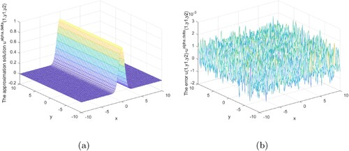
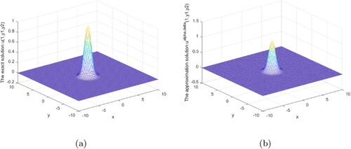
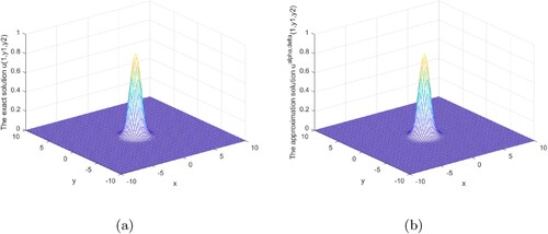
Figures 1–3 show that our regularization method is effective and stable in the interval 0<x<1. Our regularization method is stable and effective at the x = 1 boundary, as shown in Figures 4–6.

Example 5.2

As the exact data for Problem (2.1(2.1) $\{\begin{array}{l}\mathrm{\Delta }w(x,\mathbf{y})+k^{2}w(x,\mathbf{y})=0,0<x<1,\mathbf{y}\in R^n,\\ w(0,\mathbf{y})=\phi (\mathbf{y}),\mathbf{y}\in R^n,\\ w_x(0,\mathbf{y})=\psi (\mathbf{y}),\mathbf{y}\in R^n,\end{array}$(2.1) ), we use function $\phi (y,z)=\mathrm{yz}{e}^{-x^2-y^2}$.

Figure 1. x = 0.1, $\delta =1\times {10}^{-3}$, (a) Exact solution, (b) Regularized solution.

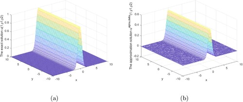
Figure 2. x = 0.2, $\delta =1\times {10}^{-3}$, (a) Regularized solution, (b) Error.

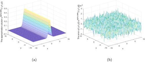
Figure 3. x = 0.5, $\delta =1\times {10}^{-3}$, (a) Regularized solution, (b) Error.

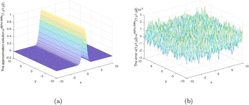
Figure 4. x = 1, p = 0.5, $\delta =1\times {10}^{-3}$, (a) Exact solution, (b) Regularized solution.

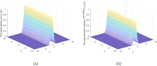
Figure 5. x = 1, p = 3, $\delta =1\times {10}^{-3}$, (a) Regularized solution, (b) Error.

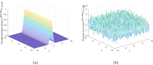
Figure 6. x = 1, p = 5, $\delta =1\times {10}^{-3}$, (a) Regularized solution, (b) Error.

We do the analysis for numerical Example 5.2 under the prior regularization rules and the posterior regularization rules, and the analysis demonstrates the stability and effectiveness of our method. Equations (4.30(4.30) $\Vert \frac{(2\pi {)}^{n/2}}{1+{\mu }^2{\eta }^2}{\hat{\phi }}^{\delta }(\eta )-{\hat{\phi }}^{\delta }(\eta )\Vert =\mathrm{\tau \delta }.$(4.30) ) and (4.31(4.31) $\Vert \frac{(2\pi {)}^{n/2}}{1+{\mu }^2{\eta }^2}{\hat{\psi }}^{\delta }(\eta )-{\hat{\psi }}^{\delta }(\eta )\Vert =\mathrm{\tau \delta }.$(4.31) ) are solved by the dichotomy technique in the posterior regularization rule, where $\tau =1.1$.

Table 5 shows that our method is superior to the method [21], as can be shown. Our method has a less relative error than that in [21], a better approximate effect, and it is more stable. The approach presented in this research is stable for p = 0.5 and p = 3, as shown in Table 6.

Table 5. Comparison between different regular solutions when x = 0.2, p = 0.5.

Wave number k	δ	Dirichlet $\mathrm{rel}(u)$	Posterior $\mathrm{rel}(u)$	Prior $\mathrm{rel}(u)$
1	1×${10}^{-2}$	2.5472	0.6966	0.7429
1	1×${10}^{-3}$	0.2608	0.0724	0.0645
1	1×${10}^{-4}$	0.0380	0.0067	0.0069
1	1×${10}^{-5}$	0.0114	0.0007	0.0007
100	1×${10}^{-2}$	3.0165	0.0752	0.0754
100	1×${10}^{-3}$	0.2899	0.0074	0.0075
100	1×${10}^{-4}$	0.0291	0.0007	0.0008
100	1×${10}^{-5}$	0.0060	0.0007	0.0007

Table 6. The relative error of Example 5.2 when x = 1.

Error level δ	p-norm	Wave number k	Prior $\mathrm{rel}(u)$	Posterior $\mathrm{rel}(u)$
1×${10}^{-2}$	3	100	0.0708	0.0725
1×${10}^{-3}$	3	100	0.0075	0.0073
1×${10}^{-4}$	3	100	0.0007	0.0007
1×${10}^{-5}$	3	100	0.0007	0.0007

A graphs display the exact solution, the approximate solution and the error analysis under the a priori regularization parameter choice rule is shown above. It can be seen from Figures 7 to 10 that our regularization method is stable and efficient under prior rules in the interval 0<x<1. Figures 11 and 12 show our regularization method is stable and efficient at the x=1 boundary.

Figure 7. x = 0, $\delta =1\times {10}^{-3}$, (a) Exact solution, (b) Regularized solution.

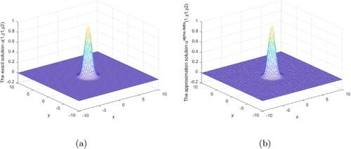
Figure 8. x = 0.2, $\delta =1\times {10}^{-3}$, (a) Regularized solution, (b) Error.

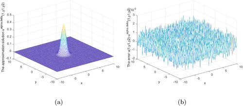
Figure 9. x = 0.5, $\delta =1\times {10}^{-3}$, (a) Regularized solution, (b) Error.

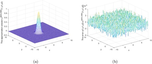
Figure 10. x = 0.8, $\delta =1\times {10}^{-3}$, (a) Regularized solution, (b) Error.

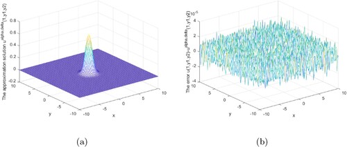
Figure 11. x = 1, p = 0.5, $\delta =1\times {10}^{-3}$, (a) Exact solution, (b) Regularized solution.

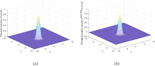
Figure 12. x = 1, p = 3, $\delta =1\times {10}^{-4}$, (a) Regularized solution, (b) Error.

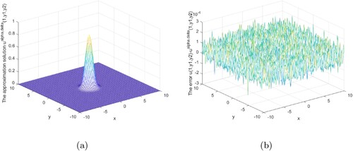
Figure 13. x = 0, $\delta =1\times {10}^{-3}$, (a) Exact solution, (b) Regularized solution.

Figures 13–16 analysis result under the posterior regularization rule is shown above. It can be seen from these graphs that our method is stable and efficient under the posterior rule in the interval or at the boundary.

Figure 14. x = 0.2, $\delta =1\times {10}^{-3}$, (a) Regularized solution, (b) Error.

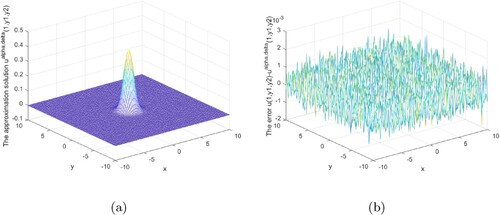
Figure 15. x = 0.5, $\delta =1\times {10}^{-3}$, (a) Regularized solution, (b) Error.

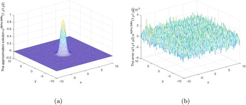
Figure 16. x = 1, p = 0.5, $\delta =1\times {10}^{-4}$, (a) Exact solution, (b) Regularized solution.

6. Conclusion

In this article, we deal with the inverse problem of the multi-dimensional Helmholtz equation by mollification regularization method based on a multi-dimensional exponential decay kernel. The corresponding regular solutions are constructed under the prior rule and posterior rule respectively, and the convergence between the regular and exact solution is proved respectively. Finally, numerical examples are given to demonstrate the effectiveness and stability of the proposed method by combining tables and graphs. From the comparison between the relative errors in Table 5, it can be seen that the regular solution constructed by the method in this paper is closer to the exact solution than that constructed by the method in literature [21]. As can be seen from the data in Tables 2 and 6, our method is applicable not only to small wave numbers but also to large wave numbers. Among them, Table 3 shows that under different values of p, our method is stable and effective no matter under priori rule or posterior rule.

Acknowledgments

We would like to express our sincere gratitude to the referees and editor for their diligent review of our paper and for providing valuable recommendations. Their insightful feedback has greatly improved the quality of our research!

Disclosure statement

No potential conflict of interest was reported by the author(s).

Additional information

Funding

The financial support provided by the National Natural Science Foundation of China (No. 11961054) and the Natural Science Foundation of Ningxia (No. NZ16011).

References

- Klibanov MV. Two classes of inverse problems for partial differential equation. Ann New York Acad Sci. 1992;661(1):93–111. doi: 10.1111/j.1749-6632.1992.tb26036.x
- Tadi M, Nandakumaran AK, Sritharan SS. An inverse problem for Helmholtz equation. Inverse Probl Sci Eng. 2011;19(6):839–854. doi: 10.1080/17415977.2011.556705
- Jin B, Zheng Y. A meshless method for some inverse problems associated with the Helmholtz equation. Comput Methods Appl Mech Engrg. 2006;195(19-22):2270–2288. doi: 10.1016/j.cma.2005.05.013
- Jin B, Rundell W. A tutorial on inverse problems for anomalous diffusion processes. Inverse Probl. 2015;31(3):035003. doi: 10.1088/0266-5611/31/3/035003
- Bao G, Li P, Zhao Y. Stability in the inverse source problem for elastic and electromagnetic waves with multi-frequencies, 2017. Preprint, arXiv: 1703.03890.
- EI Badia A, EI Hajj A. Stability estimates for an inverse source problem of Helmholtz equation from single Cauchy data at a fixed frequency. Inverse Probl. 2013;29(12):125008. doi: 10.1088/0266-5611/29/12/125008
- Bao G, Lin J, Triki F. Numerical solution of the inverse source problem for the Helmholtz equation with multiple frequency data. Contemp Math. 2011;548:45–60. doi: 10.1090/conm/548
- Zhang D, Guo Y. Fourier method for solving the multi-frequency inverse source problem for the Helmholtz equation. Inverse Probl. 2015;31(3):035007. doi: 10.1088/0266-5611/31/3/035007
- Wang X, Guo Y, Zhang D, et al. Fourier method for recovering acoustic sources from multi-frequency far-field data. Inverse Probl. 2017;33(3):035001. doi: 10.1088/1361-6420/aa573c
- Wang G, Ma F, Guo Y, et al. Solving the multi-frequency electromagnetic inverse source problem by the Fourier method, 2017. Preprint, arXiv: 1708.00673.
- Colton D, Kress R. Inverse acoustic and electromagnetic scattering theory[M]. Berlin: Springer; 1998.
- Guo Y, Monk P, Colton D. Toward a time domain approach to the linear sampling method. Inverse Probl. 2013;29(9):095016. doi: 10.1088/0266-5611/29/9/095016
- Marin L, Elliot L, Heggs PJ, et al. BEM solution for the Cauchy problem associated with Helmholtz-type equations by the Landweber method. Eng Anal Bound Elem. 2004;28:1025–1034. doi: 10.1016/j.enganabound.2004.03.001
- Kirsch A. An introduction to the mathematical theory of inverse problems. 2nd ed. New York: Springer; 2011. (Mathematical sciences).
- Manselli P, Miller K. Calculation of the surface temperature and heat flux on one side of a wall from measurements on the opposite side. Ann Mat Pura Appl. 1980;123(1):161–183. doi: 10.1007/BF01796543
- Murio DA. The mollification method and the numerical solution of ill-Posed problems. John Wiley and Sons Inc; 2011.
- Ha`o DN. A mollification method for ill-posed problems. Numer Math. 1994;68:469–506. doi: 10.1007/s002110050073
- Murio DA. Numerical method for inverse transient heat conduction problems. Rev Unión Mat Argent. 1981;30:25–46.
- Murio DA. On the estimation of the boundary temperature on a sphere from measurements at its center. J Comput Appl Math. 1982;8:111–119. doi: 10.1016/0771-050X(82)90064-X
- He SQ, Feng XF. A regularization method to solve a Cauchy problem for the two-dimensional modified Helmholtz equation. Mathematics. 2019;7:360. doi: 10.3390/math7040360
- Kirsch A. An introduction to the mathematical theory of inverse problems. 2nd ed. Springer; 2011. (Applied mathematical sciences).