Data-driven solutions of ill-posed inverse problems arising from doping reconstruction in semiconductors

ABSTRACT

The non-destructive estimation of doping concentrations in semiconductor devices is of paramount importance for many applications ranging from crystal growth to defect and inhomogeneity detection. A number of technologies (such as LBIC, EBIC and LPS) have been developed which allow the detection of doping variations via photovoltaic effects. The idea is to illuminate the sample at several positions and detect the resulting voltage drop or current at the contacts. We model a general class of such photovoltaic technologies by ill-posed global and local inverse problems based on a drift-diffusion system which describes charge transport in a self-consistent electrical field. The doping profile is included as a parametric field. To numerically solve a physically relevant local inverse problem, we present three approaches, based on least squares, multilayer perceptrons, and residual neural networks. Our data-driven methods reconstruct the doping profile for a given spatially varying voltage signal induced by a laser scan along the sample's surface. The methods are trained on synthetic data sets which are generated by finite volume solutions of the forward problem. While the linear least square method yields an average absolute error around 10%, the nonlinear networks roughly halve this error to 5%.

KEYWORDS:

• Doping reconstruction
• ill-posed inverse problems
• data-driven methods
• photovoltaic technologies

MATHEMATICS SUBJECT CLASSIFICATIONS:

• 65N20
• 65N21
• 35Q81
• 65N08

1. Introduction

Noninvasively estimating doping inhomogeneities in semiconductors is relevant for many industrial applications, ranging from controlling the semiconductor crystal purity during and after growth, the recent redefinition of the 1 kg to detecting defects in the final semiconductor devices such as solar cells. Doping variations lead to local electrical fields. Experimentalists may exploit this mechanism to identify inhomogeneities, variations, and defects in the doping profile by systematically generating electron-hole pairs via some form of electromagnetic radiation. Due to the local fields generated by the doping inhomogeneities, the charge carrier tends to redistribute in the region surrounding the excitation to minimize the energy. The remaining charge carriers will flow through the external circuit, and induce a current which may be measured. By scanning the semiconductor sample with the electromagnetic source at different positions, one can eventually visualize the distribution of electrically active charge-separating defects and variations in the doping profile of the sample along the scan locations.

Several different technologies use the described photovoltage mechanism to analyse doping inhomogeneities. They are classified according to either the type of excitation used to induce the local generation of electron-hole pairs, or the contact placement to measure the generated current, or how the collected signal is related to the doping variation. Electron Beam Induced Current (EBIC) [1], Laser Beam Induced Current (LBIC) [2], scanning photovoltage (SPV) [3], and Lateral Photovoltage Scanning (LPS) [4,5] are some of such photovoltaic technologies, using as electromagnetic sources either localized electron beams (EBIC) or laser beams (LBIC, SPV, and LPS). A typical outcome of these techniques is an image where the intensity of each pixel is proportional to the total current signal induced by a beam shone on the pixel location.

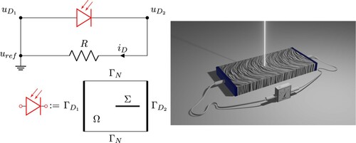
The LPS method, proposed in Refs [4,6] and schematically shown in Figure 1 right panel, is especially useful in the context of crystal growth, where it is virtually impossible to predict the quality (i.e. the symmetry) of a semiconductor crystal during its growth in a furnace. During the growth process, thermal fluctuations near the solid–liquid interface introduce local fluctuations (or striations) in the doping profile. LPS detects such doping inhomogeneities non-invasively at wafer-scale and room temperature. It is especially suitable for low doping concentrations (${10}^{12}{\mathrm{cm}}^{-3}$  to ${10}^{16}{\mathrm{cm}}^{-3}$).

Figure 1. On the top left we show the schematic of a photo-sensitive silicon crystal (in red) coupled with the voltage metre having resistance R (rendered on the right). On the bottom left, we show the domain Ω, the ohmic contacts ${\mathrm{\Gamma }}_{D_1}$ and ${\mathrm{\Gamma }}_{D_2}$, and the laser probing area Σ.

Mathematically speaking, all of the discussed technologies result in inverse problems. The forward problem assumes that we know the doping profile and a set of laser spot positions. We then want to know the corresponding (laser spot dependent) photovoltage signals at the contacts. The inverse problem, on the other hand, assumes we have measured photovoltage signals at the contacts for a laser scan across the sample. Then we want to reconstruct the doping profile at least in the probing region but ideally in the whole domain. We model a general class of photovoltaic technologies introduced above by ill-posed global and local inverse problems based on a drift-diffusion system which describes charge transport in a self-consistent electrical field, the so-called van Roosbroeck system. The doping profile is included as a parametric field. We point out that a key difficulty in the mathematical modelling and numerical simulation is that the probing area where the laser or electron beam operates is significantly smaller (even up to one spatial dimension) than the region in which we would like to recover the doping profile. This means that the solution of such incomplete inverse problems cannot be unique and we have to look for appropriate minimizers or rely on some physically meaningful assumptions on the doping regarding periodicity or variation in only one spatial dimension.

Ill-posed inverse (PDE) problems have been studied for a long time from an analytical and a numerical point of view. We refer to the general overviews [7,8] and the references therein. Burger, Markowich and others analysed inverse semiconductor problems [9,10]. Since the analysis is challenging, they often consider linearized/unipolar settings, no recombination/generation, only small external biases, linear diffusion as well as standard Dirichlet-Neumann boundary conditions. In Ref. [10], they discuss the identifiability of the doping profile from capacitance, reduced current-voltage or laser beam-induced current (LBIC) data. As for the doping reconstruction, previous numerical methods relied on optimization [11], the level set [9] or the Landweber–Kaczmarz methods [10]. Especially, the latter proved to be unstable and costly. For this reason, we propose in this paper data-driven approaches to solve the local inverse photovoltage PDE problem.

In particular, we focus on three data-driven approaches: First, noting that under special conditions the photovoltage signal is related to the doping profile by linear operations, namely differentiation and convolution, we try a classical least squares approach. Second, allowing also a nonlinear relationship between doping profile and photovoltage signal, we train multilayer perceptrons. Finally, we adjust more advanced ResNets to our specific setup to solve the inverse photovoltage problem. Any data-driven technique heavily relies on the amount and quality of the training data. Since, for example, growing crystals is exceptionally costly, we are not able to generate large real-life datasets. For this reason, we generate physics-preserving synthetic data (measured signals and corresponding doping profiles) via a fast and efficient implementation of the forward PDE model [6] which relies on the Voronoi finite volume discretization described in Ref. [12]. As discussed above, in the context of LPS it has been shown that the forward model nicely encompasses three main physically meaningful features [6]. The flux discretization is handled by ideas of Scharfetter and Gummel [13]. Compared to an implementation based on commercial software [14,15], our open-source code reduces the simulation time of the forward model by two orders of magnitude. Finally, we will study the robustness with respect to noise and carefully tune the hyperparameters. We introduce noise in the amplitude as well as in the wave lengths and phase shifts of the doping fluctuations. While the results for noisy data are worse than for clean data, our approach appears to be relatively robust with respect to noise.

The literature on how deep neural networks maybe be used to solve PDEs has been rapidly increasing in recent years. A notable numerical approach is called physics informed neural networks (PINN); see Refs [16] and references therein for more details. The key idea is to replace classical statistical loss functions with PDE residuals. Unfortunately, in our case, this is not directly feasible since solving the forward problem requires knowledge of the doping profile in the entire three-dimensional domain. For the inverse problem, however, the doping profile may only be reconstructed within a two- or even one-dimensional subset. Other approaches include supervised deep learning algorithms [17,18] to efficiently approximate quantities of interest for PDE solutions and [19] and reference therein to accelerate existing PDE numerical schemes. In order to solve high-dimensional PDEs, we refer to Refs [20,21]. In terms of recovering parameters in governing PDEs by solving inverse problems, we refer to Refs [22–26]. In particular, the authors in Ref. [22] consider an inverse scattering problem for nano-optics. How to recover generalized boundary conditions is studied in [23]. Active learning algorithms are also proposed to approximate associated PDE-constrained optimization problems [24]. In Ref. [25], the authors provide model-constrained deep learning approaches for inverse problems. Such strategies are applied in Ref. [26] to reconstruct the second-order coefficients in elliptic problems. Especially in the context of semiconductors, it is often not clear which material parameters such as life times or reference densities are actually correct. For this reason, the authors in Ref. [27] used machine learning techniques to estimate material parameters in the context of organic semiconductors.

The remainder of the paper is organized as follows: In Section 2, we introduce general (forward) PDE models for general electromagnetic source terms and doping profiles based on the van Roosbroeck system which describes charge transport in a self-consistent electrical field. In Section 3, we present global and local inverse photovoltage models for generic electromagnetic source terms. In Section 4, we present the three data-driven approaches we use to solve the local inverse photovoltage problem for a specific LPS setup. We conclude with a summary and an outlook in Section 5.

2. Forward photovoltage model

In this section, we first describe the drift-diffusion charge transport model and then the circuit model which represents the volt metre, modelled by boundary condition. When combining both models, we are able to formulate the forward photovoltage model which may be used to predict a measured signal (either a current or a voltage) for a given doping profile and source of electromagnetic radiation.

2.1. The van Roosbroeck model

The semiconductor crystal is modelled by a bounded domain $\mathrm{\Omega }\subset {\mathbb{R}}^3$ in which two charge carriers evolve: electrons with negative elementary charge $-q$, and holes with positive elementary charge q. The doping profile is given by the difference of donor and acceptor concentrations, $N_D\left(\mathbf{x}\right)-N_A\left(\mathbf{x}\right)=:C\left(\mathbf{x}\right)$, where $\mathbf{x}=(x,y,z{)}^T\in \mathrm{\Omega }$. We assume that C is a bounded function, and we call $\mathcal{C}\subseteq L^{\mathrm{\infty }}\left(\mathrm{\Omega }\right)$ the space of all admissible doping profiles.

We describe the charge transport within the crystal in terms of the electrostatic potential $\psi \left(\mathbf{x}\right)$, and quasi-Fermi potentials for electron and holes, ${\phi }_n\left(\mathbf{x}\right)$ and ${\phi }_p\left(\mathbf{x}\right)$, respectively. The current densities for electrons and holes are given by ${\mathit{J}}_n\left(\mathbf{x}\right)$, ${\mathit{J}}_p\left(\mathbf{x}\right)$. These variables shall satisfy the so-called van Roosbroeck model in which the first equation, a nonlinear Poisson equation is self-consistently coupled with two continuity equations [28] (1) $\begin{array}{ll}-\mathrm{\nabla }\cdot \left(ϵ\mathrm{\nabla \psi }\right)=q(p-n+C(\mathbf{x}\left)\right),& \\ -1/q\mathrm{\nabla }\cdot {\mathit{J}}_n=G(\mathbf{x};{\mathbf{x}}_0)-H,& {\mathit{J}}_n=-q{\mu }_{n}n\mathrm{\nabla }{\phi }_n,\\ 1/q\mathrm{\nabla }\cdot {\mathit{J}}_p=G(\mathbf{x};{\mathbf{x}}_0)-H,& {\mathit{J}}_p=-q{\mu }_{p}p\mathrm{\nabla }{\phi }_p.\end{array}$(1) In the van Roosbroeck model (1(1) $\begin{array}{ll}-\mathrm{\nabla }\cdot \left(ϵ\mathrm{\nabla \psi }\right)=q(p-n+C(\mathbf{x}\left)\right),& \\ -1/q\mathrm{\nabla }\cdot {\mathit{J}}_n=G(\mathbf{x};{\mathbf{x}}_0)-H,& {\mathit{J}}_n=-q{\mu }_{n}n\mathrm{\nabla }{\phi }_n,\\ 1/q\mathrm{\nabla }\cdot {\mathit{J}}_p=G(\mathbf{x};{\mathbf{x}}_0)-H,& {\mathit{J}}_p=-q{\mu }_{p}p\mathrm{\nabla }{\phi }_p.\end{array}$(1) ), the permittivity of the medium is denoted by ε and the mobilities of electrons and holes are respectively indicated by ${\mu }_n$ and ${\mu }_p$. Assuming so-called Boltzmann statistics, the relations between the quasi-Fermi potentials and the densities of electrons and holes, n and p respectively, are given by (2) $n=N_c\exp \left(\frac{q(\psi -{\phi }_n)-E_c}{k_{B}T}\right)\mathrm{and}p=N_v\exp \left(\frac{q({\phi }_p-\psi )+E_v}{k_{B}T}\right).$(2) Here, we have denoted the conduction and valence band densities of states with $N_c$ and $N_v$, the Boltzmann constant with $k_B$ and the temperature with T. Furthermore, $E_c$ and $E_v$ refer to the constant conduction and valence band-edge energies, respectively.

The semiconductor is considered in equilibrium if the quasi-Fermi potentials vanish, ${\phi }_n={\phi }_p=0$. In this case only the nonlinear Poisson equation in (1(1) $\begin{array}{ll}-\mathrm{\nabla }\cdot \left(ϵ\mathrm{\nabla \psi }\right)=q(p-n+C(\mathbf{x}\left)\right),& \\ -1/q\mathrm{\nabla }\cdot {\mathit{J}}_n=G(\mathbf{x};{\mathbf{x}}_0)-H,& {\mathit{J}}_n=-q{\mu }_{n}n\mathrm{\nabla }{\phi }_n,\\ 1/q\mathrm{\nabla }\cdot {\mathit{J}}_p=G(\mathbf{x};{\mathbf{x}}_0)-H,& {\mathit{J}}_p=-q{\mu }_{p}p\mathrm{\nabla }{\phi }_p.\end{array}$(1) ) is solved for the equilibrium electrostatic potential ${\psi }_{\mathrm{eq}}$. The corresponding equilibrium charge carrier densities $n_{\mathrm{eq}}$ and $p_{\mathrm{eq}}$ satisfy $n_{\mathrm{eq}}{p}_{\mathrm{eq}}=n_i^2$, where $n_i$ is the so-called intrinsic carrier density, defined via the relationship $n_i^2=N_c{N}_v\exp (-(E_c-E_v)/k_{B}T)$.

The recombination term H is the sum of the direct recombination, the Auger recombination and the Shockley-Read-Hall recombination, that is respectively: $\begin{array}{rl}{H}_{\mathrm{dir}}& =C_d(\mathrm{np}-n_i^2),H_{\mathrm{Aug}}=C_{n}n(\mathrm{np}-n_i^2)+C_{p}p(\mathrm{np}-n_i^2),\\ H_{\mathrm{SRH}}& =\frac{\mathrm{np}-n_i^2}{{\tau }_p(n+n_T)+{\tau }_n(p+p_T)}.\end{array}$Different types of crystal samples (such as silicon, germanium, gallium arsenide) have different life times ${\tau }_n,{\tau }_p$, and reference densities $n_T,p_T$.

The electromagnetic source (a laser or an electron beam) is modelled by the generation term $G(\mathbf{x};{\mathbf{x}}_0)$. When the laser hits the crystal at the point ${\mathbf{x}}_0:=(x_0,y_0,z_0{)}^T$, some photons are impinged and create electron-hole pairs, resulting in a generation rate defined as follows (3) $G(\mathbf{x};{\mathbf{x}}_0)=\mathrm{\kappa S}(\mathbf{x}-{\mathbf{x}}_0),$(3) where $S\left(\mathbf{x}\right)$ is the shape function of the laser (normalized by ${\int }_{{\mathbb{R}}^3}S\left(\mathbf{x}\right)d\mathbf{x}=1$), while κ is a constant given by $\kappa :=\frac{P{\lambda }_L}{h}(1-r)$. Here, P is the laser power, ${\lambda }_L$ is the wave length of the laser, h is the Planck constant, and r is the reflectivity rate of the crystal.

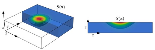
We assume that the area of influence of the electromagnetic source decays exponentially fast from the incident point ${\mathbf{x}}_0$. In particular, we take a laser profile function S defined as (4) $S\left(\mathbf{x}\right):=\frac{1}{2\pi {\sigma }_L^2{d}_A}\exp [-\frac{1}{2}{\left(\frac{x}{{\sigma }_L}\right)}^2]\exp [-\frac{1}{2}{\left(\frac{y}{{\sigma }_L}\right)}^2]\exp [-\frac{|z|}{d_A}].$(4) Here ${\sigma }_L$ is the laser spot radius, while $d_A$ is the penetration depth (or the reciprocal of the absorption coefficient), which heavily depends on the laser wave length. Figure 2 shows a typical configuration, where the laser beam hits the crystal on the top surface, and shows the exponential decay of the laser shape function S.

Figure 2. A zoom-in of the area around the point ${\mathbf{x}}_0$, where the laser hits the crystal (left), and a cross-section of the device at y = 0 used in the 2D simulation (right).

A prototypical setting for photovoltage measurements is given by a cuboid sample attached to a voltmeter with resistance R, and the electromagnetic source aiming at its top surface.

2.2. Boundary conditions

The PDE system (1(1) $\begin{array}{ll}-\mathrm{\nabla }\cdot \left(ϵ\mathrm{\nabla \psi }\right)=q(p-n+C(\mathbf{x}\left)\right),& \\ -1/q\mathrm{\nabla }\cdot {\mathit{J}}_n=G(\mathbf{x};{\mathbf{x}}_0)-H,& {\mathit{J}}_n=-q{\mu }_{n}n\mathrm{\nabla }{\phi }_n,\\ 1/q\mathrm{\nabla }\cdot {\mathit{J}}_p=G(\mathbf{x};{\mathbf{x}}_0)-H,& {\mathit{J}}_p=-q{\mu }_{p}p\mathrm{\nabla }{\phi }_p.\end{array}$(1) ) is supplemented with Dirichlet and Neumann boundary conditions. The boundary $\mathrm{\partial \Omega }$ is the union of two disjoint parts ${\mathrm{\Gamma }}_N$ and ${\mathrm{\Gamma }}_D$. On ${\mathrm{\Gamma }}_N$, we assign Neumann boundary conditions (5) $\frac{\mathrm{\partial }\psi }{\mathrm{\partial }\mathit{\nu }}=\frac{\mathrm{\partial }{\phi }_n}{\mathrm{\partial }\mathit{\nu }}=\frac{\mathrm{\partial }{\phi }_p}{\mathrm{\partial }\mathit{\nu }}=0,$(5) where $\mathrm{\partial }/\mathrm{\partial }\mathit{\nu }=\mathit{\nu }\cdot \mathrm{\nabla }$ is the normal derivative along the external unit normal $\mathit{\nu }$. On ${\mathrm{\Gamma }}_D$, we assign Dirichlet-type boundary conditions. This type of boundary condition models so-called ohmic contacts [29]. We suppose that there are two ohmic contacts, i. e. ${\mathrm{\Gamma }}_D={\mathrm{\Gamma }}_{D_1}\cup {\mathrm{\Gamma }}_{D_2}$. The ohmic boundary conditions can be summarized by (6) $\psi -{\psi }_0={\phi }_n={\phi }_p=u_{D_i}-u_{\mathrm{ref}}\mathrm{on}{\mathrm{\Gamma }}_{D_i},i=1,2,$(6) where ${\psi }_0$ is the local electroneutral potential which one obtains by solving the Poisson equation for ψ for a vanishing left-hand side. The terms $u_{D_i}$ denote the contact voltages at the corresponding ohmic contacts; for the forward model their difference is a priori unknown. We define a reference value $u_{\mathrm{ref}}$ of the potential and set it to $u_{\mathrm{ref}}=0=u_{D_1}$.

The total electric current $i_D$ flowing through the ohmic contact ${\mathrm{\Gamma }}_{D_2}$ is defined by the surface integral (7) $\begin{array}{rl}{i}_D:\mathrm{\Omega }\times \mathbb{R}\times \mathcal{C}& \to \mathbb{R}\\ ({\mathbf{x}}_0,u_{D_2},C)& \mapsto i_D({\mathbf{x}}_0,u_{D_2},C):={\int }_{{\mathrm{\Gamma }}_{D_2}}\mathit{\nu }\cdot \left({\mathit{J}}_n\right(\mathbf{x})+{\mathit{J}}_p(\mathbf{x}\left)\right)\mathrm{d}\sigma \left(\mathbf{x}\right).\end{array}$(7) The current $i_D$ is a function of the contact voltage $u_{D_2}$, of the laser spot position ${\mathbf{x}}_0$, and of the doping profile C.

In order to close the system, we model the voltage/ampere metre as a simple circuit having a resistance R. This structure is visualized in Figure 1. When the external circuit is connected to the crystal, the boundary condition $u_{D_2}$ can no longer be chosen arbitrarily and must balance the voltage difference at the voltmeter due to the current $i_D$, which is equal to the product $R{i}_D$. A generalized theory of this coupling can be found in Ref. [30] and in the references therein.

Let $\mathcal{U}$ be the function space of all possible photovoltage signals as a function of the laser spot position ${\mathbf{x}}_0$ that can be measured at the contacts for any given admissible doping profile $C\in \mathcal{C}$. We define the laser-voltage (L-V) map as precisely the map that associates to each laser spot location ${\mathbf{x}}_0$ and doping profile C the corresponding photovoltage signal $u_P$ which satisfies the second ohmic boundary condition in (6(6) $\psi -{\psi }_0={\phi }_n={\phi }_p=u_{D_i}-u_{\mathrm{ref}}\mathrm{on}{\mathrm{\Gamma }}_{D_i},i=1,2,$(6) ) and balances the voltage difference across R, that is (8) $\begin{array}{rl}{u}_P:\mathrm{\Omega }\times \mathcal{C}& \to \mathbb{R}\\ ({\mathbf{x}}_0,C)& \mapsto u\in \mathcal{U}\mathrm{such}\mathrm{that}u\left({\mathbf{x}}_0\right)-R{i}_D({\mathbf{x}}_0,u,C)=0\mathrm{and}u\left({\mathbf{x}}_0\right)=u_{D_2}.\end{array}$(8) The laser-voltage map (8(8) $\begin{array}{rl}{u}_P:\mathrm{\Omega }\times \mathcal{C}& \to \mathbb{R}\\ ({\mathbf{x}}_0,C)& \mapsto u\in \mathcal{U}\mathrm{such}\mathrm{that}u\left({\mathbf{x}}_0\right)-R{i}_D({\mathbf{x}}_0,u,C)=0\mathrm{and}u\left({\mathbf{x}}_0\right)=u_{D_2}.\end{array}$(8) ) corresponds to a nonlinear version of Ohm's law at the contact and constitutes an implicit equation for the Dirichlet boundary condition $u_{D_2}$ of the van Roosbroeck system (1(1) $\begin{array}{ll}-\mathrm{\nabla }\cdot \left(ϵ\mathrm{\nabla \psi }\right)=q(p-n+C(\mathbf{x}\left)\right),& \\ -1/q\mathrm{\nabla }\cdot {\mathit{J}}_n=G(\mathbf{x};{\mathbf{x}}_0)-H,& {\mathit{J}}_n=-q{\mu }_{n}n\mathrm{\nabla }{\phi }_n,\\ 1/q\mathrm{\nabla }\cdot {\mathit{J}}_p=G(\mathbf{x};{\mathbf{x}}_0)-H,& {\mathit{J}}_p=-q{\mu }_{p}p\mathrm{\nabla }{\phi }_p.\end{array}$(1) ). An existence result for solutions of the laser-voltage map is provided in Ref. [31], with the assumption that the generation rate G is small enough. For a spatially varying doping profile C, the laser-voltage map $u_P({\mathbf{x}}_0,C)$ may be different for each laser spot location ${\mathbf{x}}_0$.

2.3. The global forward photovoltage problem

Although the presented forward PDE model is well-posed for low laser power intensity and for all laser spot positions ${\mathbf{x}}_0\in \mathrm{\Omega }$, not all positions in Ω can be illuminated by a laser. The major limiting factor is the fact that the laser power intensity decays exponentially away from the surface of the crystal sample, leaving in fact as the only feasible positions those that are near or on the surface of the crystal sample.

We denote with $\mathrm{\Sigma }\subseteq \overline{\mathrm{\Omega }}$ the set of all admissible laser spot positions ${\mathbf{x}}_0$. Our global forward photovoltage problem then associates to each doping profile C the function u that maps each laser spot position ${\mathbf{x}}_0\in \mathrm{\Sigma }$ to the corresponding photovoltage signal $u_P({\mathbf{x}}_0,C)$, i.e. (9) $\begin{array}{rl}U:\mathcal{C}& \to \mathcal{U}\\ C& \mapsto u:\mathrm{\Sigma }\to \mathbb{R},u\left({\mathbf{x}}_0\right)=u_P({\mathbf{x}}_0,C),{\mathbf{x}}_0\in \mathrm{\Sigma }.\end{array}$(9)

3. Inverse photovoltage problems

From an industrial perspective, more interesting than the forward photovoltage problem is the inverse one. How do doping inhomogeneities influence the measured voltage difference $u_P$, defined in the previous section? Suppose we have measured the photovoltage signal for several different laser spot positions ${\mathbf{x}}_0$, how does the doping profile look like that leads to this signal? Since the doping profile enters as a volumetric source term defined in the whole domain in the van Roosbroeck system (1(1) $\begin{array}{ll}-\mathrm{\nabla }\cdot \left(ϵ\mathrm{\nabla \psi }\right)=q(p-n+C(\mathbf{x}\left)\right),& \\ -1/q\mathrm{\nabla }\cdot {\mathit{J}}_n=G(\mathbf{x};{\mathbf{x}}_0)-H,& {\mathit{J}}_n=-q{\mu }_{n}n\mathrm{\nabla }{\phi }_n,\\ 1/q\mathrm{\nabla }\cdot {\mathit{J}}_p=G(\mathbf{x};{\mathbf{x}}_0)-H,& {\mathit{J}}_p=-q{\mu }_{p}p\mathrm{\nabla }{\phi }_p.\end{array}$(1) ), but we can only probe part of the domain with the laser signal, answering such a question implies solving an ill-posed inverse problem: different global doping profiles may lead to the same signal. Hence, we will first formulate an idealized global inverse photovoltage problem and then a practically relevant local inverse photovoltage problem.

3.1. Global inverse photovoltage problem

Ideally, we would like to find the global doping reconstruction operator $\tilde{F}:=U^{-1}:\mathcal{U}\to \mathcal{P}\left(\mathcal{C}\right),$that, for a given photovoltage signal measurement u, returns the preimage $U^{-1}\left(u\right)$. Here we indicate with $\mathcal{P}\left(\mathcal{C}\right)$ the power set of $\mathcal{C}$, i.e. the set of all possible subsets of $\mathcal{C}$. The global inverse photovoltage problem reads (10) $\tilde{F}\left(u\right)={\mathcal{C}}_u,{\mathcal{C}}_u:=\{C\in \mathcal{C}\mathrm{such}\mathrm{that}{u}_P(\cdot ,C)=u\},$(10) that is, $\tilde{F}$ is a function from $\mathcal{U}$ to $\mathcal{P}\left(\mathcal{C}\right)$ (i.e. a multi-valued function of the signal u) such that $C\subseteq \tilde{F}\left(u_P\right(\cdot ,C\left)\right)$ for all $C\in \mathcal{C}$.

3.2. Local inverse photovoltage problem

In practice, however, the construction of the operator $\tilde{F}$ (even the construction of an approximation of $\tilde{F}$) is nontrivial, and we would like to simplify our problem by building a local inverse problem that is better posed. A key point when defining a local inverse problem, is the fact that we cannot probe the entire domain Ω with the laser, but only the subset of all possible laser spot positions Σ near or on the surface of Ω. In the following subsections, we will make some assumptions on the structure of technologically feasible doping profiles. Technological feasibility depends on the growth process, on the technology used to inject doping in the crystal, and on the specific photovoltage technology. Here, we assume variation only in the x-direction. That is, $C\left(\mathbf{x}\right)=C\left(x\right)$. This class of doping profiles is relevant, for example, for crystal growth, where striations in the doping profile indicate fluctuations of the temperature field during the growth process, which are dominant in the growth direction.

We define the set of technologically feasible (TF) doping profiles and the set of corresponding signals as (11) ${\mathcal{C}}_{\mathrm{TF}}=\{C\in \mathcal{C}\mathrm{such}\mathrm{that}C(\mathbf{x})=C(x\left)\right\},{\mathcal{U}}_{\mathrm{TF}}:=u_P(\cdot ,{\mathcal{C}}_{\mathrm{TF}}).$(11) With these assumptions on the doping profile, it is reasonable to presume that the photovoltage signal will be influenced more by variations of the doping profile in the vicinity of the laser spot position, which is where most of the charge carriers are generated, and therefore we define the local inverse photovoltage problem by restricting the global inverse problem (10(10) $\tilde{F}\left(u\right)={\mathcal{C}}_u,{\mathcal{C}}_u:=\{C\in \mathcal{C}\mathrm{such}\mathrm{that}{u}_P(\cdot ,C)=u\},$(10) ) both in terms of technologically feasible doping profiles, as well as in terms of probing domain: (12) $F\left(u\right):=\left(\tilde{F}\right(u)\cap {\mathcal{C}}_{\mathrm{TF}}){|}_{\mathrm{\Sigma }}=({\mathcal{C}}_u\cap {\mathcal{C}}_{\mathrm{TF}}){|}_{\mathrm{\Sigma }}=:{\mathcal{C}}_{\mathrm{TF},u,\mathrm{\Sigma }},$(12) where the restriction operator $|$ is applied to each element in the set. The goal of the local inverse problem is to reconstruct doping profiles only in the probing area Σ and not on the whole domain Ω. However, the underlying assumption is that the local doping reconstruction will give us information in a neighbourhood of Σ, or even on all of Ω, when one makes additional assumptions (for example on doping periodicity). In general, the set ${\mathcal{C}}_{\mathrm{TF},u,\mathrm{\Sigma }}=F\left(u\right)$ is much smaller than the set ${\mathcal{C}}_u:=\tilde{F}\left(u\right)$, since it restricts the family of admissible doping profiles to ${\mathcal{C}}_{\mathrm{TF}}$, and discards all of the information outside of Σ. Two doping profiles in ${\mathcal{C}}_u$ correspond to the same element in ${\mathcal{C}}_{\mathrm{TF},u,\mathrm{\Sigma }}$ as soon as their restrictions on Σ coincide.

In principle, it should be possible to formulate a well-posed local inverse problem by further reducing the admissible doping profiles ${\mathcal{C}}_{\mathrm{TF}}$ until the set ${\mathcal{C}}_{\mathrm{TF},u,\mathrm{\Sigma }}$ contains just one single element for any admissible input signal $u\in U\left({\mathcal{C}}_{\mathrm{TF}}\right)$. We do not know, however, if this procedure is feasible, and what the necessary and sufficient conditions on ${\mathcal{C}}_{\mathrm{TF}}$ and on Σ are to ensure that the local inverse problem $F\left(u\right)$ is well-posed. We leave these questions for future investigations and concentrate on numerical approximations of the local inverse problem based on well-posed finite dimensional approximations of $F$. In Section 4, we propose three different strategies (of increasing complexity) to build an approximate inverse operator $F_h$ starting from a collection of doping profiles restricted to a discrete set of probing points ${\mathrm{\Sigma }}_h$ and their corresponding discrete photovoltage signals.

Remark 3.1

The numerical approximations that we construct always produce a unique answer for each finite sampling of a signal u in ${\mathcal{U}}_{\mathrm{TF}}$. We do not attempt to construct the full set ${\mathcal{C}}_{\mathrm{TF},u,\mathrm{\Sigma }}$ of all possible doping profiles that would generate u, but only provide the sampling of a single doping profile C, which is, in some sense, a representative of the set ${\mathcal{C}}_{\mathrm{TF},u,\mathrm{\Sigma }}$. The ill-posedness of the local inverse problem and the impossibility to recover the full doping profile C after having solved the approximate inverse problem is one of the reasons why we cannot use more modern techniques (such as Physics-Informed Neural Networks (PINN) [16]) that would exploit the residual of the forward problem to improve the construction of an approximate inverse operator.

4. Data-driven approximation of the inverse photovoltage problem

Inverse problems for charge transport equations have often been tackled with standard techniques (see, for example, Refs [9–11]). However, in other fields such as image recognition or weather prediction, data-driven approaches have gained significant momentum to solve a variety of inverse problems (see, for example, Refs [32–34]).

In order to formulate a data-driven approach for the numerical approximation of the operator $F$, we leverage the well-posedness of the forward problem $U$ and its discrete approximation described in Ref. [6] to formulate a discrete inverse problem $F_h$ as a well-posed minimization problem in a finite-dimensional space.

4.1. Discrete local inverse problem

Let $\mathrm{\Sigma }\subseteq \overline{\mathrm{\Omega }}$ be a subdomain. We assume we sampled both the photovoltage signal $u_P$ and the doping profile C at $n\in \mathbb{N}$ discrete laser spot positions which shall be contained in the discrete mesh ${\mathrm{\Sigma }}_h\subseteq \mathrm{\Sigma }$. With the boldface symbols $\mathbf{u}$ and $\mathbf{C}$, we indicate the discrete samplings of the signal $u_P(\cdot ,C)$ and the doping profile C evaluated on ${\mathrm{\Sigma }}_h$, respectively. Notice that the generation of a single pair of signal and doping samples $(\mathbf{u},\mathbf{C})\in {\mathbb{R}}^{n\times 2}$ from an admissible doping profile $C\in {\mathcal{C}}_{\mathrm{TF}}$ requires in fact the solution of n discrete van Roosbroeck systems (1(1) $\begin{array}{ll}-\mathrm{\nabla }\cdot \left(ϵ\mathrm{\nabla \psi }\right)=q(p-n+C(\mathbf{x}\left)\right),& \\ -1/q\mathrm{\nabla }\cdot {\mathit{J}}_n=G(\mathbf{x};{\mathbf{x}}_0)-H,& {\mathit{J}}_n=-q{\mu }_{n}n\mathrm{\nabla }{\phi }_n,\\ 1/q\mathrm{\nabla }\cdot {\mathit{J}}_p=G(\mathbf{x};{\mathbf{x}}_0)-H,& {\mathit{J}}_p=-q{\mu }_{p}p\mathrm{\nabla }{\phi }_p.\end{array}$(1) ), one for each laser spot position ${\mathbf{x}}_0\in {\mathrm{\Sigma }}_h$.

The local discrete inverse problem $F_h$ can be interpreted as a (generally nonlinear) function that maps a vector of signal measurements $\mathbf{u}\in {\mathbb{R}}^n$ to a vector of doping profile values $\mathbf{C}\in {\mathbb{R}}^n$: (13) $\begin{array}{rl}{F}_h:{\mathbb{R}}^n& \to {\mathbb{R}}^n\\ \mathbf{u}& \mapsto \mathbf{C}.\end{array}$(13) Ideally, we would like to build $F_h$ in such a way that for all u in ${\mathcal{U}}_{\mathrm{TF}}$, there exists a $C\in {\mathcal{C}}_{\mathrm{TF},u,\mathrm{\Sigma }}=F\left(u\right)$ such that $F_h(\mathbf{u}:=u{|}_{{\mathrm{\Sigma }}_h})=\mathbf{C}:=C{|}_{{\mathrm{\Sigma }}_h}$. However, this procedure suffers from the non-uniqueness of $F\left(u\right)$, which we mitigate by constructing $F_h$ through a well-posed minimization problem.

In practice, we build $F_h$ by minimizing the mean square error loss (14) $\mathrm{MSE}\left(\right\{{\mathbf{u}}_j,{\mathbf{C}}_j{\}}_{j=1}^{N_{\mathrm{train}}}):=\frac{1}{N_{\mathrm{train}}}\sum _{j=1}^{N_{\mathrm{train}}}\Vert F_h\left({\mathbf{u}}_j\right)-{\mathbf{C}}_j{\Vert }_{{\ell }^2}^2,$(14) on a given training dataset $\{{\mathbf{u}}_j,{\mathbf{C}}_j{\}}_{j=1}^{N_{\mathrm{train}}}$ consisting of a collection of $N_{\mathrm{train}}$ pairs of signal samples ${\mathbf{u}}_j$ and doping samples ${\mathbf{C}}_j$. The generation process of the data is detailed in Section 4.3.

The quality of the approximation of $F_h$ is evaluated by measuring the prediction capabilities of $F_h$ on a test dataset that is independent of the training dataset. For the evaluation of the prediction quality, we use the ${\ell }^{\mathrm{\infty }}$ norm and define the test error as (15) $\mathrm{TE}\left(\right\{{\mathbf{u}}_j,{\mathbf{C}}_j{\}}_{j=1}^{N_{\mathrm{test}}}):=\frac{1}{N_{\mathrm{test}}}\sum _{j=1}^{N_{\mathrm{test}}}\Vert F_h\left({\mathbf{u}}_j\right)-{\mathbf{C}}_j{\Vert }_{{\ell }^{\mathrm{\infty }}}.$(15) It is worth noting that, while the definition of the $\mathrm{MSE}$ function relies on the ${\ell }^2$ norm, in Equation  (15(15) $\mathrm{TE}\left(\right\{{\mathbf{u}}_j,{\mathbf{C}}_j{\}}_{j=1}^{N_{\mathrm{test}}}):=\frac{1}{N_{\mathrm{test}}}\sum _{j=1}^{N_{\mathrm{test}}}\Vert F_h\left({\mathbf{u}}_j\right)-{\mathbf{C}}_j{\Vert }_{{\ell }^{\mathrm{\infty }}}.$(15) ) we are using the ${\ell }^{\mathrm{\infty }}$ norm. There are several reasons for this. First of all, minimizing the ${\ell }^{\mathrm{\infty }}$ error is more difficult than minimize the ${\ell }^2$ error; therefore, when we build our models, we take advantage of the smoothness of the ${\ell }^2$ norm. But the ${\ell }^{\mathrm{\infty }}$ error has several advantages: its independence from the size of the domain and its physical meaning of being an upper bound for the pointwise error.

On the other hand, the ${\ell }^{\mathrm{\infty }}$ error has several advantages: it is independent of the size of the domain and it has the physical meaning of being an upper bound on the error on each point. Finally, we perform some hyperparameter tuning on our models (i.e. given a family of models, we choose the one that performs better; see Sections 4.5 and 4.6). Since we generate our models by minimizing the ${\ell }^2$ error while the tuning of the hyperparameters minimizes the error in ${\ell }^{\mathrm{\infty }}$, we keep both of them under control (and therefore, by interpolation, we control every other error in ${\ell }^k$ for $k\ge 2$). Indeed, the training of a specific model minimizes the ${\ell }^2$ error without taking into account the effect this procedure has in the ${\ell }^{\mathrm{\infty }}$ space; on the other hand, if this effect is too detrimental for the ${\ell }^{\mathrm{\infty }}$ error, we discard that model during the tuning of the hyperparameters.

We develop three approaches to build $F_h$:

• Least squares (LS): we approximate $F_h\left(\mathbf{u}\right)$ by the matrix vector product of an $n\times n$ matrix ${\mathbf{A}}_h$ with $\mathbf{u}$. We find the matrix by minimizing the MSEL error defined in (14(14) $\mathrm{MSE}\left(\right\{{\mathbf{u}}_j,{\mathbf{C}}_j{\}}_{j=1}^{N_{\mathrm{train}}}):=\frac{1}{N_{\mathrm{train}}}\sum _{j=1}^{N_{\mathrm{train}}}\Vert F_h\left({\mathbf{u}}_j\right)-{\mathbf{C}}_j{\Vert }_{{\ell }^2}^2,$(14) ) over all $n\times n$ matrices;

• Multilayer perceptron (MLP): we approximate $F_h\left(\mathbf{u}\right)$ by a multilayer perceptron, and use Stochastic Gradient Descent (SGD) to minimize the MSE;

• Residual neural network (ResNet): we approximate $F_h\left(\mathbf{u}\right)$ by a residual neural network, and use SGD to minimize the MSE.

4.2. An industrial application: the LPS setup

We introduce a specific LPS setup for a silicon sample, discuss how and why we generate the data from the forward model as well as solve the corresponding local inverse photovoltage problem via the three data-driven approaches introduced in Section 4.1.

We consider a silicon cuboid of the form $\mathrm{\Omega }:=[-\ell /2,\ell /2]\times [-w/2,w/2]\times [-h,0]$ with length $\ell =3\mathrm{mm}$, width $w=0.5\mathrm{mm}$ and height $h=5\times {10}^{-5}\mathrm{mm}$, ohmic contacts at $x=-\ell /2$ (corresponding to ${\mathrm{\Gamma }}_{D_1}$) and $x=\ell /2$ (corresponding to as ${\mathrm{\Gamma }}_{D_2}$), see Figure 1. We focus on a lateral photovoltage scanning (LPS) table-top setup, see Figure 1 right panel. The silicon parameters needed for the corresponding forward model from Section 2 can be found in Ref. [6]. We simulate the charge transport in the two-dimensional plane where y = 0 and reconstruct the doping profile along a line, namely the subdomain $\mathrm{\Sigma }=\left\{\right(x,0,0{)}^T\in \mathrm{\Omega }:x\in [0,k/2]\}$ with $k<\ell$, ensuring we are sufficiently far away from the boundaries $x=\pm \ell /2$ to reduce boundary effects. The laser scan then produces a uniform partition $0=x_1<\dots <x_n=k/2$ with mesh size $\mathrm{\Delta x}$. The resulting laser spot positions are given by ${\mathrm{\Sigma }}_h:=\{{\mathbf{x}}_i{\}}_{i=1}^n=\{(x_i,0,0{)}^T{\}}_{i=1}^n$. In the following numerical simulations, we set n = 1200 and $k=0.4\mathrm{mm}$.

4.3. Data generation

For our data-driven approaches, we need a suitable amount of data; unfortunately, generating enough data from real life requires large budgets. Instead, we will generate synthetic data from the forward model that we have described in Section 2. These data are physically meaningful in the sense that our finite volume approximation of the LPS problem correctly incorporates physically meaningful behaviour, namely (i) the signal intensity depends linearly on local doping variations for low laser powers, (ii) the signal saturates for higher laser intensities due to a screening effect, and (iii) the signal depends logarithmically on moderate laser intensities [6].

As pointed out in Section 3.2, we consider a family of doping profiles that vary only along the x direction, and that are constant in both y and z directions. To generate our synthetic datasets, we need an algorithm that produces fluctuating doping profiles. Since within the LPS framework, the doping profile is roughly periodic, see Ref. [6], we assume a superposition of sinusoidal functions from which we randomly sample physically reasonable amplitudes and wavelengths. Therefore, we define (16) $C(\mathbf{x}=(x,y,z{)}^T;\text{β}=(C_0,\mathit{\alpha },\mathit{\lambda }{)}^T)=C_0(1+\sum _{i=1}^{N_b}{\alpha }_{i}n\frac{2\mathrm{\pi x}}{{\lambda }_i}),$(16) where $\text{β}$ is a vector of parameters that includes a fixed average doping value $C_0=1.0\times {10}^{16}{\mathrm{cm}}^{-3}$ (a typical value for silicon crystals), amplitudes $\mathit{\alpha }:=\left\{{\alpha }_i\right\}\subset \left\{0\right\}\cup [0.05,0.2]$, and wavelengths $\mathit{\lambda }:=\left\{{\lambda }_i\right\}\subset [10\mathrm{\mu m},1000\mathrm{\mu m}]$. In our simulation, we set the number of sine terms to $N_b=5$, which seems to strike a good balance between complexity and real-life situations for striations in doping profiles.

To generate an element $\{\mathbf{u},\mathbf{C}\}$ of our dataset, we randomly sample a parameter $\text{β}$ with which we generate a continuous function $C(\mathbf{x},\text{β})$ and we compute the discrete counterpart of $u:=U\left(C\right)$ defined in Equation  (9(9) $\begin{array}{rl}U:\mathcal{C}& \to \mathcal{U}\\ C& \mapsto u:\mathrm{\Sigma }\to \mathbb{R},u\left({\mathbf{x}}_0\right)=u_P({\mathbf{x}}_0,C),{\mathbf{x}}_0\in \mathrm{\Sigma }.\end{array}$(9) ) using the finite volume scheme developed in Ref. [35]. Finally, we restrict both C and u to the discrete laser spot mesh ${\mathrm{\Sigma }}_h$.

In realistic physical scenarios, the doping profiles contain noises, and they cannot be represented exactly by Equation  (16(16) $C(\mathbf{x}=(x,y,z{)}^T;\text{β}=(C_0,\mathit{\alpha },\mathit{\lambda }{)}^T)=C_0(1+\sum _{i=1}^{N_b}{\alpha }_{i}n\frac{2\mathrm{\pi x}}{{\lambda }_i}),$(16) ). To simulate such scenario, we perturb some of the doping profiles and generate an additional noisy dataset, used to test the robustness of our networks in the presence of noise. In what follows, we say that a dataset is “noisy” or “clean” if C has or has not been perturbed. The algorithm used to generate noisy datasets is described in Appendix 1.

In the following, we summarize the datasets used to construct and test the learning models introduced in Section 4.4–4.6. The datasets are available on the repository [36].

CleanDataSET

Consisting of:

• CleanTrainingDataSET: a dataset with $N_{\mathrm{train}}=22,500$ clean samples used to train our initial model;

• CleanTestDataSET: a dataset with $N_{\mathrm{test}}=7,500$ clean samples. With this dataset, we test the performance of our models trained by CleanTrainingDataSET. Note that testing errors generated by this dataset (cf. (15(15) $\mathrm{TE}\left(\right\{{\mathbf{u}}_j,{\mathbf{C}}_j{\}}_{j=1}^{N_{\mathrm{test}}}):=\frac{1}{N_{\mathrm{test}}}\sum _{j=1}^{N_{\mathrm{test}}}\Vert F_h\left({\mathbf{u}}_j\right)-{\mathbf{C}}_j{\Vert }_{{\ell }^{\mathrm{\infty }}}.$(15) )) implies the quality of a trained model. This will help use tune the corresponding hyperparameters;

• CleanValidationDataSET: a dataset with the same size of the CleanTestDataSET that will be used to validate the performance of our model on the clean case after performing the tuning.

NoisyDataSET Consisting of:

• NoisySmallTestDataSET: again a dataset of $N_{\mathrm{test}}=7,500$ samples, but this time with noise. This is used to test the robustness of the models trained by the CleanTestDataSET;

• NoisyTrainingDataSET: a dataset with $N_{\mathrm{train}}=150,000$ noisy samples that we use to train our models to be robust to noise;

• NoisyTestDataSET: a dataset with $N_{\mathrm{test}}=50,000$ noisy samples. This is the dataset that we use to test the performances of our models trained with the NoisyTrainingDataSET.

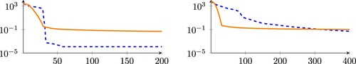
We provide a qualitative analysis of CleanTrainingDataSET and NoisyTrainingDataSET in Figure 3, where we compute the Singular Value Decomposition (SVD) of both datasets interpreted as $n\times N_{\mathrm{train}}$ matrices. The number of dominant singular values is a crude indication of the actual dimension of the spaces ${\mathcal{C}}_{\mathrm{TF}}$, and ${\mathcal{U}}_{\mathrm{TF}}$, and shows that, roughly, their dimension is close to 50 when using the clean data generation described above, see Figure 3 left panel. The two dimensions mismatch significantly when adding noise, see Figure 3 right panel. While the dimension of the clean photovoltage signals follows roughly that of the clean doping profiles, the same cannot be said for the noisy cases. This difference is a hint that the inverse operator $F$ is not well-posed, due to a mismatch in the dimension of the input and output spaces.

Figure 3. SVD analysis of CleanTrainingDataSET and NoisyTrainingDataSET. The figure shows the magnitude of the first 200 singular values for CleanTrainingDataSET (left) and the first 400 singular values for NoisyTrainingDataSET. The singular values for the doping profile matrices are shown in dashed blue lines and the singular values for the photovoltage signals are shown as solid orange lines.

4.4. Least squares

In Ref. [6], the authors showed that, under certain restrictive conditions, the operator $F$ can be approximated by a linear one. Indeed, in case of an n or p doped semiconductor that varies only along the x direction, we can show that (17) $u_P(\mathbf{x},C)m-{\mathbf{e}}_x\cdot \mathrm{\nabla C}\left(\mathbf{x}\right).$(17) If the support of the laser source is larger than the wavelength of oscillation of the doping profile, measuring the voltage difference may actually result in a signal that does not capture a single oscillation, but a floating average. We could represent this floating average of doping fluctuations by a convolution of the doping gradient with some (unknown) profile f, i.e.  (18) $u_P(x,C)m(f\ast ({\mathbf{e}}_x\cdot \mathrm{\nabla C}\left)\right)\left(x\right)=\frac{\mathrm{d}}{\mathrm{d}x}(f\ast C)\left(x\right).$(18) Hence, it may seem plausible to relate the photovoltage signal to the doping profile via linear operations such as convolution and differentiation. However, it is not clear whether this profile function f is actually independent from the doping fluctuations, the shape of the laser beam or the laser spot position.

The least square analysis is useful to understand how the inverse problem behaves, and what type of operation the inverse operator $F_h\left(\mathbf{u}\right)={\mathbf{A}}_h\mathbf{u}$ performs. Let us express the training data for the photovoltage signals and doping profiles generated according to Section 4.3 with the two dense matrices ${\mathbf{U}}^{n\times N_{\mathrm{train}}}$ and ${\mathbf{C}}^{n\times N_{\mathrm{train}}}$. Then we wish to solve the least square problem (19) ${\mathbf{A}}_h=\underset{\mathbf{B}\in {\mathbb{R}}^{n\times n}}{\arg \min }\frac{1}{2}{\Vert \mathbf{B}{\mathbf{U}}^{n\times N_{\mathrm{train}}}-{\mathbf{C}}^{n\times N_{\mathrm{train}}}\Vert }_{{\ell }^2}^2.$(19)

In Figure 4, we show ${\mathbf{A}}_h$ obtained with CleanDataSET (left) and with NoisyDataSET (center). We observe a highly non-local behaviour of $F_h$. In the CleanDataSET case, this behaviour is more pronounced than in the NoisyDataSET case.

Figure 4. Magnitude of the entries of the least square matrices ${\mathbf{A}}_h$ obtained for CleanDataSET (left) and NoisyDataSET (center), and singular values of the two matrices for the clean case (dashed blue line) and for the noisy case (orange line).

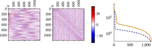
If we compare the singular values of the matrix ${\mathbf{A}}_h$ in Figure 4 (right) with those of the two datasets in Figure 3, we observe that the dominant singular values of the least square matrix computed with the CleanDataSET are the first thirty (similar to what happens in the singular values of the CleanDataSET itself in Figure 3), while those that are most relevant for the matrix constructed with the NoisyDataSET are the first one hundred. While this information is only qualitative, it does show that a non-negligible part of the local inverse problem can be approximated relatively well by the linear operator $F_h\left(\mathbf{u}\right)={\mathbf{A}}_h\mathbf{u}$, with an intrinsic dimension of around one hundred, when including noise, and much smaller when considering a clean dataset.

The statistical distribution of the test error in the CleanDataSET (i.e. the error defined in (15(15) $\mathrm{TE}\left(\right\{{\mathbf{u}}_j,{\mathbf{C}}_j{\}}_{j=1}^{N_{\mathrm{test}}}):=\frac{1}{N_{\mathrm{test}}}\sum _{j=1}^{N_{\mathrm{test}}}\Vert F_h\left({\mathbf{u}}_j\right)-{\mathbf{C}}_j{\Vert }_{{\ell }^{\mathrm{\infty }}}.$(15) ) for the CleanTestDataSET) is reported in Table 2 and depicted in the left panel of Figure 5. It shows an error which is, on average (orange dashed line), around $9\mathrm{\%}$. Even though such a model presents a relatively high error, we observe that it is still capable of capturing the overall qualitative behaviour of the doping profiles (see Figure 6).

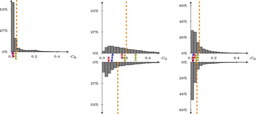
Figure 5. Statistical distribution of the errors on the predictions of our least square model, trained/tested on CleanTrainingDataSET/CleanTestDataSET (left), CleanTrainingDataSET/NoisySmallTestDataSET (center), and NoisyTrainingDataSET/NoisyTestDataSET. The bottom histograms are obtained by removing the average value of the doping. The dashed lines represent the average value of the error, while the arrows point to the 25, 50, and 75-percentile of the error on the top histogram, and show how these change when removing the average in the bottom histogram.

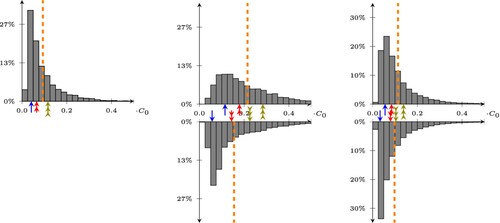
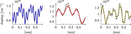
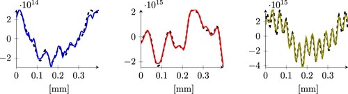
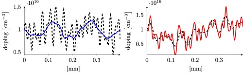
Figure 6. Three examples of predictions obtained using the least squares model applied to the CleanDataSET. The dashed grey line is the expected result, the continuous coloured lines are our predictions. The three plots represent samples whose error is close to the 25, 50 and 75-percentile (from left to right), and corresponds to the three arrows in the left histogram in Figure 5 of the same colour.

Next, we check how robust our two models are with respect to noise. As a first test, we use the linear operator generated from the CleanTrainingDataSET to predict the doping of the samples in the NoisyTestDataSET. Since this model has not been trained with data affected by noise, we observe a significant deterioration in the quality of the predictions, shown in the middle plot of Figure 5, where the average error is now around $20\mathrm{\%}$.

We believe that the main reason why the error increases so much is the fact that the noise introduces a shift in the average of the doping function that can not be physically estimated by our setup. In other words, Equation  (16(16) $C(\mathbf{x}=(x,y,z{)}^T;\text{β}=(C_0,\mathit{\alpha },\mathit{\lambda }{)}^T)=C_0(1+\sum _{i=1}^{N_b}{\alpha }_{i}n\frac{2\mathrm{\pi x}}{{\lambda }_i}),$(16) ) defines the admissible doping profiles with an average of (roughly) equal to $1\cdot {10}^{16}=C_0$ on the overall domain. When we introduce noise, this assumption does not hold anymore and we have no way to predict whether the average of the doping is the one we expect in the entire crystal sample. This is also coherent with the qualitative analysis in Equation  (17(17) $u_P(\mathbf{x},C)m-{\mathbf{e}}_x\cdot \mathrm{\nabla C}\left(\mathbf{x}\right).$(17) ), where we show that the value of the current is mostly related to the local variation of the doping and not to its average value.

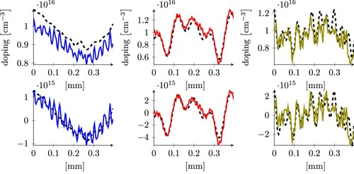
Removing the average from both the output of the model, and from the reference doping during testing leads to the results in the right plot of Figure 5 (bottom), where the error drops from $20\mathrm{\%}$ to $15\mathrm{\%}$. Indeed, we expect still a larger error w.r.t. to the histogram presented in Figure 5, since the test dataset includes noisy data which are not included in the training dataset. A few examples of predictions of the doping profile on ${\mathrm{\Sigma }}_h$ with noisy input data are shown in Figure 7.

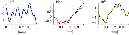
Figure 7. Three examples of predictions on the NoisyTestDataSet, using the least square model trained on the CleanTrainingDataSet, taken from the 25, 50, and 75 percentile of the error (from left to right), without removing the average of the doping (top), and removing the average (bottom). The samples in the plots have an error that corresponds to the arrows in the histograms in the middle of Figure 5 (including the colour).

An improvement of the error for the least square problem can be obtained by performing the training on the NoisyTrainingDataSET. The histogram of the error on the NoisyTestDataSET is shown in the right plot of Figure 5, where the error is now around $10\mathrm{\%}$ (see Table 2 for the details). It becomes apparent that training with noisy doping profiles also significantly reduces the need to remove the average doping value.

In summary, the least square model is able to predict doping profiles with an average error of around $10\mathrm{\%}$ for clean test data or noisy but properly average adjusted test data. However, it is possible to further improve the results by introducing nonlinearities in our models, for example using neural networks. We focus on multilayer perceptrons and residual neural networks in the following sections.

4.5. Multilayer perceptron

While the least square approach is a good starting point, its efficiency is only good if the inverse operator is close to a linear operator. For inverse problems associated to the van Roosbroeck system, this is not necessarily the case, and one may choose to introduce some nonlinearities in the approximation of $F_h$. Multilayer perceptrons [37] are among the most widely used feedforward neural networks, and they are the first natural candidate for general nonlinear function approximations. We consider networks consisting of a down-sampler ($L_1$), a multilayer perceptron with six layers ($L_2\dots L_7$), and an up-sampler ($L_8$). The main motivation for introducing the down-sampler and the up-sample layers is to avoid introducing “too many values” inside our model. Indeed, if we used directly the data from our datasets, then the first layer of our MLP should have 1200 neurons (which is the value of n defined in Section 4.2), which is a large number that would increase the complexity of the model and our probability of overfitting during the training. On the other hand, the signal is just a spatial function defined on Σ and we can interpolate the signal on a coarser grid obtaining a still accurate description of the signal while reducing the dimension of the space of the admissible inputs. The down-sampler layer we introduced uses cubic interpolation to describe the original signal on a coarse grid of evenly spaced points. The up-sampler, instead, performs cubic interpolation from the coarse grid to the original one we used for measuring the doping. In this way, we can compare results from different models in the same space, independently from the grid used by the MLP.

There is no a priori method to choose a suitable number of points for the coarse grid nor there exists a standard algorithm to select the number of neurons of each layer. Our strategy is to choose some reasonable values for each free hyperparameter of the model and then combine all the admissible choices to generate a set of candidate models. Unfortunately, we do not dispose of enough computational power to train all these models and, therefore, we need an algorithm to explore this set and to find a good choice for the hyperparameters.

First of all, let us describe the space of the admissible configurations. The number of points of the coarse grid (which coincides with the number of neurons of the input layer of the MLP) is chosen from the set $\{100+i50:i=0,\dots ,8\}$. The number of neurons of the MLP output layer $L_7$, which in principle can be different from the previous one, is chosen from the same set.

Let $\mathrm{\#}\left(L_i\right)$ denote the number of neurons in $L_i$. For each hidden layer $L_i$ of the MLP with $i=3,\dots ,6$, we randomly choose $\mathrm{\#}\left(L_i\right)$ in the set $\left\{\mathrm{\#}\right(L_{i-1}),\mathrm{\#}(L_{i-1})\pm 50,\mathrm{\#}(L_{i-1})\pm 100,\mathrm{\#}(L_{i-1})-200\}$ with the constraint that $\mathrm{\#}\left(L_i\right)>0$. In total, there are 71, 118 admissible configurations. There are fewer than $6^4\cdot 9^2$ configurations because some of them would lead to a negative amount of neurons. The multilayer perceptrons are implemented in PyTorch [38].

For a given configuration of the neural network, we apply the stochastic gradient descent (SGD) algorithm (without momentum and weight decay) to find the MLP that minimizes the mean square error loss defined in Equation  (14(14) $\mathrm{MSE}\left(\right\{{\mathbf{u}}_j,{\mathbf{C}}_j{\}}_{j=1}^{N_{\mathrm{train}}}):=\frac{1}{N_{\mathrm{train}}}\sum _{j=1}^{N_{\mathrm{train}}}\Vert F_h\left({\mathbf{u}}_j\right)-{\mathbf{C}}_j{\Vert }_{{\ell }^2}^2,$(14) ). For each network configuration, we fix the learning rate to a value that is chosen randomly in the interval $[{10}^{-3},1]$ and the batch size to 64. The number of training epochs is set to 1, 000.

We randomly select 10, 000 configurations where we vary both the structure of the MLP (choosing one of the 71,118 possible MLPs) as well as the learning parameters of SGD. To reduce the computational cost associated with the training of all the resulting neural networks, we apply the Asynchronous Successive Halving algorithm (ASHA) [39], a multi-armed bandit algorithm that has been optimized to run on a massive amount of parallel machines. The ASHA algorithm discards the worst $50\mathrm{\%}$ performers of the neural network population at each check point and proceeds with the training only for the most promising neural networks. Our implementation is based on the Ray library [40], which also takes care of distributing the jobs and coordinating the execution among different nodes during the computation.

The multilayer perceptron with the smallest ${\ell }^{\mathrm{\infty }}$ testing error defined in Equation  (15(15) $\mathrm{TE}\left(\right\{{\mathbf{u}}_j,{\mathbf{C}}_j{\}}_{j=1}^{N_{\mathrm{test}}}):=\frac{1}{N_{\mathrm{test}}}\sum _{j=1}^{N_{\mathrm{test}}}\Vert F_h\left({\mathbf{u}}_j\right)-{\mathbf{C}}_j{\Vert }_{{\ell }^{\mathrm{\infty }}}.$(15) ) (trained with CleanDataSET and tested with CleanTestDataSET), has six layers with 250, 250, 150, 100, 1000, 350 nodes, a batch size of 64, and a learning rate of 0.06. The statistical distribution of the error is reported in the middle part of Table 2, and depicted in the left plot of Figure 8. The ${\ell }^{\mathrm{\infty }}$ error is, on average, around $4.67\mathrm{\%}$. Even with such a simple neural network, we reduce the average error with respect to the least square model by of a factor two. Also, we obtain a much better statistical distribution, clearly shown in Figure 8.

Figure 8. Statistical distribution of the ${\ell }^{\mathrm{\infty }}$ errors on the predictions of our best multilayer perceptron, trained/tested on CleanTrainingDataSET/CleanValidationDataSET (left picture), CleanTrainingDataSET/NoisySmallTestDataSET (center), and NoisyTrainingDataSET/NoisyTestDataSET (right). The bottom histograms are obtained by removing the average value of the doping. The dashed lines represent the average value of the error, while the arrows point to the 25, 50, and 75-percentile of the error on the top histogram, and show how these transform when removing the average in the bottom histogram.

Furthermore, the resulting MLP is robust to noise, provided that we properly filter the average of the doping profile. A comparison between the statistical distribution of the errors (both with and without average) as well as the corresponding statistical distributions are shown in Table 2 and in Figure 8 (center). Testing with the NoisyTestDataSET while the MLP was trained with CleanDataSET shows (as expected) a large increase in the average error.

More robust results with respect to noise can be obtained by training again the best MLP on the full NoisyTrainingDataSET. We do not perform an additional hyperparameter tuning, but simply repeat the training stage on the same MLP. In this case, the larger dataset and the presence of noise induce an error when tested with the NoisyTestDataSET of around $5.92\mathrm{\%}$. This error can, again, be improved by removing the average as we did before, leading to a final error which is very close to the clean case ($4.96\mathrm{\%}$ vs $4.67\mathrm{\%}$). We show three doping reconstructions for this case in the 25, 50, and 75 percentile in Figure 9.

Figure 9. Three examples of predictions on the NoisyTestDataSet, with the best MLP model trained on the NoisyTrainingDataSet, taken from the 25, 50, and 75 percentile of the error, removing the average. The errors of the plots correspond to the arrows in the lower histogram in the right of Figure 8.

In summary, introducing a nonlinear MLP model has reduced the error roughly by a factor of two compared to the linear least square model. The average MLP is just below $5\mathrm{\%}$ for clean test data or noisy but properly average adjusted test data.

4.6. Residual neural network (ResNet)

In 2015, Kaiming et al. [41] introduced ResNets, feedforward convolutional neural network models, which, since then, have been widely used to solve different kinds of problems. One of the biggest advantages of ResNets (or, generally, of convolutional neural networks) over the multilayer perceptrons is their ability to learn 2D images. Interpreting the doping profiles in 2D probing region as an image, this is precisely what we need to achieve, too. Moreover, the proportionality shown in Equation (18(18) $u_P(x,C)m(f\ast ({\mathbf{e}}_x\cdot \mathrm{\nabla C}\left)\right)\left(x\right)=\frac{\mathrm{d}}{\mathrm{d}x}(f\ast C)\left(x\right).$(18) ), valid under additional assumptions, suggests that the photovoltage signal and the doping profile may be related by convolutions. Even assuming now a nonlinear relationship described via ResNets, we may still wish to exploit a convolutive structure to encompass the relationship in Equation  (18(18) $u_P(x,C)m(f\ast ({\mathbf{e}}_x\cdot \mathrm{\nabla C}\left)\right)\left(x\right)=\frac{\mathrm{d}}{\mathrm{d}x}(f\ast C)\left(x\right).$(18) ). Our reference implementation for residual neural networks (ResNet) is described in Ref. [41], with some important differences regarding the structure of the network.

First, in our LPS setup from Section 4.2, we consider one-dimensional data vectors $\mathbf{C}$ and $\mathbf{u}$ instead of two-dimensional images. The dimension is particularly relevant to choose the size of the network: In ResNets, the downsampling blocks reduce by a factor of two the size of the input, by first halving the size of the input in each direction (reducing the spatial indices by a factor four) and then doubling the number of channels. In our setup, this dimension reduction associated to the downsampling block does not happen because in the first step we only have one dimension to divide by two, and we end up with the same number of neurons after doubling the numbers of channels. Moreover, while the ImageNet database used to train the network described in Ref. [41] contains about one million images, our datasets are significantly smaller. We expect to face some overfitting and therefore we aim for a model with fewer parameters than the one described in Ref. [41]. Finally, we solve a regression problem instead of a classification one. The major consequences for our model are that we cannot use drop-out layers to reduce overfitting, and it is unclear if there is any benefit in using batch normalization layers. We keep the batch normalization layers because we expect the statistical distribution of our batches to be similar to each other, and the statistical distribution of the error for a simpler network (the MLP) shows an improvement in the performance of the model with noise when removing the average, suggesting that batch normalization layers are at least not harmful.

We build several ResNet models using PyTorch [38] and develop a strategy to find the best ones by adapting the model described in Ref. [41], and using the insight obtained from the MLP model presented in Section 4.5. Our best multilayer perceptron had 160,950 parameters that had to be optimized. We try to keep the number of parameters of our ResNet around the same order of magnitude. Of course, this means that we need to drastically simplify the model developed in Ref. [41], to find a model whose number of parameters is compatible with the size of our CleanTrainingDataSET.

Since training a ResNet is significantly more expensive compared to training a multilayer perceptron, we use a two-step strategy to reduce the computational cost of the hyperparameter tuning. The possible configurations of the ResNet that we allow in our models are detailed in Appendix 2 and correspond to a total of 48 configurations for the gate, 9 configurations for the encoder, and 18 configurations for the decoder, for a total of $7776$ possible configurations (Figure 10).

Figure 10. ${\ell }^{\mathrm{\infty }}$ errors of our model with respect to the parameters of the optimizer. In the top plot, the colours correspond to the networks RN1-RN4, as seen in Table 1. The other two plots (bottom row) are batch size and weight decay density plots computed via KernelDensity of sklearn.neighbours with a Gaussian kernel and a bandwidth of 0.02. Darker line colours correspond to bigger parameter values (batch size or weight decay).

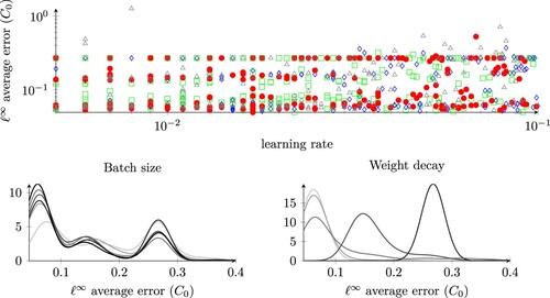
In the first step of our hyperparameter tuning, we restrict the parameters for the SGD optimizer to a fixed float number chosen in the interval $[5\times {10}^{-3},1\times {10}^{-1}]$ for the learning rate, and choose a batch size in the set $\{64,128,256,384,512\}$. We fix also the gradient clipping to 1 and the weight decay to 0. During this step, we randomly sampled 300 ResNet configurations among the 7776 generated according to Appendix 2, and for each one of them, we performed six trainings using different set of parameters for the SGD optimizer. Again, we rely on the ASHA algorithm as we did in Section 4.5. We compare the performances of the models after 5000 epochs of the SGD algorithm, and retain only four of the candidate ResNet models selected by the ASHA algorithm, which are described in Table 1.

In the second stage of the hyperparameter tuning, we keep the four structures of the ResNet models fixed, and enlarge the search space in the optimization parameters by defining a new set of admissible parameters: we choose the learning rate in the interval $[{10}^{-3},{10}^{-1}]$, the batch size in the set $\{32,64,128,256,384,512\}$, the gradient clipping in $\{{10}^{-2},{10}^{-1},1\}$, and we introduce some weight decay, with decay parameters chosen in the set $\{{10}^{-4},{10}^{-3},{10}^{-2},{10}^{-1},1\}$.

For each one of the four models, we perform 200 different trainings applying different parameters of the SGD optimizer, and finally select a winner, corresponding to RN3 in Table 1.

Table 1. The four ResNet models (RN1–RN4) identified in the first stage of the hyperparameter tuning by the ASHA algorithm.

	RN1	RN2	RN3	RN4
N. of channels	24	16	24	16
Gate conv. kernel size	9	5	7	3
Gate conv. stride	4	4	4	4
N. of encoder blocks	3	3	3	3
Block type:	FixedChannel	Basic	FixedChannel	FixedChannel
Downsampling:	True	True	True	True
Size of decoder layers	(100, 200)	(150, 150)	(200, 200)	(250, 200)
N. of parameters	102,188	324,048	141,440	138,994

Note: RN3 is the one selected in the second stage.

In Figure 11 we present the statistical distribution of the error for ResNet RN3 selected with the strategy outlined above. We observe that the average error we obtain using the CleanDataSET for both training and testing is around $5.47\mathrm{\%}$ (see Table 2 for the details). This number is slightly worse compared to the MLP case introduced in Section 4.5. In particular, we observe that the ResNet RN3 trained with the CleanDataSET is more sensitive to noise (see Figure 11, center figure) when compared to the MLP ($29.7\mathrm{\%}$ vs $21.2\mathrm{\%}$). This difference decreases when removing the average, but for the ResNet remains surprisingly worse than the least square model ($16\mathrm{\%}$ vs $15.5\mathrm{\%}$).

Figure 11. Statistical distribution of the errors on the predictions of our best ResNet, trained/tested on CleanTrainingDataSET/CleanTestDataSET (left), CleanTrainingDataSET/NoisySmallTestDataSET (center), and NoisyTrainingDataSET/NoisyTestDataSET (right). The bottom histograms are obtained by removing the average value of the doping. The dashed lines represent the average value of the error, while the arrows point to the 25, 50, and 75-percentile of the error on the top histogram, and show how these transform when removing the average in the bottom histogram.

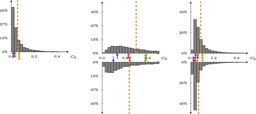
Table 2. Absolute errors w.r.t $C_0=1.0\times {10}^{16}{\mathrm{cm}}^{-3}$ corresponding to the coloured arrows as well as dashed lines showing in Figures 5,8, and 11 (from top to bottom).

Absolute error ($\times C_0$)		Average	25-th percentile	Median	75-th percentile
LS	C.C.	$9.32\mathrm{\%}$	$4.15\mathrm{\%}$	$6.53\mathrm{\%}$	$1.16\mathrm{\%}$
	C.N. w/ mean	$21.5\mathrm{\%}$	$11.5\mathrm{\%}$	$17.9\mathrm{\%}$	$28.4\mathrm{\%}$
	C.N. w/o mean	$15.5\mathrm{\%}$	$6.75\mathrm{\%}$	$10.5\mathrm{\%}$	$21.0\mathrm{\%}$
	N.N. w/ mean	$11.4\mathrm{\%}$	$5.72\mathrm{\%}$	$8.46\mathrm{\%}$	$13.8\mathrm{\%}$
	N.N. w/o mean	$9.81\mathrm{\%}$	$4.20\mathrm{\%}$	$6.47\mathrm{\%}$	$11.9\mathrm{\%}$
MLP	C.C.	$4.67\mathrm{\%}$	$1.03\mathrm{\%}$	$1.83\mathrm{\%}$	$3.98\mathrm{\%}$
	C.N. w/ mean	$21.2\mathrm{\%}$	$91.1\mathrm{\%}$	$17.3\mathrm{\%}$	$29.3\mathrm{\%}$
	C.N. w/o mean	$13.7\mathrm{\%}$	$4.15\mathrm{\%}$	$8.89\mathrm{\%}$	$19.7\mathrm{\%}$
	N.N. w/ mean	$5.92\mathrm{\%}$	$2.14\mathrm{\%}$	$3.60\mathrm{\%}$	$6.20\mathrm{\%}$
	N.N. w/o mean	$4.96\mathrm{\%}$	$1.44\mathrm{\%}$	$2.49\mathrm{\%}$	$4.67\mathrm{\%}$
ResNet	C.C.	$5.47\mathrm{\%}$	$1.60\mathrm{\%}$	$3.00\mathrm{\%}$	$6.80\mathrm{\%}$
	C.N. w/ mean	$29.7\mathrm{\%}$	$13.2\mathrm{\%}$	$22.3\mathrm{\%}$	$38.5\mathrm{\%}$
	C.N. w/o mean	$16.0\mathrm{\%}$	$5.27\mathrm{\%}$	$10.4\mathrm{\%}$	$21.2\mathrm{\%}$
	N.N. w/ mean	$8.67\mathrm{\%}$	$4.22\mathrm{\%}$	$6.20\mathrm{\%}$	$10.1\mathrm{\%}$
	N.N. w/o mean	$6.72\mathrm{\%}$	$3.15\mathrm{\%}$	$4.44\mathrm{\%}$	$7.06\mathrm{\%}$

Note: Here the second column categorized the training and testing datasets mentioned in the captions of the histogram figures. For instance, the row for “C.N. w/ mean” in the block of MLP shows the errors in the top-mid histogram in Figure 8 which is trained/tested on CleanTraining DataSET/NoisySmallTestDataSET.

When we keep the structure of RN3, and train the network on the NoisyTrainingDataSET, we obtain the results shown in Figure 11 on the right. An example of reconstruction obtained with RN3 with a sample from the NoisyTestDataSET is shown in Figure 12. In this case the average error on the NoisyTestDataSET is around $6.72\mathrm{\%}$, which is slightly worse than the result obtained with the MLP network.

Figure 12. Three examples of predictions on the NoisyValidationDataSet, with the best ResNet RN3 model trained on the NoisyTrainingDataSet, taken from the 25, 50, and 75 percentile of the error, removing the average of the doping. The colours of the plots indicate the arrows in the right bottom histogram in Figure 11.

5. Summary and outlook

The aim of this paper was to properly model and numerically solve general ill-posed inverse photovoltage technologies where measured photovoltage signals are used to reconstruct local doping fluctuations in a semiconductor crystal. The underlying charge transport model is based on the van Roosbroeck system as well as Ohm's law. We presented three different data-driven approaches to solve a physically relevant local inverse problem, namely via least squares, multilayer perceptrons, and residual neural networks. The methods were trained on synthetic datasets (pairs of discrete doping profiles and corresponding photovoltage signals at different illumination positions) which are generated by efficient physics-preserving finite volume solutions of the forward problem. While the linear least square method yields an average absolute ${\ell }^{\mathrm{\infty }}$ error of $9.3\mathrm{\%}$, the nonlinear networks roughly halve this error to $4.7\mathrm{\%}$ and $5.5\mathrm{\%}$, respectively, after optimizing relevant hyperparameters. Our method turned out to be robust with respect to noise, provided that training is repeated with larger, noisy, datasets. In this case, the error is around $9.8\mathrm{\%}$, $5\mathrm{\%}$, and $6.7\mathrm{\%}$ respectively. Removing the average doping value from the data was more important to reduce the testing error for clean datasets than for noisy ones. The datasets, python codes, and resulting trained networks are available in the repository [36].

Future research may go into different directions: the numerical simulation served as a proof of principle and was limited to a 2D version of the photovoltage problem. For the 3D problem, efficient data generation strategies need to be designed. Furthermore, it is clear that different doping profiles may correspond to similar signals. On the one hand, this is intrinsically dependent on the technology that we apply to recover the signal: we hit the crystal with a laser that has a finite laser spot radius (in our case, around $20\mu$ m), and we cannot expect to resolve oscillations with smaller wave lengths. On the other hand, our models do not have a way to distinguish between two doping profiles that deliver the same signal but are exposed, during training, to many such cases. In Figure 13, for example, we show two examples of doping profiles that have errors on the far right regions of the histograms in Figures 8 and 11. The figure shows how in some cases, the inverse problem is oblivious to higher oscillations, and both neural network types will have cases in which they return an answer which is either too smooth w.r.t. the expected result, (left panel of Figure 13) or too oscillatory (right panel of Figure 13).

Figure 13. An example of an outliers using the MLP model (left) and the ResNet model RN3 (right). The dashed line represents the expected doping profile sample, and the continuous line is the output of the neural networks.

A possible focus of future research could be to study how to resolve this ambiguity, which is intrinsic to the ill-posedness of the discrete local photovoltage inverse problem. Finally, we aim to extend our data-driven approach to opto-accoustic imaging, replacing the charge transport model with appropriate thermal expansion models.

Disclosure statement

No potential conflict of interest was reported by the author(s).

Appendices

Appendix 1. Generation of noise

In order to introduce noise in the doping profile (16(16) $C(\mathbf{x}=(x,y,z{)}^T;\text{β}=(C_0,\mathit{\alpha },\mathit{\lambda }{)}^T)=C_0(1+\sum _{i=1}^{N_b}{\alpha }_{i}n\frac{2\mathrm{\pi x}}{{\lambda }_i}),$(16) ), we perturb both the doping amplitudes as well as the wavelength. To perturb the doping amplitudes, we start from some elements of ${\mathcal{C}}_{\mathrm{TF}}$. We introduce imperfections of the doping profile that may be interpreted physically with a slight perturbation during the growth process (for example, due to a fluctuation of the temperature), we choose a random function $f_n\left(x\right)$ and define a perturbed doping of the form $\tilde{C}\left(x\right):=C\left(x\right)+f_n\left(x\right)$. We require that $f_n\left(x\right)\ll C\left(x\right)$ for any x. To generate $f_n\left(x\right)$, we pick 129 equally-spaced points $x_i$ across the silicon sample and randomly sample 129 values from a normal distribution (with 0 mean and standard deviation equal to 1), obtaining a family of values $s_i$. Denoting the maximal variation of C with ${\mathrm{\Delta }}_C:=\underset{x\in [-\ell /2,\ell /2]}{max}C\left(x\right)-\underset{x\in [-\ell /2,\ell /2]}{min}C\left(x\right)\mathrm{we}\mathrm{define}{f}_n\left(x_i\right):=k{s}_i{\mathrm{\Delta }}_C,$for $0<k\ll 1$. For any other point $x\ne x_i$ across the sample, we compute $f_n\left(x\right)$ by cubic spline interpolation. Next, we perturb the wavelengths. In (16(16) $C(\mathbf{x}=(x,y,z{)}^T;\text{β}=(C_0,\mathit{\alpha },\mathit{\lambda }{)}^T)=C_0(1+\sum _{i=1}^{N_b}{\alpha }_{i}n\frac{2\mathrm{\pi x}}{{\lambda }_i}),$(16) ), we assumed that the doping has fluctuations with constant wavelength across the entire domain. We weaken this assumption by introducing a non-periodic perturbation in the argument of the sinusoidal functions: we consider a differentiable function $t:[-\ell /2,\ell /2]⟶[-\ell /2,\ell /2]$, such that $t(-\ell /2)=-\ell /2$, $t\left(\ell /2\right)=\ell /2$, and $t^{\prime }\left(x\right)>0$ for every x; then we define the perturbed doping as $\overline{C}\left(x\right):=\tilde{C}\left(t\right(x\left)\right)$.

In order to generate t, we impose that $p\left(x\right):=t\left(x\right)-x$ is a polynomial of degree 2 or 3. Due to the properties of the function t, we obtain that $p(-\ell /2)=0$ and $p\left(\ell /2\right)=0$. We randomly decide whether to use a polynomial of degree 2 or of degree 3, that is, we use $p\left(x\right)=k(x+\ell /2)(x-\ell /2)\mathrm{or}p\left(x\right)=k(x+\ell /2)(x-\ell /2)(x-\alpha )$where k and α are random constants chosen so that $p^{\prime }\left(x\right)>-1$ for every x.

Applying the transformation on a doping function, we can generate new samples for our dataset whose doping can not be described simply by choosing some suitable parameters in (16(16) $C(\mathbf{x}=(x,y,z{)}^T;\text{β}=(C_0,\mathit{\alpha },\mathit{\lambda }{)}^T)=C_0(1+\sum _{i=1}^{N_b}{\alpha }_{i}n\frac{2\mathrm{\pi x}}{{\lambda }_i}),$(16) ).

Appendix 2. ResNet structure

Exactly as we did for the MLP models, all of our ResNets are preceded by a down-scaling interpolation layer and, at the end, there is an up-scaling layer that restores the original dimension of the data; the scaling layers use cubic interpolation to describe the signals or the dopings on different spacial grids. In this case, we fix the size of the coarse grid to 256, i.e. to a power of two that is close to the size that we have seen performs better in the MLP model. Using a power of two we ensure that the downscaling blocks of the ResNet always deal with an even number of neurons.

Following [41], the structure of our ResNets is made of three different parts: the gate, which elaborates the input from the down-scaling layer; the encoder, which applies the convolutional layers in order to extract the most relevant features of the signal; and the decoder, which takes as input the features recognized by the encoder and produces the model prediction. In the following part, we describe in detail the structure of each part of the network and its associated hyperparameters.

Gate This is the first part of our network (after the down-sampling layer). It consists of a convolutional layer, a batch normalization layer, and an activation layer. In the convolutional layer, we choose the kernel sizes from the set $\{3,5,7,9\}$. The number of output channels, instead, is chosen from the set $\{8,16,24,32\}$. Finally, the stride of the convolution layer is chosen from the set $\{1,2,4\}$. This leads to $4\times 4\times 3=48$ possible convolutional layers for our gate. Taking into account that the activation layer always applies a ReLU (that does not require parameters) and that also the normalization layer is fixed, we have a total of 54 possible configurations for the gate.

Encoder The encoder is built by stacking several blocks of the same type. We consider two different kinds of blocks: the “basic blocks” described in Ref. [41] and the “fixed channel block”. Both blocks are made of the following layers: a convolutional layer, a batch normalization, a ReLU activation layer, another convolution, and, finally, a normalization. The two convolutional layers have a fixed kernel size of 3: they do not have bias and the padding is chosen so that the size of the output is preserved (therefore, in our case, the padding is equal to 1).

The difference between a ResNet and a plain convolutional neural network is the fact that the input of each block is not simply the output of the previous one. Instead, each block $B_i$ saves the input $x_i$ it receives and, after its computations, sums its output $B_i\left(x_i\right)$ with the original input $x_i$ (or with a simple function of the input $s_i\left(x_i\right)$). In this way, the input of the layer $B_{i+1}$ is (A1) $x_{i+1}=x_i+B_i\left(x_i\right).$(A1) Usually, in a ResNet, the shape of the data may change along the layers; indeed, $x_i$ is a bidimensional tensor: the first index represents the spatial position and while the second one is the channel. The input of the first block of the encoder has shape (256, $k_1$) where $k_1$ is the number of output channels of the gate but, while the blocks become deeper, $k_i$ increases and the number of points decreases. A block $B_i$ so that $B\left(x_i\right)$ has a different shape respect to $x_i$ is called a downsampler block. In our networks, each downsampler block halves the size of the first index of the tensor; so, for example, the output of the first downsampler block will have size (128, $k_i$). The only difference between the “basic blocks” and the “fixed channel blocks” is in how the perform the downsample: a downsampling basic block increases the number of channels by a factor two, while a fixed channel block does not.

It is worth noting that Equation  (A1(A1) $x_{i+1}=x_i+B_i\left(x_i\right).$(A1) ) can not be applied by the downsampling blocks because of the different shapes of the tensors. In this case, the equation becomes $x_{i+1}=s_i\left(x_i\right)+B_i\left(x_i\right).$where $s_i$ is called ”shortcut operation”; in our network, $s_i$ is performed by a convolutional layer with kernel size equal to 1 and stride equal to 2 (basic blocks), or kernel size equal to 2 and stride equal to 2 (for the fixed channel blocks), followed by a normalization block.

The convolutional layer of the shortcut of the fixed channel blocks forbids any communication between channels, i.e. each element of the output tensor depends only on the values of the elements of the input tensor that share the same index for the channel (or, in other words, using PyTorch we impose that the number of groups of the convolutional layer is equal to the number of channels). For what concerns the computation of the output (and not the shortcut), the dimensional reduction is obtained by setting the stride of the first convolutional layer to 2.

Therefore, the only free parameters that we have left for our encoder are the number of blocks, their kind, and a downsampling flag for each block. Our encoders consist of one, two, or three blocks of the same kind. For encoders made of basic blocks, we allow two different configurations of the downsample flag: true for all blocks or false for all blocks. For fixed channel blocks, we always set the downsample flag to true. We have a total of 6 configurations for the encoders with the basic blocks and 3 configurations that use the fixed channels blocks, for a total of 9 possible configurations.

Decoder This is essentially a multilayer perceptron, and we allow 1 or 2 hidden layers. If we choose a configuration with 1 layer, the size of this layer could be 100, 150 or 200. With 2 layers, there is a total of 15 possible configurations obtained by choosing the size of the first layer in $\{100,150,200,250,300\}$ and the second one in $\{100,150,200\}$. In total, we have therefore 18 different configurations for the decoder.

References

- Wittry DB, Kyser DF. Measurement of diffusion lengths in direct-gap semiconductors by electron-beam excitation. J Appl Phys. 1967;38:375–382. doi: 10.1063/1.1708984
- Bajaj J, Bubulac LO, Newman PR, et al. Spatial mapping of electrically active defects in HgCdTe using laser beam-induced current. J Vac Sci Technol A: Vac Surfaces Films. 1987;5(5):3186–3189. doi: 10.1116/1.574834
- Jastrzebski L, Lagowski J, Cullen GW, et al. Hydrogenation induced improvement in electronic properties of heteroepitaxial silicon-on-sapphire. Appl Phys Lett. 1982;40:713–716. doi: 10.1063/1.93201
- Lüdge A, Riemann H. Doping inhomogeneities in silicon crystals detected by the lateral photovoltage scanning (LPS) method. Inst Phys Conf Ser. 1997;160:145–148.
- Kayser S, Farrell P, Rotundo N. Detecting striations via the lateral photovoltage scanning method without screening effect. Opt Quant Electron. 2021;53:288. doi: 10.1007/s11082-021-02911-1
- Farrell P, Kayser S, Rotundo N. Modeling and simulation of the lateral photovoltage scanning method. Comput Math Appl. 2021;102:248–260. doi: 10.1016/j.camwa.2021.10.017
- Vogel CR. Computational methods for inverse problems. SIAM; 2002. https://epubs.siam.org/doi/book/10 .1137/1.9780898717570?mobileUi=0.
- Kaipio J, Somersalo E. Statistical and computational inverse problems. New York, NY: Springer; 2006.
- Leitao A, Markowich P, Zubelli J. On inverse doping profile problems for the stationary voltage-current map. Inverse Problems. 2006;22:1071–1088. doi: 10.1088/0266-5611/22/3/021
- Burger M, Engl HW, Leitao A, et al. On inverse problems for semiconductor equations. Milan J Math. 2004;72:273–313. doi: 10.1007/s00032-004-0025-6
- Peschka D, Rotundo N, Thomas M. Doping optimization for optoelectronic devices. Opt Quant Electron. 2018;50:125. doi: 10.1007/s11082-018-1393-4
- Farrell P, Rotundo N, Doan D, et al. Mathematical methods: drift-diffusion models. In: Piprek J, editor. Handbook of optoelectronic device modeling and simulation; ch. 50, Vol. 2. Boca Raton: CRC Press; 2017. p. 733–771. doi: 10.4324/9781315152318.
- Scharfetter D, Gummel H. Large-signal analysis of a silicon read diode oscillator. IEEE Trans Electron Devices. 1969;16:64–77. doi: 10.1109/T-ED.1969.16566
- Kayser S, Lüdge A, Böttcher K. Computational simulation of the lateral photovoltage scanning method. In: Proceedings of the 8th International Scientific Colloquium. Riga: IOP Publishing Ltd; 2018. p. 149–154.
- Kayser S. The lateral photovoltage scanning method to probe spatial inhomogeneities in semiconductors: a joined numerical & experimental investigation [dissertation]. Brandenburg University of Technology; 2021.
- Raissi M, Perdikaris P, Karniadakis GE. Physics-informed neural networks: a deep learning framework for solving forward and inverse problems involving nonlinear partial differential equations. J Comput Phys. 2019;378:686–707. doi: 10.1016/j.jcp.2018.10.045
- Ray D, Hesthaven JS. An artificial neural network as a troubled-cell indicator. J Comput Phys. 2018;367:166–191. doi: 10.1016/j.jcp.2018.04.029
- Mishra S. A machine learning framework for data driven acceleration of computations of differential equations. Math Eng. 2019;1:118–146. doi: 10.3934/Mine.2018.1.118
- Lye KO, Mishra S, Molinaro R. A multi-level procedure for enhancing accuracy of machine learning algorithms. Eur J Appl Math. 2021;32:436–469. doi: 10.1017/S0956792520000224
- Han J, Jentzen A, Weinan E. Solving high-dimensional partial differential equations using deep learning. Proc Natl Acad Sci. 2018;115:8505–8510. doi: 10.1073/pnas.1718942115
- Han J, Jentzen A. Deep learning-based numerical methods for high-dimensional parabolic partial differential equations and backward stochastic differential equations. Commun Math Stat. 2017;5:349–380. doi: 10.1007/s40304-017-0117-6
- Chen Y, Lu L, Karniadakis GE, et al. Physics-informed neural networks for inverse problems in nano-optics and metamaterials. Opt Express. 2020;28:11618–11633. doi: 10.1364/OE.384875
- Mishra S, Molinaro R. Estimates on the generalization error of physics-informed neural networks for approximating a class of inverse problems for PDEs. IMA J Numer Anal. 2022;42:981–1022. doi: 10.1093/imanum/drab032
- Lye KO, Mishra S, Ray D, et al. Iterative surrogate model optimization (ISMO): an active learning algorithm for PDE constrained optimization with deep neural networks. Comput Methods Appl Mech Eng. 2021;374:113575. doi: 10.1016/j.cma.2020.113575
- Nguyen HV, Bui-Thanh T. Model-constrained deep learning approaches for inverse problems. arXiv:2105.12033, 2021.
- Sheriffdeen S, Ragusa JC, Morel JE, et al. Accelerating PDE-constrained inverse solutions with deep learning and reduced order models. arXiv:1912.08864, 2019.
- Knapp E, Battaglia M, Stadelmann T, et al. Xgboost trained on synthetic data to extract material parameters of organic semiconductors. In: 2021 8th Swiss Conference on Data Science (SDS). Lucerne: IEEE; 2021. p. 46–51. doi: 10.1109/SDS51136.2021.00015
- Markowich PA. The stationary semiconductor device equations. Vienna: Springer; 1986.
- Selberherr S. Analysis and simulation of semiconductor devices. Wien, New York: Springer; 1984.
- Alì G, Rotundo N. An existence result for elliptic partial differential–algebraic equations arising in semiconductor modeling. Nonlinear Anal Theory Methods Appl. 2010;72(12):4666–4681. doi: 10.1016/j.na.2010.02.046
- Busenberg S, Fang W, Ito K. Modeling and analysis of laser-beam-induced current images in semiconductors. SIAM J Appl Math. 1993;53:187–204. doi: 10.1137/0153012
- Arridge S, Maass P, Öktem O, et al. Solving inverse problems using data-driven models. Acta Numer. 2019;28:1–174. doi: 10.1017/S0962492919000059
- Li H, Schwab J, Antholzer S, et al. NETT: solving inverse problems with deep neural networks. Inverse Problems. 2020;36:065005. doi: 10.1088/1361-6420/ab6d57
- Adler J, Öktem O. Solving ill-posed inverse problems using iterative deep neural networks. Inverse Probl. 2017;33(12):124007. doi: 10.1088/1361-6420/aa9581
- Kayser S, Rotundo N, Dropka N, et al. Assessing doping inhomogeneities in gaas crystal via simulations of lateral photovoltage scanning method. J Cryst Growth. 2021;571:126248. doi: 10.1016/j.jcrysgro.2021.126248
- Piani S, Lei W, Rotundo N, et al. Software repository for data-driven reconstruction of doping profiles in semiconductors. 2022. doi: 10.5281/zenodo.7294848
- Goodfellow I, Bengio Y, Courville A. Deep learning. Cambridge, MA: MIT press; 2016.
- Paszke A, Gross S, Massa F, et al. Pytorch: an imperative style, high-performance deep learning library. In: Wallach H, Larochelle H, Beygelzimer A, d'Alché-Buc F, Fox E, and Garnett R, editors. Advances in neural information processing systems; Vol. 32. New York: Curran Associates, Inc.; 2019. p. 8024–8035.
- Li L, Jamieson K, Rostamizadeh A, et al. A system for massively parallel hyperparameter tuning. arXiv, 2018.
- Moritz P, Nishihara R, Wang S, et al. Ray: a distributed framework for emerging AI applications. Proceedings of the 13th USENIX Symposium on Operating Systems Design and Implementation (OSDI ’18), Carlsbad, CA, USA; 2018, October 8–10. ISBN 978-1-939133-08-3.
- He K, Zhang X, Ren S, et al. Deep Residual Learning for Image Recognition. 2016 IEEE Conference on Computer Vision and Pattern Recognition (CVPR), Las Vegas, NV, USA; 2016. p. 770–778. doi: 10.1109/CVPR.2016.90