
 ?Mathematical formulae have been encoded as MathML and are displayed in this HTML version using MathJax in order to improve their display. Uncheck the box to turn MathJax off. This feature requires Javascript. Click on a formula to zoom.
Abstract
The novel coronavirus SARS-Cov-2 is a pandemic condition and poses a massive menace to health. The governments of different countries and their various prohibitory steps to restrict the virus's expanse have changed individuals' communication processes. Due to physical and financial factors, the population's density is more likely to interact and spread the virus. We establish a mathematical model to present the spread of the COVID-19 in worldwide. In this article, we propose a novel mathematical model (‘’) to assess the impact of using hospitalization, quarantine measures, and pathogen quantity in controlling the COVID-19 pandemic. We analyse the boundedness of the model's solution by employing the Laplace transform approach to solve the fractional Gronwall's inequality. To ensure the uniqueness and existence of the solution, we rely on the Picard-Lindelof theorem. The model's basic reproduction number, a crucial indicator of epidemic potential, is determined based on the greatest eigenvalue of the next-generation matrix. We then employ stability theory of fractional differential equations to qualitatively examine the model. Our findings reveal that both locally and globally, the endemic equilibrium and disease-free solutions demonstrate symptomatic stability. These results shed light on the effectiveness of the proposed interventions in managing and containing the COVID-19 outbreak.
1. Introduction
The Wuhan Health Commission in the province of China alerted the World Health Organization (WHO) of a group of 27 cases of pneumonia with an unknown etiological cause, which was regularly reported to the Wuhan city market around the end of December 2019. Chinese officials, On January 7, 2020, a new strain of the Corona virus family was identified as the source of the epidemic. The virus's medical observation was given the designation COVID-19. WHO declared a pandemic on the 12th of March, [Citation1–4]. Symptoms include sore throat, fever, dry cough, fatigue, and shortness of breath. In general, infections such as parasite infection by Cryptosporidia may occur without any symptoms.
The aim of the research was to construct a new ‘’ compartment model for predicting corona virus epidemiological dynamics. A model that presents the spreading dynamic of COVID-19 should be developed. In this case, Chen and Zhao [Citation5] established a ‘SUQC’ mathematical model to describe the transmission dynamics of coronavirus. Similarly, López et al. [Citation6] developed a new model of COVID-19, including healthy People, close contacts, and infected people.
Khajanchi et al. [Citation7] developed the COVID-19 model with quarantine for the transmission dynamics of COVID-19 and calibrated the model for the four provinces of India with daily and accumulated cases. Further, they have conducted a detailed theoretical analysis of the basic reproductive numbers and predicted accumulated cases. Moreover, the study suggested that quarantine, unreported and reported individuals as well as intervention policies like lock down, and face masks can play a significant role in controlling the spread of corona virus. Also, S. Choi and Moran. Ki [Citation8] developed a deterministic SEIHR mathematical model, in which they evaluated the effectiveness of control measures. Also, Lin et al. [Citation9] modelled the outbreak in China with governmental action and individual reaction (city lock down, holiday extension, quarantine, and hospitalization). Also Wang and Yang [Citation10] developed a model to investigate the corona virus disease outbreak.
Non-locality is the key areas of interest in the fractional calculus (FC) applications. There are fascinating phenomena called memory effects, this means that their conditions do not depend only on time and position even on the previous condition [Citation11]. Fractional differential equation (FDE) has numerous important in different fields of study including physics, biophysics, aerodynamics, electron-analytical chemistry, capacitor theory, biology, and electrical circuits [Citation12–20]. The Caputo derivative is one of the widely used definitions of fractional derivatives, and it differs from other fractional derivative definitions, such as the Riemann-Liouville derivative and the Grünwald-Letnikov derivative, in how it handles initial conditions and initial values.The Caputo derivative is most commonly used when we are dealing with fractional differential equations that involve initial conditions, as it leads to more physically meaningful solutions by considering the initial state of the system. The Riemann-Liouville derivative is used when initial values are involved in fractional differential equations. However, it can lead to solutions that are not physically meaningful in some cases, especially when dealing with real-world systems with initial conditions.The Grünwald-Letnikov derivative is commonly used in numerical methods for approximating fractional derivatives. It is straightforward to implement and provides accurate results when used with small values of h. However, it may not be suitable for all types of fractional differential equations, especially those involving initial conditions.
There have been several recent studies on epidemiological modelling using the FD equation [Citation21–26]. The most used fractional derivative by mathematicians is Rieman-Liouville fractional derivative, but this procedure is not worthy for most real world-problems. Therefore, an important definition was introduced by Caputo [Citation27]. Since the disease transmission rate is uncertain, we develop a mathematical model to present the spread of the COVID-19 in India and worldwide. This model is helpful for further modelling studies [Citation28–30], and we can compare our model with previous mathematical models with actual data values (MoHFW India) (Corona virus disease (COVID-19) 2020) for the authentication of the model. The paper is organised as follows: Section 2 is related to the mathematical model formulation and some basic definitions and theorems. In Sections 3 and 4, we study the boundedness and uniqueness of the solution of the model, respectively. Section 5 present the disease free and endemic equilibrium points. Section 6 describe the basic reproduction number of the model.Local and Global stability are presented in Sections 7 and 8, respectively. Some numerical simulations are executed to illustrate the analytical results in Section 9. Finally, conclusions are presented in Section 10.
2. Model formulation
A fractional ‘’ mathematical model of the COVD-19 was developed in this part. We consider the whole population
into seven classes: susceptible individuals
, latent individuals
, infected individuals
, quarantined individuals
, hospitalized individuals
, and the recovered individuals as
.
represents the quantity of pathogens present in the environment.
The COVID-19 transmission dynamics are represented in Figure flow chart.
Figure 1. Flow diagram of the COVID-19 Model (Equation1(1)
(1) ).
![Figure 1. Flow diagram of the COVID-19 Model (Equation1(1) {0cDtγ[S]=σ−βSN(I+θL)−υS−πSP,0cDtγ[L]=βSN(I+θL)−(υ+ϖ+τ)L+πSP,0cDtγ[I]=τL−(υ+δ+υi+φ+α+ϕ)I,0cDtγ[Iq]=ϕI−(υ+ϵ+υq)Iq,0cDtγ[Ih]=φI−(υ+λ+υh)Ih,0cDtγ[R]=δI+ϖL+λIh+ϵIq−υR,0cDtγ[P]=αI−υpP,(1) ).](/cms/asset/b8e4bd63-8111-4e2c-9fbc-0af197ba6a08/gipe_a_2326982_f0001_oc.jpg)
The virus can spread in two ways, according to scientists. Specifically, direct human-to-human and environmental-to-human transmission. Infected persons spread COVID-19 at a rate of π, according to the epidemic statistics, and are assigned to the latent individuals . When infected individuals sneeze or cough, the virus spreads to the surroundings they are in. Because pathogen
may survive in the environment for several days,
persons who are in close touch with it are likely to get infected. The rate of transmission from
to
due to contact with
is represented by π. Infected people with serious illnesses are admitted to hospitals at a rate of φ. In addition, individuals that were quarantined or hospitalised recovered from COVID-19 naturally at rates of ϵ and λ, respectively, and were placed in the recovered class
.
The Caputo derivative is used to develop a mathematical model is given by
(1)
(1)
with the following initial conditions
Detailed description of relevant parameters and state variables of the newly proposed COVID-19 model are well explained in Table .
The paper is arranged as: Section 1 gives the introduction. Section 2 includes model formulation and basic definitions. Boundedness and uniqueness for the solution are considered in Sections 3 and 4, respectively. Section 5 is devoted to the disease free equilibrium point (DFE) point. Basic reproduction is found in Section 6. The local and global stabilities are discussed in Sections 7 and 8, respectively. The numerical discussion is considered in Section 9. The last section is the conclusion of our work.
Table 1. Biological interpretations of parameters.
Definition 2.1
[Citation31]
Let be a smooth function, then the Caputo fractional derivative of
is
where,
.
Definition 2.2
[Citation32]
Let be a smooth function, then the fractional integral of order
for
is defined by
and
where
.
The following is an expression of a general n-dimension autonomous system:
(2)
(2)
Theorem 2.3
[Citation31]
For an equilibrium point for the system in Caputo sense (Equation2
(2)
(2) ) and
be the domain such that
and let
, be a continuously differentiable function. If
(3)
(3)
Then,
(4)
(4)
∀
and
, where
,
and
are positive definite continuous functions in Ξ, then the point
of (Equation2
(2)
(2) ) is stable asymptotically.
3. Boundedness of the system
The size of each population class varies over time in our suggested model (Equation1(1)
(1) ), and the overall population size
is provided by
Using the Caputo fractional derivative and the Caputo derivative linearity property, we get
(5)
(5)
We solve the Gronwall's inequality (Equation5
(5)
(5) ) using the Laplace transform with initial conditions
,
(6)
(6)
We obtain, when we split (Equation6
(6)
(6) ) into partial fractions.
(7)
(7)
By expanding through the Talyor series, we get
Therefore, (Equation7
(7)
(7) ) becomes
(8)
(8)
The inverse Laplace transform is applied to (Equation8
(8)
(8) )
(9)
(9)
Since
, or
. Therefore,
(10)
(10)
We are now utilising the Mittag–Leffler function definition
(11)
(11)
where,
and
are the series of entire function which converges for any argument, hence, the solution of Model (Equation1
(1)
(1) ) is bounded.
4. Uniqueness of the solution
Using fixed point theory, we discuss the uniqueness of the model's solution. Let us rewrite the proposed model (Equation1(1)
(1) ) in the following way.
(12)
(12)
where
(13)
(13)
We can write the model (Equation1
(1)
(1) ) as
(14)
(14)
where
Theorem 4.1
Lipschitz continuity is satisfied by System (Equation14(14)
(14) ).
Proof.
This implies
(15)
(15)
Hence, the function
is continuous and bounded.
The following theorem was constructed using the Picard–Lindelof theorem [Citation33].
Theorem 4.2
Let and
.
Let be a continuous and bounded function, that is ∃
such that
, since
satisfies Lipschitz continuity. If
, then there exist a unique
that satisfied the problem (Equation14
(14)
(14) ), where
.
Proof.
Let , clearly T is complete metric space because
and its closed set.
The following is an equivalent integral equation for the system (Equation14(14)
(14) ):
(16)
(16)
We define
in T as
(17)
(17)
We need to verify that (Equation17
(17)
(17) ) satisfies the contraction mapping principle hypothesis.
Firstly, we show that
(18)
(18)
Equivalently,
(19)
(19)
Clearly, the operator
maps T onto itself.
We need to demonstrate that T is a contraction.
Thus
(20)
(20)
According to hypothesis
, T is contraction and has a single fixed point. Hence, system (Equation14
(14)
(14) ) has unique solution.
5. Disease free and endemic equilibrium points
We set the right-hand sides of all equations in (Equation1(1)
(1) ) to zero to determine
of the system (Equation1
(1)
(1) ).
(21)
(21)
Let
, which means that
and
too. Hence we have
(22)
(22)
Therefore,
of the considered model (Equation1
(1)
(1) ) is given by
, which is always feasible.
To find the model endemic equilibrium point (Equation1(1)
(1) ), where at least one disease class is not zero. The steps below must be followed. Let
be the endemic equilibrium point of the model (Equation1
(1)
(1) ) and is given by
(23)
(23)
where,
6. Basic reproduction number 
In this section, we use the next generation matrix approach to compute the basic reproduction number ().
Let the matrices for transition and new infections terms of the model (Equation1(1)
(1) ) be V and F, respectively. Let
then;
The Jacobian matrix of
and
calculated at the disease free equilibrium (
are
Let,
and
.
Now,
Therefore, the next generation matrix of model (Equation1
(1)
(1) ) is
and the characteristic equation of
is given by
where,
. Eigenvalues of the above characteristic equation are
Therefore, the largest eigenvalue of
is
Thus,
of the considered model is
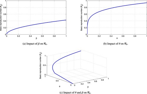
Figure represents the dynamics of with respect to the transmission rates β and θ.
7. Local stability
From system (Equation1(1)
(1) ), we construct the following matrix
where
Figure 2. Dynamics of with respect to transmission rates β and θ. (a) Impact of β on
. (b) Impact of θ on
and (c) Impact of θ and β on
.
Theorem 7.1
When , the disease free equilibrium
is locally asymptotically stable.
Proof.
The Jacobian matrix of the considered model at is given by
We get the eigenvalues
with
where,
. The imaginary portion of all eigenvalues is obviously zero. Therefore,
Hence,
is LAS.
Theorem 7.2
If , endemic equilibrium Point
is locally asymptotically stable.
Proof.
can be describe as
(24)
(24)
After the Linearizing around
we obtain
where
Characteristic equation of the above Jacobian matrix
(25)
(25)
where
The stability criterion is defined by Rouh-Hurtwiz as follows: the equation's equilibrium point is stable if these inequalities are satisfied
To begin, use
. Now,
, we can do this if
then
. For
, it is also clear, if
then
.
Now, for , if
then
.
Lastly, ,
then
.
The Routh–Hurwitz stability criteria are satisfied if because all of the conditions are dependent on
. Hence,the endemic equilibrium is asymptomatically stable when
.
8. Global stability
Theorem 8.1
When , the disease free equilibrium point
is globally asymptomatically stable.
Proof.
To derive the Lyapunov candidate function for fractional order as in [Citation16], consider the family of quadratic Lyapunov function
where
. We defined the Lyapunov function as
(26)
(26)
Using the linearity property of the Caputo operator:
(27)
(27)
Using Lemma 2 [Citation15], we get
(28)
(28)
Thus
(29)
(29)
Substituting the point
into (Equation29
(29)
(29) ), we get
Therefore
(30)
(30)
where
Thus,
. The equilibrium point
is thus globally asymptotically stable, according to Theorem 2.3.
Theorem 8.2
When , the point
is globally asymptomatically stable.
Proof.
To derive the Lyapunov candidate function for fractional order as in [Citation16], consider the family of quadratic Lyapunov function
where
. We defined the Lyapunov function as
(31)
(31)
Using the linearity property Caputo operator, we get
(32)
(32)
Using Lemma 2 [Citation15], we get
(33)
(33)
(34)
(34)
At the endemic equilibrium, (Equation34
(34)
(34) ) becomes
where,
,
The positive equilibrium is stable if
, as we previously proved.
Now, we look the relations
Back substituting the above mentioned equations into (Equation34
(34)
(34) ), we get
Therefore
(35)
(35)
where
Thus,
for
According to LaSalle's invariance principle, the endemic equilibrium
is globally asymptotically stable.
9. Graphical representation
In this part, we looked at how each variable in the system (Equation1(1)
(1) ) behaved when applied to the Caputo fractional operators. To build graphical profiles for each variable, values of some of the parameters were obtained from Table and variations in the fractional order γ were employed.
Table 2. Parameters and their corresponding values.
Figures – depict the dynamical behaviour of each compartment of the system (Equation1(1)
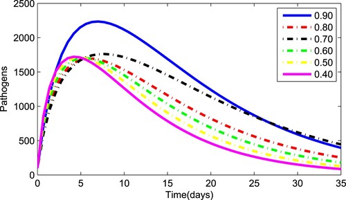
(1) ) for various values of the fractional parameter γ. Figure shows that the asymptomatic population decrease when the quantity of pathogen decreases. Figure describes the susceptible population's diminishing behaviour as γ increases. Similar results are obtained for hospitalized and quarantined classes shown in Figures and , respectively. Using the Caputo operator, Figure depicts the pandemic's long-term behaviour. At the conclusion of 50 days, the overall number of mild individuals seem to be decreasing. The significance of the order parameter γ for the pathogen class in the model is seen in Figure . The decrease in the values of γ has resulted in a considerable reduction in the number of infected people, as shown in Figure , and an increase in the numbers of infected people, as depicted in Figure .
Figure 3. Dynamics of Susceptible individuals for various values of fractional order and
.
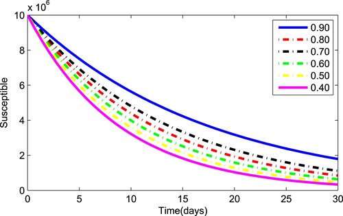
Figure 4. Dynamics of latent individuals for various values of fractional order and
.
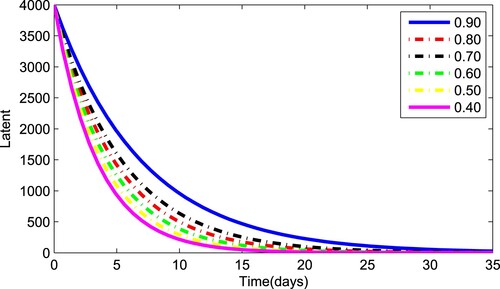
Figure 5. Dynamics of infected individuals for various values of fractional order and
.
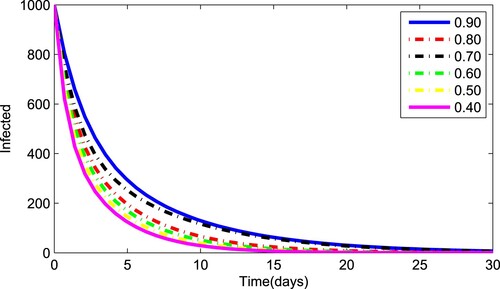
Figure 6. Dynamics of quarantined individuals for various values of fractional order and
.
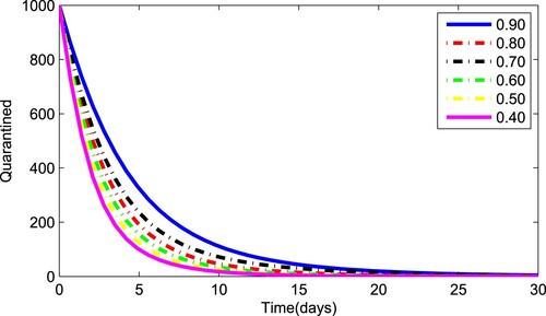
Figure 7. Dynamics of hospitalized individuals for various values of fractional order and
.
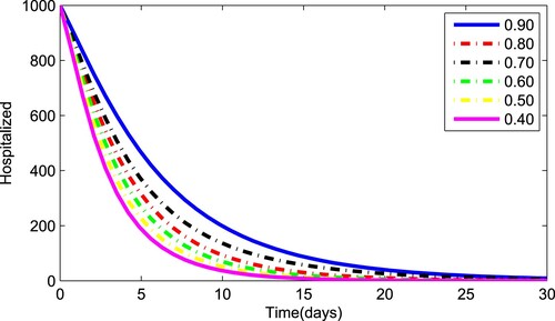
Figure 8. Dynamics of recovered individuals for various values of fractional order and
.
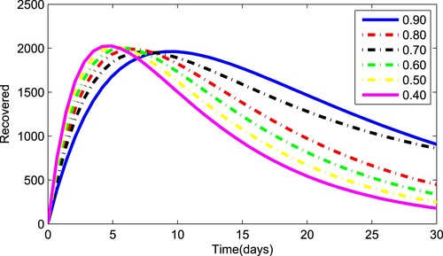
Figure 9. Dynamics of pathogen individuals for various values of fractional order and
.
10. Conclusion
The ongoing COVID-19 pandemic, lasting for more than two years now, remains one of the most significant challenges humanity has faced in combating coronavirus pathogens. The causative agent, SARS-CoV-2, possesses distinctive biological and transmission properties compared to its predecessors, SARS-CoV and MERS-CoV. Despite the implementation of numerous control strategies worldwide, the number of infected cases continues to rise, necessitating a deeper understanding of COVID-19's dynamics and the development of effective intervention measures. To gain insights into the transmission dynamics of COVID-19, a mathematical model called ‘’ is formulated and analysed in this study. This mathematical model aims to provide a comprehensive representation of the interaction between susceptible (
), latent (
), infected (
), quarantined infected (
), hospitalized infected (
), recovered (
), and deceased (
) individuals within the population. To ensure the validity and reliability of the model, its uniqueness and existence are established through the application of the Karsnoselskil's fixed-point theorem. Additionally, the basic reproduction number, denoted as
, is calculated using the next-generation matrices approach. This parameter provides crucial information about the disease's potential for spread and helps in determining the necessary control measures. The analysis of the model reveals both disease-free and endemic equilibrium points. It is proven that these equilibrium points are locally and globally asymptotically stable, indicating the stability of the system under certain conditions. Such insights are vital for understanding the long-term behavior of the COVID-19 transmission dynamics and devising appropriate strategies for disease control and containment. To visually represent the model's dynamics and gain a better understanding of the population's changes over time, graphical representations are employed. Different scenarios are considered by varying the value of the parameter γ, which is a measure of the recovery rate. These graphical representations enable researchers and policymakers to observe how the populations of susceptible, infected, quarantined, hospitalized, recovered, and deceased individuals evolve under different conditions of recovery rate. In conclusion, this study presents a comprehensive mathematical model for understanding the transmission dynamics of COVID-19. The analysis of this model, including the calculation of
and stability analysis of equilibrium points, contributes to a deeper understanding of the pandemic's behavior. The graphical representations further enhance the comprehension of population dynamics and can aid in devising effective strategies to control the spread of COVID-19 and mitigate its impact on communities worldwide.
Figure 10. Numerical solution of system (Equation1(1)
(1) ) with fractional order
.
![Figure 10. Numerical solution of system (Equation1(1) {0cDtγ[S]=σ−βSN(I+θL)−υS−πSP,0cDtγ[L]=βSN(I+θL)−(υ+ϖ+τ)L+πSP,0cDtγ[I]=τL−(υ+δ+υi+φ+α+ϕ)I,0cDtγ[Iq]=ϕI−(υ+ϵ+υq)Iq,0cDtγ[Ih]=φI−(υ+λ+υh)Ih,0cDtγ[R]=δI+ϖL+λIh+ϵIq−υR,0cDtγ[P]=αI−υpP,(1) ) with fractional order γ=0.90.](/cms/asset/ec334ddc-f4f9-439d-9f18-4be6c1749032/gipe_a_2326982_f0010_oc.jpg)
Figure 11. Numerical solution of system (Equation1(1)
(1) ) with fractional order
.
![Figure 11. Numerical solution of system (Equation1(1) {0cDtγ[S]=σ−βSN(I+θL)−υS−πSP,0cDtγ[L]=βSN(I+θL)−(υ+ϖ+τ)L+πSP,0cDtγ[I]=τL−(υ+δ+υi+φ+α+ϕ)I,0cDtγ[Iq]=ϕI−(υ+ϵ+υq)Iq,0cDtγ[Ih]=φI−(υ+λ+υh)Ih,0cDtγ[R]=δI+ϖL+λIh+ϵIq−υR,0cDtγ[P]=αI−υpP,(1) ) with fractional order γ=0.80.](/cms/asset/fe863d39-7b64-419e-854a-4b77e5d4253c/gipe_a_2326982_f0011_oc.jpg)
Figure 12. Numerical solution of system (Equation1(1)
(1) ) with fractional order
.
![Figure 12. Numerical solution of system (Equation1(1) {0cDtγ[S]=σ−βSN(I+θL)−υS−πSP,0cDtγ[L]=βSN(I+θL)−(υ+ϖ+τ)L+πSP,0cDtγ[I]=τL−(υ+δ+υi+φ+α+ϕ)I,0cDtγ[Iq]=ϕI−(υ+ϵ+υq)Iq,0cDtγ[Ih]=φI−(υ+λ+υh)Ih,0cDtγ[R]=δI+ϖL+λIh+ϵIq−υR,0cDtγ[P]=αI−υpP,(1) ) with fractional order γ=0.70.](/cms/asset/d358ef0b-5778-45d8-99c2-f3949b988f5a/gipe_a_2326982_f0012_oc.jpg)
Figure 13. Numerical solution of the system with fractional order .
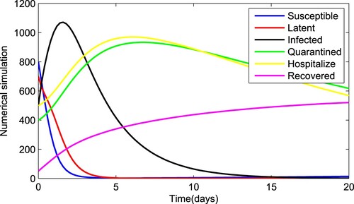
Figure 14. Numerical solution of system (Equation1(1)
(1) )with fractional order
.
![Figure 14. Numerical solution of system (Equation1(1) {0cDtγ[S]=σ−βSN(I+θL)−υS−πSP,0cDtγ[L]=βSN(I+θL)−(υ+ϖ+τ)L+πSP,0cDtγ[I]=τL−(υ+δ+υi+φ+α+ϕ)I,0cDtγ[Iq]=ϕI−(υ+ϵ+υq)Iq,0cDtγ[Ih]=φI−(υ+λ+υh)Ih,0cDtγ[R]=δI+ϖL+λIh+ϵIq−υR,0cDtγ[P]=αI−υpP,(1) )with fractional order γ=0.50.](/cms/asset/c5b25998-1bbd-4111-a9ea-5240421fb061/gipe_a_2326982_f0014_oc.jpg)
Figure 15. Numerical solution of system (Equation1(1)
(1) ) with fractional order
.
![Figure 15. Numerical solution of system (Equation1(1) {0cDtγ[S]=σ−βSN(I+θL)−υS−πSP,0cDtγ[L]=βSN(I+θL)−(υ+ϖ+τ)L+πSP,0cDtγ[I]=τL−(υ+δ+υi+φ+α+ϕ)I,0cDtγ[Iq]=ϕI−(υ+ϵ+υq)Iq,0cDtγ[Ih]=φI−(υ+λ+υh)Ih,0cDtγ[R]=δI+ϖL+λIh+ϵIq−υR,0cDtγ[P]=αI−υpP,(1) ) with fractional order γ=0.40.](/cms/asset/42fa6c98-2828-44fd-bb7e-a845718d913a/gipe_a_2326982_f0015_oc.jpg)
Figure 16. Numerical solution of system (Equation1(1)
(1) )with fractional order
.
![Figure 16. Numerical solution of system (Equation1(1) {0cDtγ[S]=σ−βSN(I+θL)−υS−πSP,0cDtγ[L]=βSN(I+θL)−(υ+ϖ+τ)L+πSP,0cDtγ[I]=τL−(υ+δ+υi+φ+α+ϕ)I,0cDtγ[Iq]=ϕI−(υ+ϵ+υq)Iq,0cDtγ[Ih]=φI−(υ+λ+υh)Ih,0cDtγ[R]=δI+ϖL+λIh+ϵIq−υR,0cDtγ[P]=αI−υpP,(1) )with fractional order γ=0.30.](/cms/asset/0ace3c58-72ac-4957-8dc6-0ebb1d54ff81/gipe_a_2326982_f0016_oc.jpg)
Authors' contributions
Authors approved the final manuscript.
Disclosure statement
No potential conflict of interest was reported by the author(s).
Data availability statement
Data sharing is not applicable to this paper as no datasets were generated or analysed during the current study.
Additional information
Funding
References
- Chen N, Zhou M, Dong X, et al. Epidemiological and clinical characteristics of 99 cases of 2019 novel coronavirus pneumonia in Wuhan, China: a descriptive study. The Lancet. 2020;395(10223):507–513. doi: 10.1016/S0140-6736(20)30211-7
- Covid C, Team R, COVID C, et al. Severe outcomes among patients with coronavirus disease 2019 (COVID-19) – United States, February 12–March 16, 2020. Morb Mortal Wkly Rep. 2020;69(12):343–346. doi: 10.15585/mmwr.mm6912e2
- Sherchan SP, Shahin S, Ward LM, et al. First detection of SARS-CoV-2 RNA in wastewater in North America: a study in Louisiana USA. Sci Total Environ. 2020;743:Article ID 140621. doi: 10.1016/j.scitotenv.2020.140621
- Agarwal P, Nieto JJ, Ruzhansky M, et al. Analysis of infectious disease problems (Covid-19) and their global impact. Springer; 2021.
- Zhao S, Chen H. Modeling the epidemic dynamics and control of COVID-19 outbreak in China. Quant Bio (Beijing, China). 2020;8(1):11–19.
- López M, Gallego C, Abós-Herrándiz R, et al. Impact of isolating COVID-19 patients in a supervised community facility on transmission reduction among household members. J Public Health. 2021;43(3):499–507. doi: 10.1093/pubmed/fdab002
- Khajanchi S, Sarkar K. Forecasting the daily and cumulative number of cases for the COVID-19 pandemic in India. Chaos: An Interdisciplinary J Nonlinear Sci. 2020;30(7):Article ID 071101. doi: 10.1063/5.0016240
- Zhang S, Diao M, Yu W, et al. Estimation of the reproductive number of novel coronavirus (COVID-19) and the probable outbreak size on the diamond princess cruise ship: a data-driven analysis. Int J Infect Dis. 2020;93:201–204. doi: 10.1016/j.ijid.2020.02.033
- Lin Q, Zhao S, Gao D, et al. A conceptual model for the coronavirus disease 2019 (COVID-19) outbreak in Wuhan, China with individual reaction and governmental action. Int J Infect Dis. 2020;93:211–216. doi: 10.1016/j.ijid.2020.02.058
- Yang C, Wang J. A mathematical model for the novel coronavirus epidemic in Wuhan, China. Math Biosci Eng: MBE. 2020;17(3):2708–2724. doi: 10.3934/mbe.2020148
- Sabatier J, Agrawal OP, Machado JT. Advances in fractional calculus. Vol. 4. Springer; 2007.
- Agarwal RP, Benchohra M, Hamani S. A survey on existence results for boundary value problems of nonlinear fractional differential equations and inclusions. Acta Appl Math. 2010;109(3):973–1033. doi: 10.1007/s10440-008-9356-6
- Diethelm K. The analysis of fractional differential equations: an application-oriented exposition using differential operators of Caputo type. Springer Science & Business Media; 2010.
- Ghaziani RK, Alidousti J, Eshkaftaki AB. Stability and dynamics of a fractional order Leslie–Gower prey–predator model. Appl Math Model. 2016;40(3):2075–2086. doi: 10.1016/j.apm.2015.09.014
- Ahmed I, Baba IA, Yusuf A, et al. Analysis of Caputo fractional-order model for COVID-19 with lockdown. Adv Differ Equ. 2020;2020(1):1–14. doi: 10.1186/s13662-019-2438-0
- Baba IA, Olamilekan LI, Yusuf A, et al. Analysis of meningitis model: a case study of northern Nigeria; 2020.
- Qureshi S, Yusuf A, Ali Shaikh A, et al. Mathematical modeling for adsorption process of dye removal nonlinear equation using power law and exponentially decaying kernels. Chaos: An Interdisciplinary J Nonlinear Sci. 2020;30(4):Article ID 043106. doi: 10.1063/1.5121845
- Zhang T, Li Y. Exponential Euler scheme of multi-delay Caputo–Fabrizio fractional-order differential equations. Appl Math Lett. 2022;124:Article ID 107709.
- Zhao K. Stability of a nonlinear ML-nonsingular kernel fractional Langevin system with distributed lags and integral control. Axioms. 2022;11(7):350. doi: 10.3390/axioms11070350
- Agarwal P, Deniz S, Jain S, et al. A new analysis of a partial differential equation arising in biology and population genetics via semi analytical techniques. Phys A: Stat Mech Appl. 2020;542:Article ID 122769. doi: 10.1016/j.physa.2019.122769
- Baleanu D, Jajarmi A, Mohammadi H, et al. A new study on the mathematical modelling of human liver with Caputo–Fabrizio fractional derivative. Chaos Solit Fractals. 2020;134:Article ID 109705. doi: 10.1016/j.chaos.2020.109705
- Tuan NH, Mohammadi H, Rezapour S. A mathematical model for COVID-19 transmission by using the Caputo fractional derivative. Chaos Solit Fractals. 2020;140:Article ID 110107. doi: 10.1016/j.chaos.2020.110107
- de Souza WM, Buss LF, da Silva Candido D, et al. Epidemiological and clinical characteristics of the COVID-19 epidemic in Brazil. Nat Hum Behav. 2020;4(8):856–865. doi: 10.1038/s41562-020-0928-4
- Baleanu D, Mohammadi H, Rezapour S. A fractional differential equation model for the COVID-19 transmission by using the Caputo–Fabrizio derivative. Adv Differ Equ. 2020;2020(1):1–27. doi: 10.1186/s13662-019-2438-0
- Zhao K. Existence, stability and simulation of a class of nonlinear fractional Langevin equations involving nonsingular Mittag–Leffler kernel. Fractal Fract. 2022;6(9):469. doi: 10.3390/fractalfract6090469
- Singh R, Abdeljawad T, Okyere E, et al. Modeling, analysis and numerical solution to malaria fractional model with temporary immunity and relapse. Adv Differ Equ. 2021;2021(1):1–27. doi: 10.1186/s13662-021-03506-6
- Daftardar-Gejji V. Fractional calculus and fractional differential equations. Springer; 2019.
- ul Rehman A, Singh R, Agarwal P. Modeling, analysis and prediction of new variants of covid-19 and dengue co-infection on complex network. Chaos Solit Fractals. 2021;150:Article ID 111008. doi: 10.1016/j.chaos.2021.111008
- Singh R, Tiwari P, Band SS, et al. Impact of quarantine on fractional order dynamical model of covid-19. Comput Biol Med. 2022;151:Article ID 106266. doi: 10.1016/j.compbiomed.2022.106266
- Chowdhury S, Chowdhury J, Ahmed SF, et al. Mathematical modelling of covid-19 disease dynamics: interaction between immune system and sars-cov-2 within host. AIMS Math. 2022;7(2):2618–2633. doi: 10.3934/math.2022147
- Kilbas A, Trujillo J. Differential equations of fractional order: methods, results and problems. ii. Appl Anal. 2002;81(2):435–493. doi: 10.1080/0003681021000022032
- Matignon D. Stability results for fractional differential equations with applications to control processing. In: Computational engineering in systems applications. Vol. 2. Citeseer; 1996. p. 963–968.
- Delavari H, Baleanu D, Sadati J. Stability analysis of Caputo fractional-order nonlinear systems revisited. Nonlinear Dyn. 2012;67(4):2433–2439. doi: 10.1007/s11071-011-0157-5
- Baba IA, Nasidi BA. Fractional order model for the role of mild cases in the transmission of COVID-19. Chaos Solit Fractals. 2021;142:Article ID 110374. doi: 10.1016/j.chaos.2020.110374