The use of Hermite wavelet collocation method for fractional cancer dynamical system

Abstract

Tumour is a very serious and dangerous health risk, which is defined as a mass or lump of tissue formalized by the aggregation of abnormal cells. In this paper, we have presented a comparative and chaotic investigation of tumour and effector cells using non-integer order tumour immune dynamical model. Also, we have looked at the interactions between different tumour cell populations and immunological composition using a model of a real-world medical research problem. Additionally, stability analysis of the proposed model is established with the help of fixed-point iteration. Further bifurcation diagrams, as well as phase portraits, have been used to study the proposed system numerically and to analyse its behaviour. For numerical simulations, we have used the Hermite wavelet operational matrix and Taufik-Atangana methods using Caputo fractional derivatives. models. The main objective of the paper is to convert nonlinear fractional systems into algebraic equations. Our findings will be valuable to biologists in cancer treatment.

Keywords:

• Cancer model
• chaotic behaviour
• Caputo derivative
• Laplace transform
• stability analysis
• bifurcation
• Hermite wavelet method
• numerical method

Mathematics Subject Classifications:

• 92-10
• 37-02
• 37N05

1. Introduction

Fractional calculus exemplifies the novel properties of disease models of arbitrary order. Fractional differential equations (FDEs) are utilized to describe a wide variety of phenomena in numerous scientific disciplines. Recent attention has been drawn to FDEs as a result of their wide range of applications in the applied sciences, including chaos theory, image processing, signal processing and system identification, and disease modelling. Many great works have been carried out at the modelling and manipulate the biological models by utilizing the fractional order differential equations [1–5]. The use of FDEs to solve disease models is more convenient than traditional integer-order mathematical modelling [6]. Many excellent studies have been done in the modelling and manipulation of biological models using FDEs. By employing Caputo derivatives in a computational manner, we were able to achieve the main purpose of the proposed work [7]. Dynamics is a time-evolutionary process that can be both deterministic and speculative. In general, a dynamical system is represented by a differential equation, and the related differential equation system is referred to as a dynamic system [8–13]. As a course in applied analysis, fractional calculus is a useful tool for modelling biological problems in science. It includes derivatives and integrals of any order [14, 15]. Non-integer models also allow study of past behaviour, while classical order derivative models only study present and future behaviour. The physical basis of fractional operators with differential memory is the widespread use of fractional calculus in mathematical modelling of evolutionary systems with memory effects on dynamics. Our motivation behind taking Caputo fractional operator is that we have operational matrix from Caputo derivatives [16, 17] and we don't have operational matrix of other derivatives, now in future we have to work on other derivatives. This is significant in demonstrating ancestral traits and memory performance as crucial roles in a variety of biological technologies.

The tumour is very serious and dangerous disease in medical science and it is defined as a mass or lump of tissue formalized by the aggregation of abnormal cells. In just a few days, it has become important to try to understand diseases with high mortality rates around the world, such as infectious diseases and cancer. A well-known non-integer order tumour-immune model is being used to study the dynamical behaviour. Chaos is the most widely cited example of nonlinear dynamics due to its extremely sensitive dependency on initial circumstances and parameter values. Nonlinear dynamical structures, as well as piecewise direct structures, can exhibit complete in-flight conduction. The study of mathematical models utilized in subjects such as physics, chemistry, biology, and economics is included in the study of dynamical systems [18]. Generalized fractional integral is nothing just only extension of classical fractional derivatives. One of the most common genetic illnesses is cancer [19, 20]. The disease is thought to be caused by mutations in cancer susceptibility genes [21]. The Caputo operator is used [22, 23] to examine a fractional order breast cancer model. Cancer is a disease that develops when deoxyribonucleic acid (DNA) damage occurs as a result of factors such as gender, age, heredity, lifestyle, malnutrition, stress, and cigarette and alcohol intake [24]. This condition, especially in its advanced stages, necessitates a lengthy treatment regimen. Because the number of people diagnosed with cancer or dying from it is increasing every day, it has been a popular research issue in recent years. There are a variety of malignancies that are commonly seen in acquired immunodeficiency syndrome (AIDS) patients. The main contribution of the paper is to obtain the wavelet operational matrix of fractional order using Hermite polynomials.

Mathematical modelling is a powerful tool for forecasting infectious disease dynamics in the field of applied sciences. In recent years, mathematical models have increasingly used fractional order differential and integral operators [25]. Due to their widespread use in [26, 27] fluid mechanics, economics, viscoelasticity, biology, physics, and engineering, numerous studies have been conducted using these models. The literature on modelling infectious diseases is rich, and several articles are published that use classical as well as fractional models [28]. More specifically, researchers use FOs to model bacterial diseases. An analysis of Coronavirus bacterial infection by Lei Zhang et al. For example, was carried out using fractional operators [29, 30]. The application of FDEs in nonlinear dynamics has recently spawned a slew of literature. This study investigated a non-integer cancer model that involved two immune effectors interacting with cancer cells. We give the non-integer cancer model, as well as the equilibrium points and conditions that ensure the steady local asymptotically stability. Also we have present a stable implicit method for solving the underlying differential fractional-order model. Fractional calculus, one of the most rapidly developing disciplines of mathematics, deals with arbitrary order derivatives and integrals. In numerous fields of science, FDEs have gotten a lot of attention. Memory qualities have been observed in many complicated processes in applied sciences. Because fractional derivatives have an extra degree of freedom, they can produce better results than integer derivatives. Indeed, in physics, chemistry, biology, and economics, FDEs have been successfully employed to represent events or processes having memory and hereditary features due to their inherent non-local property. Fractional calculus is a great tool for modelling memory and heredity materials and processes, as well as electrochemical difficulties.

Cancer tumour models range from simple mathematical equations to sophisticated computational simulations. There are two types of models: deterministic and stochastic. Biological processes are typically described by stochastic or deterministic models, which incorporate randomness and probability to account for uncertainties. For cancer researchers and clinicians, these studies provide insights into the underlying mechanisms driving tumour progression and assist in the development of more effective treatments.

Wavelet has been a popular mechanism in many research areas such as physical, chemical and computational sciences, image transformation biology, and many others in the last few decades. Since the 1980s, in wavelets often employed to solve DEs and integral DEs [31]. The primary goal of all wavelet based methods is to identify singularities, transient phenomena and irregular structure in the models investigated. Wavelet allows for the exact modelling of a wide range of operators and functions. As a result, wavelets play an important role in numerous domains. The wavelet basis is still in its early stages, although it has attracted attention for solving several types of FDEs with the method of Legendre wavelet method, Hermite wavelet method, and Bernoulli wavelet method [32, 33]. The wavelet transform is used to solve FDEs [34]. With the use of the Bernoulli wavelet, we solve system of fractional-order differential equations in paper [35, 36]. Haar wavelets will be utilized to solve the non-integer Lotka voltera model in 2020 [37]. Several research papers on Hermite wavelets for solving fractional differential equations are available. To the best of our knowledge, no article based on Hermite wavelet has been published for the purpose of solving biological models.

The main objective of the paper is to solve cancer model with fractional order α using operational matrix of Hermite wavelet approach. Compare the results using the other numerical method and different scenarios. The suggested model has not yet been solved using Hermite wavelet operational matrix, to the best of the author knowledge. In this paper, we focus on the Kumar et al. cancer paper [25], (1) $\begin{array}{rl}{}^C{D}_0^{\alpha }U\left(t\right)& =\mathrm{aU}\left(t\right)-r_{1}U\left(t\right)V\left(t\right)-r_{2}U\left(t\right)W\left(t\right),\\ {}^C{D}_0^{\alpha }V\left(t\right)& =-d_{1}V\left(t\right)+\frac{U^2\left(t\right)V\left(t\right)}{(U^2\left(t\right)+k_1)},\\ {}^C{D}_0^{\alpha }W\left(t\right)& =-d_{2}W\left(t\right)+\frac{U^2\left(t\right)W\left(t\right)}{(U^2\left(t\right)+k_2)},\end{array}$(1) under the initial conditions: (2) $(U_0,V_0,W_0)=(0.35,0.35,0.35),$(2) where $0<\alpha \le 1$, and ${}^C{D}_0^{\alpha }$ is the Caputo operator. $U\left(t\right)$, $V\left(t\right)$ and $W\left(t\right)$ are tumour cells, the immune effectors respectively. $a,r_1,r_2,d_1,d_2,k_1,k_2$ are the positive constants. Where a represent the improvement rate of tumour cells, $r_1,r_2$ represent reduction rates of tumour cells, and $d_1,d_2$ represent natural decay rate of the effectors cells $V\left(t\right)$ and $W\left(t\right)$. $k_1,k_2$ represent half saturation parameters. The parameters in this equation are all positive constants. In this model the main role of two effector cells such as cytotoxic T-cells, and natural killer cells and such effector cells interact with the cancer cells with response functional of Holling Type-III.

In the remainder of the paper, I have arranged it as follows. In Section 2, we discuss derivatives of non-integer order. An overview of the Hermite wavelet operational matrix is presented in Section 3. In Section 4, we present applications of Hermite wavelets and Toufik-Atangana numerical methods. Some Theorems and new idea are given in Section 5. Finally, numerical result and discussion of the non-integer order cancer model are given in Section 6. In Section 7 concludes with closing remarks.

2. Preliminaries

The section contains some brief preliminaries and notes regarding fractional calculus.

A natural number set is denoted by $\mathbb{N}$.

2.1. Definition 1. [38]

The (left sided) Riemann–Liouville non-integer order $\alpha >0$ of a function u is described by. (3) $I_0^{\alpha }u\left(t\right)=\frac{1}{\mathrm{\Gamma }\left(\alpha \right)}{\int }_0^t{(t-\xi )}^{\alpha -1}u\left(\xi \right)\mathrm{d}\xi ,t>0,$(3) here Γ represents Gamma function.

2.2. Definition 2 [38]

Let $0\le m-1<\alpha <m$, where $m\in \mathbb{N}$. The Caputo operator of a function u is described by. (4) $\begin{array}{rl}{}^C{D}_0^{\alpha }u\left(t\right)& =I_0^{m-\alpha }\left(\frac{{\mathrm{d}}^{m}u}{\mathrm{d}{t}^m}\right)\left(t\right),\\ {}^C{D}_0^{\alpha }u\left(t\right)& =\frac{1}{\mathrm{\Gamma }(m-\alpha )}{\int }_0^t{(t-\xi )}^{m-\alpha -1}\frac{{\mathrm{d}}^{m}u}{\mathrm{d}{\xi }^m}\left(\xi \right)\mathrm{d}\xi .\end{array}$(4) Basic properties of the system are as follows: ${}^C{D}_0^{\alpha }\left(I_0^{\alpha }u\right)\left(t\right)=u\left(t\right),$and $I_0^{\alpha }\left({}^C{D}_0^{\alpha }u\right)\left(t\right)=u\left(t\right)-\sum _{k=0}^{m-1}\frac{{\mathrm{d}}^{k}u}{\mathrm{d}{t}^k}\left(0^{+}\right)\frac{t^k}{k!}.$

3. The operational matrix of the Hermite wavelet function

The Hermite wavelets is denoted as ${\phi }_{\mathrm{nm}}\left(t\right)$, where $n=1,2,3,4,\dots 2^{k-1}$ and $m=0,1,2,3,\dots ,M-2,M-1$ is defined as $[0,t_l)$, (5) ${\phi }_{\mathrm{nm}}\left(t\right)=\{\begin{array}{ll}{\displaystyle \frac{2^{(k+1)\ast 0.5}}{\sqrt{\pi }}{\mathfrak{H}}_m(\frac{2^k}{t_l}t-2n+1),}& {\displaystyle \frac{2n-2}{2^k}{t}_l\le t<\frac{2n}{2^k}{t}_l}\\ 0,& \mathrm{otherwise},\end{array}$(5) here M, k are nonnegative integer and ${\mathfrak{H}}_m\left(t\right)$ is known as degree m Hermite polynomial with respect of weight function $w\left(t\right)=\sqrt{1-t^2}$ on the real axis and fulfils the following recurrence relationship. $\begin{array}{rl}{\mathfrak{H}}_0\left(t\right)& =1,\\ {\mathfrak{H}}_1\left(t\right)& =2t,\\ {\mathfrak{H}}_{m+2}\left(t\right)& =2t{\mathfrak{H}}_{m+1}\left(t\right)-2(m+1){\mathfrak{H}}_m\left(t\right).\end{array}$For ${\phi }_{\mathrm{nm}}$, let ${\mathrm{\Theta }}_{k,M}$ be the space spanned by the Hermite wavelet, defined as ${\mathrm{\Theta }}_{k,M}=\mathrm{span}\{{\phi }_{1,0},\dots ,{\phi }_{2^{k-1},0},{\phi }_{2,1},\dots ,{\phi }_{2^{k-1},1},\dots ,{\phi }_{2^{k-1},2},\dots ,{\phi }_{2^{k-1},M}\}\subseteq L^2(0,1).$Suppose ℏ be an arbitrary element in $L^2(0,1)$. Then we have approximation such as ${\hslash }_0\in {\mathrm{\Theta }}_{k,M}$, $\mathrm{\forall \Re }\in {\mathrm{\Theta }}_{k,M},\Vert \hslash -{\hslash }_0\Vert \le \Vert \hslash -\mathrm{\Re }\Vert .$Since ${\hslash }_0\in {\mathrm{\Theta }}_{k,M}$ is the unique approximation then ∃ unique coefficients $\mathrm{\Xi }{O}_{1,0},\dots ,\mathrm{\Xi }{O}_{2^{k-1},0},..,\mathrm{\Xi }{O}_{2^{k-1},1},\mathrm{\Xi }{O}_{2,2},\dots .,\mathrm{\Xi }{O}_{2^{k-1},2},\dots ,\mathrm{\Xi }{O}_{2^{k-1},M}$ as a result (6) $\hslash \left(t\right)\approx {\hslash }_0\left(t\right)=\sum _{n=1}^{2^{k-1}}\sum _{m=0}^{M-1}\mathrm{\Xi }{O}_{\mathrm{nm}}{\phi }_{\mathrm{nm}}\left(t\right)=\mathrm{\Xi }{O}^{T}G,$(6) where $\mathrm{\Xi }O$ and G vectors are follows as $\begin{array}{rl}\mathrm{\Xi }{O}^T& =[\mathrm{\Xi }{O}_{1,0},\dots ,\mathrm{\Xi }{O}_{2^{k-1},0},\mathrm{\Xi }{O}_{1,1},\dots ,\\ & \mathrm{\Xi }{O}_{2^{k-1},1},\mathrm{\Xi }{O}_{2,2},\dots ,\mathrm{\Xi }{O}_{2^{k-1},2},\dots ,\mathrm{\Xi }{O}_{2^{k-1},M-1}],\end{array}$and $G^T=[{\phi }_{1,0},{\phi }_{2,0},{\phi }_{3,0},\dots ,{\phi }_{2^{k-1},0},{\phi }_{1,1},{\phi }_{2,1},\dots ,{\phi }_{2^{k-1},1},{\phi }_{2,2},\dots ,{\phi }_{2^{k-1},2},\dots ,{\phi }_{2^{k-1},M-1}].$Let us take M = 3, k = 2 and have wavelet collocation point defined as $t_i=\frac{2i-1}{2\hat{m}},i=1,2,3,\dots \hat{m}=$ $2^{k-1}M$, after that we get operational matrix of Hermite wavelet ${\varphi }_{6\ast 6}=\left[\begin{array}{cccccc}1.598& 1.598& 1.598& 0& 0& 0\\ 0& 0& 0& 1.598& 1.598& 1.598\\ -2.1277& 0& 2.1277& 0& 0& 0\\ 0& 0& 0& -2.1277& 0& 2.1277\\ -0.3546& -3.1915& -0.3546& 0& 0& 0\\ 0& 0& 0& -0.3546& -3.1915& -0.3546\end{array}\right]$finally, we have obtained $6\times 6$ Hermite wavelet matrix.

3.1. The operational matrix of the Hermite wavelet

Integer and non-integer order integration using the Hermite wavelet operational matrix is presented next. These operational matrices are extremely important in the proposed strategy for resolving the problem.

3.2. Basic properties of block pulse functions $($ BPFs $)$

In the $[0,t_l)$ we have defined BPFs $B_j\left(t\right)=\{\begin{array}{ll}1& {\displaystyle \frac{j{t}_l}{\hat{m}}\le t<\frac{(j+1)t_l}{\hat{m}},}\\ 0& \mathrm{otherwise},\end{array}$here $B_{\hat{m}}=[b_1,b_2,\dots ,b_{m-1},b_m]$ and $j=0,1,2,3,\dots .,\hat{m}$. The BPFs useful features are stated in this work, and we will utilize it to build the operational matrix of Hermite wavelet of arbitrary order. $\begin{array}{rl}\left(I_t^{\alpha }{B}_{\hat{m}}\right)\left(t\right)& \cong F^{\alpha }{B}_{\hat{m}},\\ F_{m\ast m}^{\alpha }& =\frac{t_l^{\alpha }}{{\hat{m}}^{\alpha }\mathrm{\Gamma }(\alpha +2)}\left[\begin{array}{cccccccc}1& {\varsigma }_1& {\varsigma }_2& {\varsigma }_3& {\varsigma }_4& \cdots & \cdots & {\varsigma }_{\hat{m}-1}\\ 0& 1& {\varsigma }_1& {\varsigma }_2& {\varsigma }_3& \cdots & \cdots & {\varsigma }_{\hat{m}-2}\\ 0& 0& 1& {\varsigma }_1& {\varsigma }_2& \cdots & \cdots & {\varsigma }_{\hat{m}-3}\\ 0& 0& 0& 1& {\varsigma }_1& \cdots & \cdots & {\varsigma }_{\hat{m}-4}\\ ⋮& ⋮& ⋮& ⋮& \ddots & \ddots & & ⋮\\ ⋮& ⋮& ⋮& ⋮& & \ddots & & ⋮\\ 0& 0& \cdots & \cdots & 0& 0& 1& {\varsigma }_1\\ 0& 0& \cdots & \cdots & 0& 0& 0& 1\end{array}\right],\end{array}$here ${\varsigma }_l=(l+1{)}^{\alpha +1}-2l^{\alpha +1}+(l-1{)}^{\alpha +1}$, where $l=1,2,\dots ,\hat{m}-1$. We are presently creating the operational matrix of Hermite wavelet for arbitrary order integration $P^{\alpha }$. Now we have: $\left(I_t^{\alpha }\phi \right)\left(t\right)\cong P^{\alpha }\phi \left(t\right).$After that we have: $\left(I_t^{\alpha }\phi \right)\left(t\right)\cong \left(I_t^{\alpha }\phi B_{\hat{m}}\right)\left(t\right)=\phi \left(I_t^{\alpha }{B}_{\hat{m}}\right)\left(t\right)\approx \phi F^{\alpha }{B}_{\hat{m}}.$There for, $\begin{array}{rl}{P}^{\alpha }\phi \left(t\right)& \cong \phi \left(t\right)F^{\alpha }{B}_{\hat{m}}\\ P^{\alpha }& ={\varphi }_{\hat{m}\times \hat{m}}{F}^{\alpha }{\varphi }_{\hat{m}\times \hat{m}}^{-1}.\end{array}$We get the operational matrix $P^{\alpha }$, using the above manner, where $\alpha =0.90,M=3,k=2$ and $t_l=1$ is given as follows as: $P_{6\times 6}^{0.90}=\left[\begin{array}{cccccc}0.2899& 0.5105& 0.1363& -0.0158& -0.0041& 0.0031\\ 0& 0.2899& 0& 0.1363& 0& -0.0041\\ -0.0994& 0.0206& 0.0219& -0.0066& 0.0763& 0.0023\\ 0& -0.0944& 0& 0.0219& 0& 0.0763\\ -0.2292& -0.4133& -0.1563& 0.0115& 0.0115& -0.0019\\ 0& -0.2292& 0& -0.1563& 0& 0.0155\end{array}\right]$finally, we have obtained operational matrix $P^{\alpha }$ of arbitrary order $\alpha =0.90$.

4. A description of the proposed method

4.1. The primary objective of this section is to use the Toufik–Atangana method [39] and the Hermite wavelet approach to create a fractional cancer model.

In this section, we will use a Toufik-Atangana method to solve the non-integer order cancer model (1(1) $\begin{array}{rl}{}^C{D}_0^{\alpha }U\left(t\right)& =\mathrm{aU}\left(t\right)-r_{1}U\left(t\right)V\left(t\right)-r_{2}U\left(t\right)W\left(t\right),\\ {}^C{D}_0^{\alpha }V\left(t\right)& =-d_{1}V\left(t\right)+\frac{U^2\left(t\right)V\left(t\right)}{(U^2\left(t\right)+k_1)},\\ {}^C{D}_0^{\alpha }W\left(t\right)& =-d_{2}W\left(t\right)+\frac{U^2\left(t\right)W\left(t\right)}{(U^2\left(t\right)+k_2)},\end{array}$(1) )–(2(2) $(U_0,V_0,W_0)=(0.35,0.35,0.35),$(2) ).

We can discuss as follow: (7) $\{\begin{array}{l}{}_a^C{D}_t^{\alpha }U\left(t\right)=\mathrm{aU}\left(t\right)-r_{1}U\left(t\right)V\left(t\right)-r_{2}U\left(t\right)W\left(t\right),\\ {}_a^C{D}_t^{\alpha }V\left(t\right)=-d_{1}V\left(t\right)+{\displaystyle \frac{{\left(U\left(t\right)\right)}^{2}V\left(t\right)}{({\left(U\left(t\right)\right)}^2+k_1)},}\\ {}_a^C{D}_t^{\alpha }W\left(t\right)=-d_{2}W\left(t\right)+{\displaystyle \frac{{\left(U\left(t\right)\right)}^{2}W\left(t\right)}{({\left(U\left(t\right)\right)}^2+k_2)}.}\end{array}$(7) We convert Equation (7(7) $\{\begin{array}{l}{}_a^C{D}_t^{\alpha }U\left(t\right)=\mathrm{aU}\left(t\right)-r_{1}U\left(t\right)V\left(t\right)-r_{2}U\left(t\right)W\left(t\right),\\ {}_a^C{D}_t^{\alpha }V\left(t\right)=-d_{1}V\left(t\right)+{\displaystyle \frac{{\left(U\left(t\right)\right)}^{2}V\left(t\right)}{({\left(U\left(t\right)\right)}^2+k_1)},}\\ {}_a^C{D}_t^{\alpha }W\left(t\right)=-d_{2}W\left(t\right)+{\displaystyle \frac{{\left(U\left(t\right)\right)}^{2}W\left(t\right)}{({\left(U\left(t\right)\right)}^2+k_2)}.}\end{array}$(7) ),

where ${}_a^C{D}_t^{\alpha }$ this well-known fractional operator is called Caputo, assume the equation above is.

Further, integrating Equation (7(7) $\{\begin{array}{l}{}_a^C{D}_t^{\alpha }U\left(t\right)=\mathrm{aU}\left(t\right)-r_{1}U\left(t\right)V\left(t\right)-r_{2}U\left(t\right)W\left(t\right),\\ {}_a^C{D}_t^{\alpha }V\left(t\right)=-d_{1}V\left(t\right)+{\displaystyle \frac{{\left(U\left(t\right)\right)}^{2}V\left(t\right)}{({\left(U\left(t\right)\right)}^2+k_1)},}\\ {}_a^C{D}_t^{\alpha }W\left(t\right)=-d_{2}W\left(t\right)+{\displaystyle \frac{{\left(U\left(t\right)\right)}^{2}W\left(t\right)}{({\left(U\left(t\right)\right)}^2+k_2)}.}\end{array}$(7) ), we get: (8) $\{\begin{array}{l}{}_a^C{D}_t^{\alpha }U\left(t\right)={\mathrm{\Psi }}_1(U,V,W,t),\\ {}_a^C{D}_t^{\alpha }V\left(t\right)={\mathrm{\Psi }}_2(U,V,W,t),\\ {}_a^C{D}_t^{\alpha }W\left(t\right)={\mathrm{\Psi }}_3(U,V,W,t).\end{array}$(8) At point $t=t_{n+1}$, (9) $\{\begin{array}{l}U\left(t_{n+1}\right)=U\left(0\right)+{\displaystyle \frac{1}{\mathrm{\Gamma }\alpha }{\int }_0^{t_{n+1}}{\mathrm{\Psi }}_1(U,V,W,\tau ){(t_{n+1}-\tau )}^{\alpha -1}\mathrm{d}\xi ,}\\ V\left(t_{n+1}\right)=V\left(0\right)+{\displaystyle \frac{1}{\mathrm{\Gamma }\alpha }{\int }_0^{t_{n+1}}{\mathrm{\Psi }}_2(U,V,W,\tau ){(t_{n+1}-\tau )}^{\alpha -1}\mathrm{d}\xi ,}\\ W\left(t_{n+1}\right)=W\left(0\right)+{\displaystyle \frac{1}{\mathrm{\Gamma }\alpha }{\int }_0^{t_{n+1}}{\mathrm{\Psi }}_3(U,V,W,\tau ){(t_{n+1}-\tau )}^{\alpha -1}\mathrm{d}\xi ,}\end{array}$(9) furthermore we get the following equation, (10) $\{\begin{array}{l}U\left(t_{n+1}\right)=U\left(0\right)+{\displaystyle \frac{1}{\mathrm{\Gamma }\alpha }\sum _{j=2}^n{\int }_{t_j}^{t_{j+1}}{\mathrm{\Psi }}_1(U,V,W,\xi ){(t_{n+1}-\xi )}^{\alpha -1}\mathrm{d}\xi ,}\\ V\left(t_{n+1}\right)=V\left(0\right)+{\displaystyle \frac{1}{\mathrm{\Gamma }\alpha }\sum _{j=2}^n{\int }_{t_j}^{t_{j+1}}{\mathrm{\Psi }}_2(U,V,W,\xi ){(t_{n+1}-\xi )}^{\alpha -1}\mathrm{d}\xi ,}\\ W\left(t_{n+1}\right)=W\left(0\right)+{\displaystyle \frac{1}{\mathrm{\Gamma }\alpha }\sum _{j=2}^n{\int }_{t_j}^{t_{j+1}}{\mathrm{\Psi }}_3(U,V,W,\xi ){(t_{n+1}-\xi )}^{\alpha -1}\mathrm{d}\xi .}\end{array}$(10) Apply two step Lagrange polynomial piece wise interpolation on the expression, say ${\mathrm{\Psi }}_1(U,V,W,t),{\mathrm{\Psi }}_2(U,V,W,t)\mathrm{and}{\mathrm{\Psi }}_3(U,V,W,t)$ are involved in Equation (10(10) $\{\begin{array}{l}U\left(t_{n+1}\right)=U\left(0\right)+{\displaystyle \frac{1}{\mathrm{\Gamma }\alpha }\sum _{j=2}^n{\int }_{t_j}^{t_{j+1}}{\mathrm{\Psi }}_1(U,V,W,\xi ){(t_{n+1}-\xi )}^{\alpha -1}\mathrm{d}\xi ,}\\ V\left(t_{n+1}\right)=V\left(0\right)+{\displaystyle \frac{1}{\mathrm{\Gamma }\alpha }\sum _{j=2}^n{\int }_{t_j}^{t_{j+1}}{\mathrm{\Psi }}_2(U,V,W,\xi ){(t_{n+1}-\xi )}^{\alpha -1}\mathrm{d}\xi ,}\\ W\left(t_{n+1}\right)=W\left(0\right)+{\displaystyle \frac{1}{\mathrm{\Gamma }\alpha }\sum _{j=2}^n{\int }_{t_j}^{t_{j+1}}{\mathrm{\Psi }}_3(U,V,W,\xi ){(t_{n+1}-\xi )}^{\alpha -1}\mathrm{d}\xi .}\end{array}$(10) ) as given below, (11) $\{\begin{array}{l}{Q}_j\left(\xi \right)={\displaystyle \frac{\xi -t_{j-1}}{t_j-t_{j-1}}{\mathrm{\Psi }}_1(U_j,V_j,W_j,{\xi }_j)-{\displaystyle \frac{\xi -t_j}{t_j-t_{j-1}}{\mathrm{\Psi }}_1(U_{j-1},V_{j-1},W_{j-1},{\xi }_{j-1}),}}\\ R_j\left(\xi \right)={\displaystyle \frac{\xi -t_{j-1}}{t_j-t_{j-1}}{\mathrm{\Psi }}_2(U_j,V_j,W_j,{\xi }_j)-{\displaystyle \frac{\xi -t_j}{t_j-t_{j-1}}{\mathrm{\Psi }}_2(U_{j-1},V_{j-1},W_{j-1},{\xi }_{j-1}),}}\\ S_j\left(\xi \right)={\displaystyle \frac{\xi -t_{j-1}}{t_j-t_{j-1}}{\mathrm{\Psi }}_3(U_j,V_j,W_j,{\xi }_j)-{\displaystyle \frac{\xi -t_j}{t_j-t_{j-1}}{\mathrm{\Psi }}_3(U_{j-1},V_{j-1},W_{j-1},{\xi }_{j-1}).}}\end{array}$(11) Using the above approximation, the following process can be developed: (12) $\{\begin{array}{l}U\left(t_{n+1}\right)=U\left(0\right)+{\displaystyle \frac{1}{\mathrm{\Gamma }\alpha }\sum _{j=0}^n{\int }_{t_j}^{t_{j+1}}{(t_{n+1}-\xi )}^{\alpha -1}{Q}_j\left(\xi \right)\mathrm{d}\xi ,}\\ V\left(t_{n+1}\right)=V\left(0\right)+{\displaystyle \frac{1}{\mathrm{\Gamma }\alpha }\sum _{j=0}^n{\int }_{t_j}^{t_{j+1}}{(t_{n+1}-\xi )}^{\alpha -1}{R}_j\left(\xi \right)\mathrm{d}\xi ,}\\ W\left(t_{n+1}\right)=W\left(0\right)+{\displaystyle \frac{1}{\mathrm{\Gamma }\alpha }\sum _{j=0}^n{\int }_{t_j}^{t_{j+1}}{(t_{n+1}-\xi )}^{\alpha -1}{S}_j\left(\xi \right)\mathrm{d}\xi .}\end{array}$(12) And, now we have, (13) $\{\begin{array}{l}U\left(t_{n+1}\right)=U\left(0\right)+{\displaystyle \frac{1}{\mathrm{\Gamma }\alpha }{\displaystyle \sum _{j=0}^n(\frac{{\mathrm{\Psi }}_1(U_j,V_j,W_j,{\xi }_j)}{h}{\int }_{t_j}^{t_{j+1}}(\xi -t_{j-1}){(t_{n+1}-\xi )}^{\alpha -1}\mathrm{d}\xi ,}}\\ {\displaystyle -\frac{{\mathrm{\Psi }}_1(U_{j-1},V_{j-1},W_{j-1},{\xi }_{j-1})}{h}{\int }_{t_j}^{t_{j+1}}(\xi -t_j){(t_{n+1}-\xi )}^{\alpha -1}\mathrm{d}\xi ),}\\ V\left(t_{n+1}\right)=V\left(0\right)+{\displaystyle \frac{1}{\mathrm{\Gamma }\alpha }{\displaystyle \sum _{j=0}^n(\frac{{\mathrm{\Psi }}_1(U_j,V_j,W_j,{\xi }_j)}{h}{\int }_{t_j}^{t_{j+1}}(\xi -t_{j-1}){(t_{n+1}-\xi )}^{\alpha -1}\mathrm{d}\xi ,}}\\ {\displaystyle -\frac{{\mathrm{\Psi }}_1(U_{j-1},V_{j-1},W_{j-1},{\xi }_{j-1})}{h}{\displaystyle {\int }_{t_j}^{t_{j+1}}(\xi -t_j){(t_{n+1}-\xi )}^{\alpha -1}\mathrm{d}\xi ),}}\\ W\left(t_{n+1}\right)=W\left(0\right)+{\displaystyle \frac{1}{\mathrm{\Gamma }\alpha }{\displaystyle \sum _{j=0}^n(\frac{{\mathrm{\Psi }}_1(U_j,V_j,W_j,{\xi }_j)}{h}{\int }_{t_j}^{t_{j+1}}(\xi -t_{j-1}){(t_{n+1}-\xi )}^{\alpha -1}\mathrm{d}\xi ,}}\\ {\displaystyle -\frac{{\mathrm{\Psi }}_1(U_{j-1},V_{j-1},W_{j-1},{\xi }_{j-1})}{h}{\displaystyle {\int }_{t_j}^{t_{j+1}}(\xi -t_j){(t_{n+1}-\xi )}^{\alpha -1}\mathrm{d}\xi ).}}\end{array}$(13) For above integrals, we can define as: $\{\begin{array}{l}{A}_{\alpha ,k,1}={\int }_{t_k}^{t_{k+1}}(\xi -t_{k-1}){(t_{n+1}-\xi )}^{\alpha -1}\mathrm{d}\xi ,\\ ={\displaystyle \frac{h^{\alpha +1}{(n+1-k)}^{\alpha }(n-k+2+\alpha )-{(n-k)}^{\alpha }(n-k+2+2\alpha )}{\alpha (\alpha +1)},}\\ A_{\alpha ,k,2}={\displaystyle {\int }_{t_k}^{t_{k+1}}(\xi -t_k){(t_{n+1}-\xi )}^{\alpha -1}\mathrm{d}\xi ,}\\ ={\displaystyle \frac{h^{\alpha +1}{(n+1-k)}^{\alpha +1}-{(n-k)}^{\alpha }(n-k+1+\alpha )}{\alpha (\alpha +1)}.}\end{array}$We discussed the numerical scheme for Caputo operator as, (14) $\{\begin{array}{l}U\left(t_{n+1}\right)=U\left(0\right)+{\displaystyle \frac{1}{\mathrm{\Gamma }\alpha }\sum _{j=0}^n\left(\frac{h^{\alpha }{\mathrm{\Psi }}_1(U_j,V_j,W_j,t_j)}{\mathrm{\Gamma }\alpha +2}\right((n+1-j{)}^{\alpha },}\\ \times (n-j+2+\alpha )-{(n-j)}^{\alpha }(n-j+2+2\alpha ))-{\displaystyle \frac{h^{\alpha }{\mathrm{\Psi }}_1(U_j,V_{j-1},W_{j-1},t_{j-1})}{\mathrm{\Gamma }\alpha +2},}\\ ({(n+1-j)}^{\alpha +1}-{(n-j)}^{\alpha }(n-j+1+\alpha ))+I_{1n}^{\alpha },\\ V\left(t_{n+1}\right)=V\left(0\right)+{\displaystyle \frac{1}{\mathrm{\Gamma }\alpha }\sum _{j=0}^n\left(\frac{h^{\alpha }{\mathrm{\Psi }}_2(U_j,V_j,W_j,t_j)}{\mathrm{\Gamma }\alpha +2}\right((n+1-j{)}^{\alpha },}\\ \times (n-j+2+\alpha )-{(n-j)}^{\alpha }(n-j+2+2\alpha ))-{\displaystyle \frac{h^{\alpha }{\mathrm{\Psi }}_2(U_j,V_{j-1},W_{j-1},t_{j-1})}{\mathrm{\Gamma }\alpha +2},}\\ ({(n+1-j)}^{\alpha +1}-{(n-j)}^{\alpha }(n-j+1+\alpha ))+I_{2n}^{\alpha },\\ W\left(t_{n+1}\right)=W\left(0\right)+{\displaystyle \frac{1}{\mathrm{\Gamma }\alpha }\sum _{j=0}^n\left(\frac{h^{\alpha }{\mathrm{\Psi }}_3(U_j,V_j,W_j,t_j)}{\mathrm{\Gamma }\alpha +2}\right((n+1-j{)}^{\alpha },}\\ \times (n-j+2+\alpha )-{(n-j)}^{\alpha }(n-j+2+2\alpha ))-{\displaystyle \frac{h^{\alpha }{\mathrm{\Psi }}_3(U_j,V_{j-1},W_{j-1},t_{j-1})}{\mathrm{\Gamma }\alpha +2},}\\ ({(n+1-j)}^{\alpha +1}-{(n-j)}^{\alpha }(n-j+1+\alpha ))+I_{3n}^{\alpha }.\end{array}$(14) Where (15) $\{\begin{array}{l}{I}_{1n}^{\alpha }={\displaystyle \frac{1}{\mathrm{\Gamma }\alpha }\sum _{j=0}^n{\int }_{t_j}^{t_{j-1}}{\displaystyle \frac{(\xi -t_j)(\xi -t_{j-1})}{2!}\frac{{\mathrm{\partial }}^2}{\mathrm{\partial }{\xi }^2}{\left[{\mathrm{\Psi }}_1(U,V,W,\xi )\right]}_{\mu =c_j}{(t_{n+1}-\xi )}^{\alpha -1}\mathrm{d}\xi ,}}\\ I_{2n}^{\alpha }={\displaystyle \frac{1}{\mathrm{\Gamma }\alpha }\sum _{j=0}^n{\int }_{t_j}^{t_{j-1}}{\displaystyle \frac{(\xi -t_j)(\xi -t_{j-1})}{2!}\frac{{\mathrm{\partial }}^2}{\mathrm{\partial }{\xi }^2}{\left[{\mathrm{\Psi }}_2(U,V,W,\xi )\right]}_{\mu =c_j}{(t_{n+1}-\xi )}^{\alpha -1}\mathrm{d}\xi ,}}\\ I_{3n}^{\alpha }={\displaystyle \frac{1}{\mathrm{\Gamma }\alpha }\sum _{j=0}^n{\int }_{t_j}^{t_{j-1}}{\displaystyle \frac{(\xi -t_j)(\xi -t_{j-1})}{2!}\frac{{\mathrm{\partial }}^2}{\mathrm{\partial }{\xi }^2}{\left[{\mathrm{\Psi }}_3(U,V,W,\xi )\right]}_{\mu =c_j}{(t_{n+1}-\xi )}^{\alpha -1}\mathrm{d}\xi .}}\end{array}$(15)

4.2. Hermite wavelet method for the Ccancer model with non-integer order

The Hermite wavelet approach is applied to the non-integer order cancer model in this subsection. Here we have: (16) $\{\begin{array}{l}{}_a^C{D}_t^{\alpha }U\left(t\right){=}^1\mathrm{\Xi }{O}^T{G}_{\hat{m}}\left(t\right),\\ {}_a^C{D}_t^{\alpha }V\left(t\right)={}^2\mathrm{\Xi }{O}^T{G}_{\hat{m}}\left(t\right),\\ {}_a^C{D}_t^{\alpha }W\left(t\right)={}^3\mathrm{\Xi }{O}^T{G}_{\hat{m}}\left(t\right),\end{array}$(16) where, $\begin{array}{rl}{}^1\mathrm{\Xi }O& ={[}^1\mathrm{\Xi }{O}_{1,0},\dots {,}^1\mathrm{\Xi }{O}_{2^{k-1},0}{,}^1\mathrm{\Xi }{O}_{1,1}{,}^1\mathrm{\Xi }{O}_{2,1},\dots {,}^1\mathrm{\Xi }{O}_{2^{k-1},1}{,}^1\mathrm{\Xi }{O}_{2,2},\\ & \dots {,}^1\mathrm{\Xi }{O}_{2^{k-1},2},\dots \\ & ,{}^1\mathrm{\Xi }{O}_{2^{k-1},M-1}]\\ {}^2\mathrm{\Xi }O& ={[}^2\mathrm{\Xi }{O}_{1,0}{,}^2\mathrm{\Xi }{O}_{2,0}{,}^2\mathrm{\Xi }{O}_{3,0},\\ & \dots {,}^2\mathrm{\Xi }{O}_{2^{k-1},0}{,}^2\mathrm{\Xi }{O}_{1,1}{,}^2\mathrm{\Xi }{O}_{2,1},\dots {,}^2\mathrm{\Xi }{O}_{2^{k-1},1}{,}^2\mathrm{\Xi }{O}_{2,2},\dots \\ & ,{}^2\mathrm{\Xi }{O}_{2^{k-1},2},\dots {,}^2\mathrm{\Xi }{O}_{2^{k-1},M-1}]\\ {}^3\mathrm{\Xi }O& ={[}^3\mathrm{\Xi }{O}_{1,0}{,}^3\mathrm{\Xi }{O}_{2,0}{,}^3\mathrm{\Xi }{O}_{3,0},\dots {,}^3\mathrm{\Xi }{O}_{2^{k-1},0}{,}^3\mathrm{\Xi }{O}_{1,1}{,}^3\mathrm{\Xi }{O}_{2,1},\\ & \dots {,}^3\mathrm{\Xi }{O}_{2^{k-1},1}{,}^3\mathrm{\Xi }{O}_{2,2},\dots \\ & ,{}^3\mathrm{\Xi }{O}_{2^{k-1},2},\dots {,}^3\mathrm{\Xi }{O}_{2^{k-1},M-1}]\end{array}$are the unidentified vectors, and $G_{\hat{m}}$ vector have been taken above sides. Furthermore, applying the R-L integral, and use (1(1) $\begin{array}{rl}{}^C{D}_0^{\alpha }U\left(t\right)& =\mathrm{aU}\left(t\right)-r_{1}U\left(t\right)V\left(t\right)-r_{2}U\left(t\right)W\left(t\right),\\ {}^C{D}_0^{\alpha }V\left(t\right)& =-d_{1}V\left(t\right)+\frac{U^2\left(t\right)V\left(t\right)}{(U^2\left(t\right)+k_1)},\\ {}^C{D}_0^{\alpha }W\left(t\right)& =-d_{2}W\left(t\right)+\frac{U^2\left(t\right)W\left(t\right)}{(U^2\left(t\right)+k_2)},\end{array}$(1) )–(2(2) $(U_0,V_0,W_0)=(0.35,0.35,0.35),$(2) ), we obtain: (17) $\{\begin{array}{ll}\left(I_0^{\mathrm{\alpha C}}{D}_0^{\alpha }\right)U\left(t\right)=U\left(t\right)-U_0=U\left(t\right)-\delta =& {}^1\mathrm{\Xi }{O}^T{P}^{\alpha }{G}_{\hat{m}}\left(t\right),\\ \left(I_0^{\mathrm{\alpha C}}{D}_0^{\alpha }\right)V\left(t\right)=V\left(t\right)-V_0=V\left(t\right)-\gamma =& {}^2\mathrm{\Xi }{O}^T{P}^{\alpha }{G}_{\hat{m}}\left(t\right),\\ \left(I_0^{\mathrm{\alpha C}}{D}_0^{\alpha }\right)W\left(t\right)=W\left(t\right)-W_0=W\left(t\right)-\varrho =& {}^3\mathrm{\Xi }{O}^T{P}^{\alpha }{G}_{\hat{m}}\left(t\right),\end{array}$(17) where $P^{\alpha }$ is given above. Putting (16(16) $\{\begin{array}{l}{}_a^C{D}_t^{\alpha }U\left(t\right){=}^1\mathrm{\Xi }{O}^T{G}_{\hat{m}}\left(t\right),\\ {}_a^C{D}_t^{\alpha }V\left(t\right)={}^2\mathrm{\Xi }{O}^T{G}_{\hat{m}}\left(t\right),\\ {}_a^C{D}_t^{\alpha }W\left(t\right)={}^3\mathrm{\Xi }{O}^T{G}_{\hat{m}}\left(t\right),\end{array}$(16) )–(17(17) $\{\begin{array}{ll}\left(I_0^{\mathrm{\alpha C}}{D}_0^{\alpha }\right)U\left(t\right)=U\left(t\right)-U_0=U\left(t\right)-\delta =& {}^1\mathrm{\Xi }{O}^T{P}^{\alpha }{G}_{\hat{m}}\left(t\right),\\ \left(I_0^{\mathrm{\alpha C}}{D}_0^{\alpha }\right)V\left(t\right)=V\left(t\right)-V_0=V\left(t\right)-\gamma =& {}^2\mathrm{\Xi }{O}^T{P}^{\alpha }{G}_{\hat{m}}\left(t\right),\\ \left(I_0^{\mathrm{\alpha C}}{D}_0^{\alpha }\right)W\left(t\right)=W\left(t\right)-W_0=W\left(t\right)-\varrho =& {}^3\mathrm{\Xi }{O}^T{P}^{\alpha }{G}_{\hat{m}}\left(t\right),\end{array}$(17) ) into (1(1) $\begin{array}{rl}{}^C{D}_0^{\alpha }U\left(t\right)& =\mathrm{aU}\left(t\right)-r_{1}U\left(t\right)V\left(t\right)-r_{2}U\left(t\right)W\left(t\right),\\ {}^C{D}_0^{\alpha }V\left(t\right)& =-d_{1}V\left(t\right)+\frac{U^2\left(t\right)V\left(t\right)}{(U^2\left(t\right)+k_1)},\\ {}^C{D}_0^{\alpha }W\left(t\right)& =-d_{2}W\left(t\right)+\frac{U^2\left(t\right)W\left(t\right)}{(U^2\left(t\right)+k_2)},\end{array}$(1) ). (18) $\{\begin{array}{l}{}^1\mathrm{\Xi }{O}^T{G}_{\hat{m}}\left(t\right)=a\left(t\right)({}^1\mathrm{\Xi }{O}^T{P}^{\alpha }{G}_{\hat{m}}\left(t\right)+\delta )\\ -r_1\left(t\right)({}^1\mathrm{\Xi }{O}^T{P}^{\alpha }{G}_{\hat{m}}\left(t\right)+\delta )({}^2\mathrm{\Xi }{O}^T{P}^{\alpha }{G}_{\hat{m}}\left(t\right)+\gamma )\\ -r_2\left(t\right)({}^1\mathrm{\Xi }{O}^T{P}^{\alpha }{G}_{\hat{m}}\left(t\right)+\delta )({}^3\mathrm{\Xi }{O}^T{P}^{\alpha }{G}_{\hat{m}}\left(t\right)+\varrho ),\\ {}^2\mathrm{\Xi }{O}^T{G}_{\hat{m}}\left(t\right)=-d_1\left(t\right)({}^2\mathrm{\Xi }{O}^T{P}^{\alpha }{G}_{\hat{m}}\left(t\right)+\gamma )+\frac{\left({({}^1\mathrm{\Xi }{O}^T{P}^{\alpha }{G}_{\hat{m}}\left(t\right)+\delta )}^2({}^2\mathrm{\Xi }{O}^T{P}^{\alpha }{G}_{\hat{m}}\left(t\right)+\gamma )\right)}{({({}^1\mathrm{\Xi }{O}^T{P}^{\alpha }{G}_{\hat{m}}\left(t\right)+\delta )}^2+k_1\left(t\right))},\\ {}^3\mathrm{\Xi }{O}^T{G}_{\hat{m}}\left(t\right)=-d_2\left(t\right)({}^3\mathrm{\Xi }{O}^T{P}^{\alpha }{G}_{\hat{m}}\left(t\right)+\varrho )+\frac{\left({({}^1\mathrm{\Xi }{O}^T{P}^{\alpha }{G}_{\hat{m}}\left(t\right)+\delta )}^2({}^3\mathrm{\Xi }{O}^T{P}^{\alpha }{G}_{\hat{m}}\left(t\right)+\varrho )\right)}{({({}^1\mathrm{\Xi }{O}^T{P}^{\alpha }{G}_{\hat{m}}\left(t\right)+\delta )}^2+k_2\left(t\right))}.\end{array}$(18) Using collocation points $t_i=\frac{2i-1}{2\hat{m}},i=1,2,3,\dots ,\hat{m}$ the above equations converted into the discrete form become: (19) $\{\begin{array}{l}{}^1\mathrm{\Xi }{O}^T{G}_{\hat{m}}\left(t_i\right)=a\left(t_i\right)({}^1\mathrm{\Xi }{O}^T{P}^{\alpha }{G}_{\hat{m}}\left(t_i\right)+\delta )\\ -r_1\left(t_i\right)({}^1\mathrm{\Xi }{O}^T{P}^{\alpha }{G}_{\hat{m}}\left(t_i\right)+\delta ){(}^2\mathrm{\Xi }{O}^T{P}^{\alpha }{G}_{\hat{m}}\left(t_i\right)+\gamma )\\ -r_2\left(t_i\right)({}^1\mathrm{\Xi }{O}^T{P}^{\alpha }{G}_{\hat{m}}\left(t_i\right)+\delta )({}^3\mathrm{\Xi }{O}^T{P}^{\alpha }{G}_{\hat{m}}\left(t_i\right)+\varrho ),\\ {}^2\mathrm{\Xi }{O}^T{G}_{\hat{m}}\left(t_i\right)=-d_1\left(t_i\right)({}^2\mathrm{\Xi }{O}^T{P}^{\alpha }{G}_{\hat{m}}\left(t_i\right)+\gamma )\\ +{\displaystyle \frac{\left({({}^1\mathrm{\Xi }{O}^T{P}^{\alpha }{G}_{\hat{m}}\left(t_i\right)+\delta )}^2({}^2\mathrm{\Xi }{O}^T{P}^{\alpha }{G}_{\hat{m}}\left(t_i\right)+\gamma )\right)}{({({}^1\mathrm{\Xi }{O}^T{P}^{\alpha }{G}_{\hat{m}}\left(t_i\right)+\delta )}^2+k_1\left(t_i\right))},}\\ {}^3\mathrm{\Xi }{O}^T{G}_{\hat{m}}\left(t_i\right)=-d_2\left(t_i\right)({}^3\mathrm{\Xi }{O}^T{P}^{\alpha }{G}_{\hat{m}}\left(t_i\right)+\varrho )\\ +{\displaystyle \frac{\left({({}^1\mathrm{\Xi }{O}^T{P}^{\alpha }{G}_{\hat{m}}\left(t_i\right)+\delta )}^2({}^3\mathrm{\Xi }{O}^T{P}^{\alpha }{G}_{\hat{m}}\left(t_i\right)+\varrho )\right)}{({({}^1\mathrm{\Xi }{O}^T{P}^{\alpha }{G}_{\hat{m}}\left(t_i\right)+\delta )}^2+k_2\left(t_i\right))}.}\end{array}$(19) $\mathrm{\forall }i=1,2,\dots ,m$. Then above Equation (19(19) $\{\begin{array}{l}{}^1\mathrm{\Xi }{O}^T{G}_{\hat{m}}\left(t_i\right)=a\left(t_i\right)({}^1\mathrm{\Xi }{O}^T{P}^{\alpha }{G}_{\hat{m}}\left(t_i\right)+\delta )\\ -r_1\left(t_i\right)({}^1\mathrm{\Xi }{O}^T{P}^{\alpha }{G}_{\hat{m}}\left(t_i\right)+\delta ){(}^2\mathrm{\Xi }{O}^T{P}^{\alpha }{G}_{\hat{m}}\left(t_i\right)+\gamma )\\ -r_2\left(t_i\right)({}^1\mathrm{\Xi }{O}^T{P}^{\alpha }{G}_{\hat{m}}\left(t_i\right)+\delta )({}^3\mathrm{\Xi }{O}^T{P}^{\alpha }{G}_{\hat{m}}\left(t_i\right)+\varrho ),\\ {}^2\mathrm{\Xi }{O}^T{G}_{\hat{m}}\left(t_i\right)=-d_1\left(t_i\right)({}^2\mathrm{\Xi }{O}^T{P}^{\alpha }{G}_{\hat{m}}\left(t_i\right)+\gamma )\\ +{\displaystyle \frac{\left({({}^1\mathrm{\Xi }{O}^T{P}^{\alpha }{G}_{\hat{m}}\left(t_i\right)+\delta )}^2({}^2\mathrm{\Xi }{O}^T{P}^{\alpha }{G}_{\hat{m}}\left(t_i\right)+\gamma )\right)}{({({}^1\mathrm{\Xi }{O}^T{P}^{\alpha }{G}_{\hat{m}}\left(t_i\right)+\delta )}^2+k_1\left(t_i\right))},}\\ {}^3\mathrm{\Xi }{O}^T{G}_{\hat{m}}\left(t_i\right)=-d_2\left(t_i\right)({}^3\mathrm{\Xi }{O}^T{P}^{\alpha }{G}_{\hat{m}}\left(t_i\right)+\varrho )\\ +{\displaystyle \frac{\left({({}^1\mathrm{\Xi }{O}^T{P}^{\alpha }{G}_{\hat{m}}\left(t_i\right)+\delta )}^2({}^3\mathrm{\Xi }{O}^T{P}^{\alpha }{G}_{\hat{m}}\left(t_i\right)+\varrho )\right)}{({({}^1\mathrm{\Xi }{O}^T{P}^{\alpha }{G}_{\hat{m}}\left(t_i\right)+\delta )}^2+k_2\left(t_i\right))}.}\end{array}$(19) ) converts to a system of nonlinear equation with $3m$ number of unknowns. For solving the system of nonlinear equation, use newton iteration method with the help of MATLAB software. Hence finally the approximate solutions to (1(1) $\begin{array}{rl}{}^C{D}_0^{\alpha }U\left(t\right)& =\mathrm{aU}\left(t\right)-r_{1}U\left(t\right)V\left(t\right)-r_{2}U\left(t\right)W\left(t\right),\\ {}^C{D}_0^{\alpha }V\left(t\right)& =-d_{1}V\left(t\right)+\frac{U^2\left(t\right)V\left(t\right)}{(U^2\left(t\right)+k_1)},\\ {}^C{D}_0^{\alpha }W\left(t\right)& =-d_{2}W\left(t\right)+\frac{U^2\left(t\right)W\left(t\right)}{(U^2\left(t\right)+k_2)},\end{array}$(1) )–(2(2) $(U_0,V_0,W_0)=(0.35,0.35,0.35),$(2) ) have reduced from (19(19) $\{\begin{array}{l}{}^1\mathrm{\Xi }{O}^T{G}_{\hat{m}}\left(t_i\right)=a\left(t_i\right)({}^1\mathrm{\Xi }{O}^T{P}^{\alpha }{G}_{\hat{m}}\left(t_i\right)+\delta )\\ -r_1\left(t_i\right)({}^1\mathrm{\Xi }{O}^T{P}^{\alpha }{G}_{\hat{m}}\left(t_i\right)+\delta ){(}^2\mathrm{\Xi }{O}^T{P}^{\alpha }{G}_{\hat{m}}\left(t_i\right)+\gamma )\\ -r_2\left(t_i\right)({}^1\mathrm{\Xi }{O}^T{P}^{\alpha }{G}_{\hat{m}}\left(t_i\right)+\delta )({}^3\mathrm{\Xi }{O}^T{P}^{\alpha }{G}_{\hat{m}}\left(t_i\right)+\varrho ),\\ {}^2\mathrm{\Xi }{O}^T{G}_{\hat{m}}\left(t_i\right)=-d_1\left(t_i\right)({}^2\mathrm{\Xi }{O}^T{P}^{\alpha }{G}_{\hat{m}}\left(t_i\right)+\gamma )\\ +{\displaystyle \frac{\left({({}^1\mathrm{\Xi }{O}^T{P}^{\alpha }{G}_{\hat{m}}\left(t_i\right)+\delta )}^2({}^2\mathrm{\Xi }{O}^T{P}^{\alpha }{G}_{\hat{m}}\left(t_i\right)+\gamma )\right)}{({({}^1\mathrm{\Xi }{O}^T{P}^{\alpha }{G}_{\hat{m}}\left(t_i\right)+\delta )}^2+k_1\left(t_i\right))},}\\ {}^3\mathrm{\Xi }{O}^T{G}_{\hat{m}}\left(t_i\right)=-d_2\left(t_i\right)({}^3\mathrm{\Xi }{O}^T{P}^{\alpha }{G}_{\hat{m}}\left(t_i\right)+\varrho )\\ +{\displaystyle \frac{\left({({}^1\mathrm{\Xi }{O}^T{P}^{\alpha }{G}_{\hat{m}}\left(t_i\right)+\delta )}^2({}^3\mathrm{\Xi }{O}^T{P}^{\alpha }{G}_{\hat{m}}\left(t_i\right)+\varrho )\right)}{({({}^1\mathrm{\Xi }{O}^T{P}^{\alpha }{G}_{\hat{m}}\left(t_i\right)+\delta )}^2+k_2\left(t_i\right))}.}\end{array}$(19) ).

5. Results and findings

5.1. A fractional order cancer model using Caputo operator.

Because this cancer model system is a nonlinear system, obtaining an exact solution is extremely difficult. Now we have used an iterative method to find a unique solution. The cancer model system with fractional order is given by, (20) $\{\begin{array}{l}{}^C{D}_t^{\alpha }\left(U\left(t\right)\right)=\mathrm{aU}\left(t\right)-r_{1}U\left(t\right)V\left(t\right)-r_{2}U\left(t\right)V\left(t\right);U\left(0\right)>0,\\ {}^C{D}_t^{\alpha }\left(V\left(t\right)\right)=-d_{1}V\left(t\right)+{\displaystyle \frac{{\left(U\left(t\right)\right)}^{2}V\left(t\right)}{({\left(U\left(t\right)\right)}^2+k_1)};V\left(0\right)>0,}\\ {}^C{D}_t^{\alpha }\left(W\left(t\right)\right)=-d_{2}W\left(t\right)+{\displaystyle \frac{{\left(U\left(t\right)\right)}^{2}W\left(t\right)}{({\left(U\left(t\right)\right)}^2+k_2)};W\left(0\right)>0,}\end{array}$(20) and initial condition are (21) $U_0\left(t\right)=U\left(0\right),V_0\left(t\right)=V\left(0\right),W_0\left(t\right)=W\left(0\right).$(21) In order to solve Equation (20(20) $\{\begin{array}{l}{}^C{D}_t^{\alpha }\left(U\left(t\right)\right)=\mathrm{aU}\left(t\right)-r_{1}U\left(t\right)V\left(t\right)-r_{2}U\left(t\right)V\left(t\right);U\left(0\right)>0,\\ {}^C{D}_t^{\alpha }\left(V\left(t\right)\right)=-d_{1}V\left(t\right)+{\displaystyle \frac{{\left(U\left(t\right)\right)}^{2}V\left(t\right)}{({\left(U\left(t\right)\right)}^2+k_1)};V\left(0\right)>0,}\\ {}^C{D}_t^{\alpha }\left(W\left(t\right)\right)=-d_{2}W\left(t\right)+{\displaystyle \frac{{\left(U\left(t\right)\right)}^{2}W\left(t\right)}{({\left(U\left(t\right)\right)}^2+k_2)};W\left(0\right)>0,}\end{array}$(20) ), we must use both the Laplace transform and the inverse Laplace transform. (22) $\{\begin{array}{l}U\left(t\right)=U\left(0\right)+L^{-1}\left\{{\displaystyle \frac{1}{S^{\alpha }}L\{\mathrm{aU}\left(t\right)-r_{1}U\left(t\right)V\left(t\right)-r_{2}U\left(t\right)W\left(t\right)\}}\right\},\\ V\left(t\right)=V\left(0\right)+L^{-1}\left\{{\displaystyle \frac{1}{s^{\alpha }}L\{-d_{1}V\left(t\right)+\frac{{\left(U\left(t\right)\right)}^{2}V\left(t\right)}{({\left(U\left(t\right)\right)}^2+k_1)}\}}\right\},\\ W\left(t\right)=W\left(0\right)+L^{-1}\left\{{\displaystyle \frac{1}{s^{\alpha }}L\{-d_{2}W\left(t\right)+\frac{{\left(U\left(t\right)\right)}^{2}W\left(t\right)}{({\left(U\left(t\right)\right)}^2+k_2)}\}}\right\}.\end{array}$(22) In addition, we have the following iterative formula: (23) $\{\begin{array}{l}{U}_n\left(t\right)=U\left(0\right)+L^{-1}\left\{{\displaystyle \frac{1}{s^{\alpha }}L[a{U}_{n-1}\left(t\right)-r_1{U}_{n-1}\left(t\right)V_{n-1}\left(t\right)-r_2{U}_{n-1}\left(t\right)W_{n-1}\left(t\right)]}\right\},\\ V_n\left(t\right)=V\left(0\right)+L^{-1}\left\{{\displaystyle \frac{1}{s^{\alpha }}L[-d_1{V}_{n-1}\left(t\right)+\frac{U_{n-1}^2\left(t\right)V_{n-1}\left(t\right)}{U_{n-1}^2\left(t\right)+k_1}]}\right\},\\ W_n\left(t\right)=W\left(0\right)+L^{-1}\left\{{\displaystyle \frac{1}{s^{\alpha }}L[-d_2{W}_{n-1}\left(t\right)+\frac{U_{n-1}^2\left(t\right)W_{n-1}\left(t\right)}{U_{n-1}^2\left(t\right)+k_2}]}\right\}.\end{array}$(23) When $n⟶\mathrm{\infty }$, then we have an approximate solution: (24) $\{\begin{array}{l}U\left(t\right)={\displaystyle \underset{n⟶\mathrm{\infty }}{lim}{U}_n\left(t\right),}\\ V\left(t\right)={\displaystyle \underset{n⟶\mathrm{\infty }}{lim}{V}_n\left(t\right),}\\ W\left(t\right)={\displaystyle \underset{n⟶\mathrm{\infty }}{lim}{W}_n\left(t\right).}\end{array}$(24)

5.2. Stability analysis with the help of iteration method

Theorem 5.1

Here we show that iterative scheme in Equation (23(23) $\{\begin{array}{l}{U}_n\left(t\right)=U\left(0\right)+L^{-1}\left\{{\displaystyle \frac{1}{s^{\alpha }}L[a{U}_{n-1}\left(t\right)-r_1{U}_{n-1}\left(t\right)V_{n-1}\left(t\right)-r_2{U}_{n-1}\left(t\right)W_{n-1}\left(t\right)]}\right\},\\ V_n\left(t\right)=V\left(0\right)+L^{-1}\left\{{\displaystyle \frac{1}{s^{\alpha }}L[-d_1{V}_{n-1}\left(t\right)+\frac{U_{n-1}^2\left(t\right)V_{n-1}\left(t\right)}{U_{n-1}^2\left(t\right)+k_1}]}\right\},\\ W_n\left(t\right)=W\left(0\right)+L^{-1}\left\{{\displaystyle \frac{1}{s^{\alpha }}L[-d_2{W}_{n-1}\left(t\right)+\frac{U_{n-1}^2\left(t\right)W_{n-1}\left(t\right)}{U_{n-1}^2\left(t\right)+k_2}]}\right\}.\end{array}$(23) ) is stable.

Proof.

Now ∃ three positive constant ${\theta }_1,{\theta }_2,{\theta }_3$ such that: (25) $\{\begin{array}{l}\Vert U\left(t\right)\Vert <{\theta }_1,\\ \Vert V\left(t\right)\Vert <{\theta }_2,\\ \Vert W\left(t\right)\Vert <{\theta }_3,\end{array}0\le t\le T<\mathrm{\infty }.$(25) Now, we suppose a subset of $C_2\left(\right(a,b),(0,T\left)\right)$ characterize by: (26) $\mathrm{\Gamma }=\{\tau :(a,b)(0,T)⟶\frac{1}{\mathrm{\Gamma }\alpha }{\int }_0^t{(t-\xi )}^{\alpha -1}X\left(\xi \right)Y\left(\tau \right)\mathrm{d}\xi .\}$(26) The following operator $\mathrm{△}$ describe as is now selected: (27) $\mathrm{△}(U,V,W)=\{\begin{array}{l}\mathrm{aU}\left(t\right)-r_{1}U\left(t\right)V\left(t\right)-r_{2}U\left(t\right)W\left(t\right),\\ -d_{1}V\left(t\right)+{\displaystyle \frac{{\left(U\left(t\right)\right)}^{2}V\left(t\right)}{({\left(U\left(t\right)\right)}^2+k_1)},}\\ -d_{2}W\left(t\right)+{\displaystyle \frac{{\left(U\left(t\right)\right)}^{2}W\left(t\right)}{({\left(U\left(t\right)\right)}^2+k_2)},}\end{array}$(27)

then (28) $=\{\begin{array}{l}<\mathrm{△}(U,V,W)-\mathrm{△}(U_1,V_1,W_1),(U-U_1,V-V_1,W-W_1)>,\\ <a(U\left(t\right)-U_1\left(t\right))-r_1(U\left(t\right)-U_1\left(t\right))(V\left(t\right)-V_1\left(t\right))\\ -r_2\left((U\left(t\right)-U_1\left(t\right))(W\left(t\right)-W_1\left(t\right))\right)>,\\ <-d_1(V\left(t\right)-V_1\left(t\right))+\frac{{(U\left(t\right)-U_1\left(t\right))}^2(V\left(t\right)-V_1\left(t\right))}{{(U\left(t\right)-U_1\left(t\right))}^2+k_1}>,\\ <-d_2(W\left(t\right)-W_1\left(t\right))+\frac{{(U\left(t\right)-U_1\left(t\right))}^2(W\left(t\right)-W_1\left(t\right))}{{(U\left(t\right)-U_1\left(t\right))}^2+k_2}>.\end{array}$(28)

Where, (29) $\begin{array}{rl}& U\left(t\right)\ne U_1\left(t\right),V\left(t\right)\ne V_1\left(t\right),W\left(t\right)\ne W_1\left(t\right).\end{array}$(29) (30) $\begin{array}{rl}& <\{\begin{array}{l}\left\{{\displaystyle \frac{a}{\Vert U\left(t\right)-U_1\left(t\right)\Vert }-r_1{\displaystyle \frac{\Vert V\left(t\right)-V_1\left(t\right)\Vert }{\Vert U\left(t\right)-U_1\left(t\right)\Vert }-r_2\frac{\Vert W\left(t\right)-W_1\left(t\right)\Vert }{\Vert U\left(t\right)-U_1\left(t\right)\Vert }}}\right\}\\ \Vert U\left(t\right)-U_1\left(t\right){\Vert }^2,\\ \left\{{\displaystyle \frac{-d_1}{\Vert V\left(t\right)-V_1\left(t\right)\Vert }+{\displaystyle \frac{\Vert U\left(t\right)-U_1\left(t\right){\Vert }^2}{\Vert V\left(t\right)-V_1\left(t\right)\Vert (\Vert U\left(t\right)-U_1\left(t\right){\Vert }^2+k_1)}}}\right\}\\ \Vert V\left(t\right)-V_1\left(t\right){\Vert }^2,\\ \left\{{\displaystyle \frac{-d_1}{\Vert W\left(t\right)-W_1\left(t\right)\Vert }+{\displaystyle \frac{\Vert U\left(t\right)-U_1\left(t\right){\Vert }^2}{\Vert W\left(t\right)-W_1\left(t\right)\Vert (\Vert U\left(t\right)-U_1\left(t\right){\Vert }^2+k_2)}}}\right\}\\ \Vert W\left(t\right)-W_1\left(t\right){\Vert }^2,\end{array}\end{array}$(30) (31) $\begin{array}{rl}& <\{\begin{array}{l}{\eta }_1\Vert U\left(t\right)-U_1\left(t\right){\Vert }^2,\\ {\eta }_2\Vert V\left(t\right)-V_1\left(t\right){\Vert }^2,\\ {\eta }_3\Vert W\left(t\right)-W_1\left(t\right){\Vert }^2,\end{array}\end{array}$(31) with, (32) $\{\begin{array}{l}{\eta }_1=\left\{{\displaystyle \frac{a}{\Vert U\left(t\right)-U_1\left(t\right)\Vert }-r_1{\displaystyle \frac{\Vert V\left(t\right)-V_1\left(t\right)\Vert }{\Vert U\left(t\right)-U_1\left(t\right)\Vert }-r_2\frac{\Vert W\left(t\right)-W_1\left(t\right)\Vert }{\Vert U\left(t\right)-U_1\left(t\right)\Vert }}}\right\},\\ {\eta }_2=\left\{{\displaystyle \frac{-d_1}{\Vert V\left(t\right)-V_1\left(t\right)\Vert }+{\displaystyle \frac{\Vert U\left(t\right)-U_1\left(t\right){\Vert }^2}{\Vert V\left(t\right)-V_1\left(t\right)\Vert (\Vert U\left(t\right)-U_1\left(t\right){\Vert }^2+k_1)}}}\right\},\\ {\eta }_3=\left\{{\displaystyle \frac{-d_1}{\Vert W\left(t\right)-W_1\left(t\right)\Vert }+{\displaystyle \frac{\Vert U\left(t\right)-U_1\left(t\right){\Vert }^2}{\Vert W\left(t\right)-W_1\left(t\right)\Vert (\Vert U\left(t\right)-U_1\left(t\right){\Vert }^2+k_2)}}}\right\},\end{array}$(32) assume that $(U,V,W)$ is non-zero and in the same manner, we get: (33) $<\{\begin{array}{l}{\eta }_1\Vert U\left(t\right)-U_1\left(t\right)\Vert \Vert U\left(t\right)\Vert ,\\ {\eta }_2\Vert V\left(t\right)-V_1\left(t\right)\Vert \Vert V\left(t\right)\Vert ,\\ {\eta }_3\Vert W\left(t\right)-W_1\left(t\right)\Vert \Vert W\left(t\right)\Vert ,\end{array}$(33) hence, we achieve that Equations (32(32) $\{\begin{array}{l}{\eta }_1=\left\{{\displaystyle \frac{a}{\Vert U\left(t\right)-U_1\left(t\right)\Vert }-r_1{\displaystyle \frac{\Vert V\left(t\right)-V_1\left(t\right)\Vert }{\Vert U\left(t\right)-U_1\left(t\right)\Vert }-r_2\frac{\Vert W\left(t\right)-W_1\left(t\right)\Vert }{\Vert U\left(t\right)-U_1\left(t\right)\Vert }}}\right\},\\ {\eta }_2=\left\{{\displaystyle \frac{-d_1}{\Vert V\left(t\right)-V_1\left(t\right)\Vert }+{\displaystyle \frac{\Vert U\left(t\right)-U_1\left(t\right){\Vert }^2}{\Vert V\left(t\right)-V_1\left(t\right)\Vert (\Vert U\left(t\right)-U_1\left(t\right){\Vert }^2+k_1)}}}\right\},\\ {\eta }_3=\left\{{\displaystyle \frac{-d_1}{\Vert W\left(t\right)-W_1\left(t\right)\Vert }+{\displaystyle \frac{\Vert U\left(t\right)-U_1\left(t\right){\Vert }^2}{\Vert W\left(t\right)-W_1\left(t\right)\Vert (\Vert U\left(t\right)-U_1\left(t\right){\Vert }^2+k_2)}}}\right\},\end{array}$(32) ) and (33(33) $<\{\begin{array}{l}{\eta }_1\Vert U\left(t\right)-U_1\left(t\right)\Vert \Vert U\left(t\right)\Vert ,\\ {\eta }_2\Vert V\left(t\right)-V_1\left(t\right)\Vert \Vert V\left(t\right)\Vert ,\\ {\eta }_3\Vert W\left(t\right)-W_1\left(t\right)\Vert \Vert W\left(t\right)\Vert ,\end{array}$(33) ) is stable with the help of iterative scheme.

Figure 1. Comparison of compartment of Cancer dynamical model with two numerical method with integer order $\alpha =1$ and m = 256 with time t = 5 days. (a) Comparison plot of Tumour cells $U\left(t\right)$. (b) Comparison plot of Immune effector cells $V\left(t\right)$ and (c) Comparison plot of Immune effector cells $W\left(t\right)$.

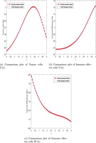
Figure 2. Comparison of compartment of Cancer dynamical model with two numerical method with fractional order $\alpha =0.95$ and m = 256 with time t = 40 days. (a) Time sequence diagram of Tumour cells $U\left(t\right)$. (b) Time sequence diagram of Immune effector cells $V\left(t\right)$ and (c) Time sequence diagram of Immune effector cells $W\left(t\right)$.

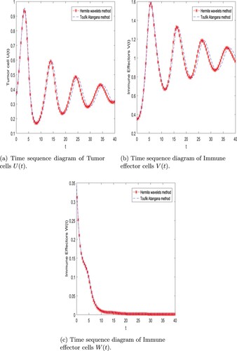
Figure 3. 3D plot of compartment of Cancer dynamical model with Hermite wavelet method with integer order $\alpha =1$ and m = 256. (a) Three-dimensional plot of Tumour cells $U\left(t\right)$. (b) Three-dimensional plot of Immune effector cells $V\left(t\right)$ and (c) Three-dimensional plot of Immune effector cells $W\left(t\right)$.

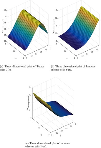
Figure 4. Phase diagram of compartment of Cancer dynamical model with two numerical method with integer order $\alpha =1$ and m = 256 with time t = 5 days. (a) Phase plot of Tumour cells $U\left(t\right)$ and cytotoxic T cells $V\left(t\right)$. (b) Phase plot of cytotoxic T cells $V\left(t\right)$ and natural killer T cells $W\left(t\right)$ and (c) Phase plot of Tumour cells $U\left(t\right)$ and natural killer T cells $W\left(t\right)$.

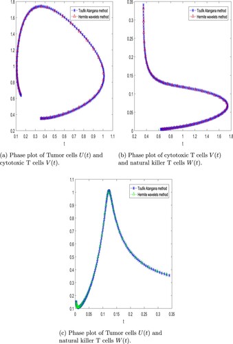
Figure 5. Two-dimensional plot of compartment of Cancer dynamical model with different values of alpha using Hermite wavelet method and m = 256 with time t = 5 days. (a) The graphical behaviour of Tumour cells corresponding to different derivative order α. (b) The graphical behaviour of natural killer T cells corresponding to different derivative order α and (c) The graphical behaviour of cytotoxic T cells corresponding to different derivative order α.

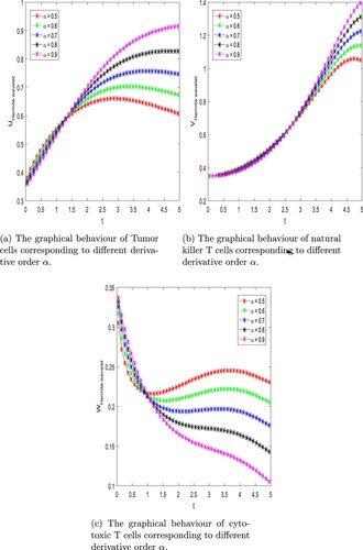
Figure 6. Chaotic phase plot of compartment of Cancer model with Caputo derivative with new numerical scheme with different value of α.

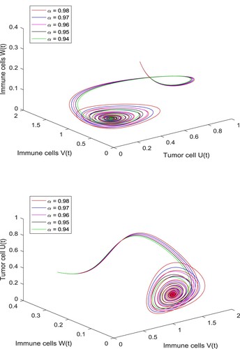
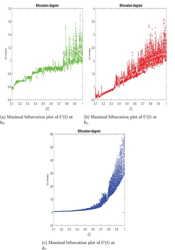
Figure 7. The maximal bifurcation for the Cancer model interpreting Tumour cell $U\left(t\right)$ versus the parameter $k1,d2$ and $d1$. (a) Maximal bifurcation plot of $U\left(t\right)$ at $k_2$. (b) Maximal bifurcation plot of $U\left(t\right)$ at $k_1$ and (c) Maximal bifurcation plot of $U\left(t\right)$ at $d_1$.

6. Some numerical results and discussions

We offer numerical solutions to the cancer model with non-integer order using the Toufik–Atangana method and Hermite wavelet methods in this section. We also show the graphical behaviour of tumour cells and immune effectors for different values of non-integer order α. Further, we assume the non-integer cancer model (1(1) $\begin{array}{rl}{}^C{D}_0^{\alpha }U\left(t\right)& =\mathrm{aU}\left(t\right)-r_{1}U\left(t\right)V\left(t\right)-r_{2}U\left(t\right)W\left(t\right),\\ {}^C{D}_0^{\alpha }V\left(t\right)& =-d_{1}V\left(t\right)+\frac{U^2\left(t\right)V\left(t\right)}{(U^2\left(t\right)+k_1)},\\ {}^C{D}_0^{\alpha }W\left(t\right)& =-d_{2}W\left(t\right)+\frac{U^2\left(t\right)W\left(t\right)}{(U^2\left(t\right)+k_2)},\end{array}$(1) )–(2(2) $(U_0,V_0,W_0)=(0.35,0.35,0.35),$(2) ) with the following parameters values, $\begin{array}{rl}& a\left(t\right)=1,r_1\left(t\right)=1,r_2\left(t\right)=1,d_1\left(t\right)=0.3,d_2\left(t\right)=0.7,\\ & k_1\left(t\right)=0.3,k_2\left(t\right)=0.7,\end{array}$and $(\delta ,\gamma ,\varrho )=(0.35,0.35,0.35).$Numerical simulations and two-dimensional profiles were investigated in this study. Using the proposed numerical method, tumour cells and immune effectors are determined. Figure 1 shows the $2D$ graph of the Tumour cells $U\left(t\right)$, Immune effectors $V\left(t\right)$, and Immune effectors $W\left(t\right)$, obtained via Hermite wavelet and new numerical method with $\alpha =1,m=256$ and also represent the comparison between Hermite wavelet and Toufik-Atangana method. In Figure 1 we can see that the solutions found using the Toufik-Atangana method and Hermite wavelet approaches are identical. Figure 2 shows the $2D$ graph of the Tumour cells $U\left(t\right)$, Immune effectors $V\left(t\right)$, and Immune effectors $W\left(t\right)$, obtained via Hermite wavelet and numerical method with $\alpha =0.95,m=256$ and also represent the comparison between Hermite wavelet and Toufik–Atangana method. The benefit of employing this method lies in its ability to accurately capture the complex dynamics of cancer progression, allowing for more precise modelling and analysis of tumour growth, metastasis, and treatment response. In Figure 2 we can see that the solutions found using the Toufik-Atangana method and Hermite wavelet approaches are identical. Figure 3 shows the $3D$ graph of the Tumour Cells $U\left(t\right)$, Immune effectors $V\left(t\right)$ and Immune effectors $W\left(t\right)$. Figure 4 shows the phase plot of the Tumour cells $U\left(t\right)$ and Immune effectors $V\left(t\right)$ and Immune effectors $W\left(t\right)$ via Toufik-Atangana method and Hermite wavelet method with $\alpha =1,m=256$. Figure 5 shows that 2D profile of Tumour cells $U\left(t\right)$, Immune effectors $V\left(t\right)$, and Immune effectors $W\left(t\right)$ with different values of alpha. Figure 6 represents compartment of Cancer model with 3D phase plot of chaotic behaviour of different values of order of derivative $\alpha =0.98,0.97,0.96,0.95,0.94$. Figure 7 represents maximal bifurcation graph for parameter $k1,k2,d1$ with varies from 0.1 to 1. That maximal bifurcation point, where the system undergoes the most drastic change or exhibits the most complex behaviour. Cancer tumour models often involve systems of differential equations that describe the dynamics of tumour growth, interactions between cancer cells and the micro environment, and the effects of treatment.

Numerical methods, such as Hermite wavelet, finite element, or Toufik Atangana, are used to discretize these equations and solve them numerically over time. This allows researchers to simulate and analyse the behaviour of the cancer model under various conditions (Table 1).

7. Conclusion

The Hermite wavelet approach has been used in this paper to provide numerical solutions for cancer models with nonlinear fractional orders. In addition, stability analysis have explored using the above waveforms. Also we have discussed that the arbitrary order FDEs is an accurate approximation to the Riemann Liouville integration operator. There are many algebraic equations that can be used to solve nonlinear non-integer differential equations using operational matrices and collocation spaces. Another numerical approach, the Taufik–Atangana technique, is briefly explained to demonstrate the accuracy and merit of the proposed technique. The proposed method is defined as stable and iterative. Our graphical simulations showed periodic patterns for various fractional order values with the help of Hermite wavelet method. Hermite wavelet collocation methods are known for their accuracy and precision in solving differential equations. Hermite wavelet methods will provide more computationally efficient solutions than other numerical techniques, especially in problems with high-dimensional parameter spaces. By using fractional order wavelet collocation method in cancer models, we have obtained more accurate and reliable results compared to other numerical techniques.

• In the future, this work will be helpful to solve the IVP of FDEs more accurately and effectively.

• This wavelet collocation method will provide a concise and computationally efficient representation of the underlying dynamics.

• Hermite wavelets is a multi resolution analysis, will allow for a localized representation of solutions.

• This will help the researchers to solve simulations faster and analyse a wider range of scenarios and hypotheses.

Table 1. Comparison between the Tumour cells $U\left(t\right)$ and Immune effectors $V\left(t\right)$, Immune effectors $W\left(t\right)$ using the Hermite wavelet method (HWM) and Toufik-Atangana method $\left(\mathrm{TA}\right)$ for m = 256 and $\alpha =1$.

t	$U_{\mathrm{HWM}}$	$U_{\mathrm{TA}}$	$V_{\mathrm{HWM}}$	$V_{\mathrm{TA}}$	$W_{\mathrm{HWM}}$	$W_{\mathrm{TA}}$
0.1	0.3678	0.3616	0.3501	0.3499	0.3216	0.3305
0.2	0.3809	0.3736	0.3507	0.3502	0.3042	0.3131
0.3	0.3952	0.3867	0.3520	0.3511	0.2881	0.2970
0.4	0.4105	0.4009	0.3539	0.3526	0.2731	0.2820
0.5	0.4271	0.4160	0.3564	0.3546	0.2593	0.2680
0.6	0.4447	0.4323	0.3597	0.3572	0.2464	0.2551
0.7	0.4636	0.4496	0.3637	0.3606	0.2346	0.2431
0.8	0.4835	0.4679	0.3686	0.3646	0.2237	0.2319
0.9	0.5046	0.4873	0.3744	0.3695	0.2136	0.2216

Acknowledgement

Researchers supporting project number-RSPD2024R526, King Saud University, Riyadh, Saudi Arabia.

Disclosure statement

No potential conflict of interest was reported by the author(s).

Data availability statement

Data available on request from the authors.

References

- Mohammadpoor H, Eghbali N, Sajedi L, et al. Stability analysis of fractional order breast cancer model in chemotherapy patients with cardiotoxicity by applying LADM. Adv Contin Discrete Model. 2024;2024(1):6. doi: 10.1186/s13662-024-03800-z
- Sormoli HA, Mojra A, Heidarinejad G. A novel gas embolotherapy using microbubbles electrocoalescence for cancer treatment. Comput Methods Programs Biomed. 2024;244:Article ID 107953. doi: 10.1016/j.cmpb.2023.107953
- Padder A, Almutairi L, Qureshi S, et al. Dynamical analysis of generalized tumor model with Caputo fractional-order derivative. Fractal Fract. 2023;7(3):258. doi: 10.3390/fractalfract7030258
- Butt AR, Saqib AA, Alshomrani AS, et al. Dynamical analysis of a nonlinear fractional cervical cancer epidemic model with the nonstandard finite difference method. Ain Shams Eng J. 2024;15(3):Article ID 102479. doi: 10.1016/j.asej.2023.102479
- Alshammari S, Alshammari M, Alabedalhadi M, et al. Numerical investigation of a fractional model of a tumor-immune surveillance via caputo operator. Alex Eng J. 2024;86:525–536. doi: 10.1016/j.aej.2023.11.026
- Oldham K, Spanier J. The fractional calculus theory and applications of differentiation and integration to arbitrary order. Vol. 111. Elsevier; 1974. ISBN: 9780080956206.
- Kiryakova VS. Generalized fractional calculus and applications. CRC Press; 1993. ISBN: 9780582219779, 0582219779.
- Magin RL. Fractional calculus in bioengineering. Begell House Redding; 2006. doi:10.1615/critrevbiomedeng.v32.i1.10.
- Sabatier J, Agrawal OP, Machado JT. Advances in fractional calculus. Vol. 4. Springer; 2007. ISBN: ISBN-13978-1- 4020-6042-7 (e-book).
- Milici C, Drăgănescu G, Machado JT. Introduction to fractional differential equations. Vol. 25. Springer; 2018. ISBN: 9783030008956, 3030008959 (e-book).
- Kilbas AA, Srivastava HM, Trujillo JJ. Theory and applications of fractional differential equations. Vol. 204. Elsevier Science Limited; 2006. ISBN: 9780444518323 (e-book).
- Kilbas A, Marichev O, Samko S. Fractional integral and derivatives: theory and applications. 1993. ISBN 2-8-8124-864-0 (e-book).
- Yang X-J. General fractional derivatives: theory, methods and applications. Chapman and Hall/CRC; 2019. doi:10.1201/9780429284083.
- Rudolf H. Applications of fractional calculus in physics. World Scientific; 2000. ISBN: 9814496200, 9789814496209 (e-book).
- Podlubny I. Fractional differential equations: an introduction to fractional derivatives, fractional differential equations, to methods of their solution and some of their applications. Vol. 198. Elsevier; 1998. ISBN:9780080531984, 0080531989 (e-book).
- Kumar R, Kumar S, Singh J, et al. A comparative study for fractional chemical kinetics and carbon dioxide CO2 absorbed into phenyl glycidyl ether problems. AIMS Math. 2020;5(4):3201–3222. doi: 10.3934/math.2020206
- Momani S, Kumar R, Srivastava H, et al. A chaos study of fractional sir epidemic model of childhood diseases. Results Phys. 2021;27:Article ID 104422. doi: 10.1016/j.rinp.2021.104422
- Rihan FA. Numerical modeling of fractional-order biological systems. In: Abstract and applied analysis. Vol. 2013. Hindawi; 2013.
- Balcı E, Öztürk İ, Kartal S. Dynamical behaviour of fractional order tumor model with Caputo and conformable fractional derivative. Chaos Solit Fractals. 2019;123:43–51. doi: 10.1016/j.chaos.2019.03.032
- Rihan F, Hashish A, Al-Maskari F, et al. Dynamics of tumor-immune system with fractional-order. J Tumor Res. 2016;2(1):109–115. doi: 10.35248/2684-1258
- Roose T, Chapman SJ, Maini PK. Mathematical models of avascular tumor growth. SIAM Rev. 2007;49(2):179–208. doi: 10.1137/S0036144504446291
- Ahmed E, Hashish A, Rihan F. On fractional order cancer model. J Fract Calc Appl Anal. 2012;3(2):1–6.
- Ghanbari B, Kumar S, Kumar R. A study of behaviour for immune and tumor cells in immunogenetic tumour model with non-singular fractional derivative. Chaos Solit Fractals. 2020;133:Article ID 109619. doi: 10.1016/j.chaos.2020.109619
- Sohail A, Arshad S, Javed S, et al. Numerical analysis of fractional-order tumor model. Int J Biomath. 2015;8(05):Article ID 1550069. doi: 10.1142/S1793524515500692
- Kumar S, Kumar A, Samet B, et al. A chaos study of tumor and effector cells in fractional tumor-immune model for cancer treatment. Chaos Solit Fractals. 2020;141:Article ID 110321.
- Hassani H, Machado J, Avazzadeh Z, et al. Optimal solution of the fractional order breast cancer competition model. Sci Rep. 2021;11(1):1–15. doi: 10.1038/s41598-021-94875-1
- Naik PA, Owolabi KM, Yavuz M, et al. Chaotic dynamics of a fractional order HIV-1 model involving aids-related cancer cells. Chaos Solit Fractals. 2020;140:Article ID 110272. doi: 10.1016/j.chaos.2020.110272
- Zhang L, ur Rahman M, Haidong Q, et al. Fractal-fractional anthroponotic cutaneous leishmania model study in sense of Caputo derivative. Alex Eng J. 2022;61(6):4423–4433. doi: 10.1016/j.aej.2021.10.001
- Zhang L, Rahman MU, Ahmad S, et al. Dynamics of fractional order delay model of coronavirus disease. Aims Math. 2022;7(3):4211–4232. doi: 10.3934/math.2022234
- Fatima B, Rahman MU, Althobaiti S, et al. Analysis of age wise fractional order problems for the covid-19 under non-singular kernel of Mittag–Leffler law. Comput Methods Biomech Biomed Eng. 2023;1–19. doi: 10.1080/10255842.2023.2239976
- Kumar S, Ahmadian A, Kumar R, et al. An efficient numerical method for fractional SIR epidemic model of infectious disease by using Bernstein wavelets. Mathematics. 2020;8(4):558. doi: 10.3390/math8040558
- Shiralashetti S, Kumbinarasaiah S. Hermite wavelets operational matrix of integration for the numerical solution of nonlinear singular initial value problems. Alex Eng J. 2018;57(4):2591–2600. doi: 10.1016/j.aej.2017.07.014
- Agrawal K, Kumar R, Kumar S, et al. Bernoulli wavelet method for non-linear fractional glucose–insulin regulatory dynamical system. Chaos Solit Fractals. 2022;164:Article ID 112632. doi: 10.1016/j.chaos.2022.112632
- Kumar S, Kumar R, Osman M, et al. A wavelet based numerical scheme for fractional order SEIR epidemic of measles by using genocchi polynomials. Numer Methods Partial Differ Equ. 2021;37(2):1250–1268. doi: 10.1002/num.v37.2
- Kumar S, Ghosh S, Kumar R, et al. A fractional model for population dynamics of two interacting species by using spectral and Hermite wavelets methods. Numer Methods Partial Differ Equ. 2021;37(2):1652–1672. doi: 10.1002/num.v37.2
- Saeed U, ur Rehman M. Hermite wavelet method for fractional delay differential equations. J Differ Equ. 2014;2014:Article ID 359093.
- Shiralashetti SC, Srinivasa K. Hermite wavelets method for the numerical solution of linear and nonlinear singular initial and boundary value problems. Comput Methods Differ Equ. 2019;7(2):177–198.
- Kumar S, Kumar R, Cattani C, et al. Chaotic behaviour of fractional predator–prey dynamical system. Chaos Solit Fractals. 2020;135:Article ID 109811. doi: 10.1016/j.chaos.2020.109811
- Toufik M, Atangana A. New numerical approximation of fractional derivative with non-local and non-singular kernel: application to chaotic models. Eur Phys J Plus. 2017;132(10):444. doi: 10.1140/epjp/i2017-11717-0