
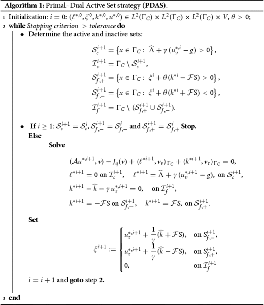
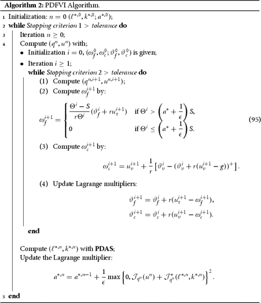
 ?Mathematical formulae have been encoded as MathML and are displayed in this HTML version using MathJax in order to improve their display. Uncheck the box to turn MathJax off. This feature requires Javascript. Click on a formula to zoom.
Abstract
This work deals with a saddle point formulation of parameter identification in linear elastic contact problems with friction. Using the primal–dual formulation of the constrained minimization problem and given observations, we estimate the Lamé coefficients through the penalization and dualization of the considered inverse problem. By Fenchel duality, we provide the dual energy function associated with the constraint. We prove the existence of a solution to the regularized parameter identification problem as well as the convergence of the penalized problem to the original one. An augmented Lagrangian formulation of the inverse problem and the existence of its saddle point are provided. By means of the alternating direction method of multipliers (ADMM) and a primal–dual active set strategy (PDAS), we solve the problem numerically and illustrate our approach.
1. Introduction
The problem of identifying parameters in elliptic boundary value problems from given measurements has a wide range of interesting applications in various fields, such as tomography [Citation1,Citation2], image processing [Citation3,Citation4], groundwater management [Citation5], crack identification [Citation6,Citation7], Lamé coefficients identification [Citation8], and the general framework of optimization problems [Citation9–11]. A general framework for parameter identification in variational, quasivariational, and hemivariational inequalities and their applications can be found in [Citation12–16].
In [Citation17,Citation18], an augmented Lagrangian was formulated for the identification of a discontinuous coefficient, where the state elliptic boundary value problem was reformulated as an equality constraint. Some applications have been devoted to parameter estimation in linear elastic contact problems [Citation8,Citation19,Citation20]. However, accounting for friction complicates the task significantly due to the presence of a non-differentiable term (associated with the considered friction) in the minimization constraint. Thus, standard numerical methods are neither suitable nor applicable. The commonly used approach involves appropriately smoothing the non-smooth term in the variational inequality, reducing it to an equivalent equation; see [Citation21–24] for example. This technique introduces another parameter in addition to the Tikhonov regularization parameter, leading to further complexities. Numerically, although the penalization method is widely used for frictional contact problems, a small penalty parameter choice results in an ill-conditioned system matrix, while a large choice makes the model deviate from its physical meaning.
In the present paper, we explore a saddle point formulation for parameter identification in elastic contact problems with Tresca friction (with a given slip bound). The theoretical and numerical study of contact problems has become extensive, with various methods employed for the numerical analysis and simulation of these complex problems [Citation25–31]. In [Citation32–36], the dual formulation technique based on Fenchel duality theory [Citation37,Citation38] is employed for studying frictional contact problems. The concept involves transforming the non-differentiable problem into a differentiable one subject to inequality constraints.
We examine a case involving a system of an inverse problem, where the equilibrium state is obtained by solving a distributed minimization problem of an energy functional
over the Hilbert space X. This is referred to as the primal problem:
(1)
(1) where we suppose that the energy functional is sum of differentiable and non-differentiable functions. The energy functional depends on an unknown parameter q that belongs to a set
of admissible parameters, which is a subset of a reflexive Banach space (or Hilbert space) Y, i.e.
. Hence, the identification's problem of
from a given measurement
, where the observation operator
lies in
and Z is a Hilbert space of observations, can be approximated by penalizing the classical least square formulation for parameter identification problems given by:
(2)
(2) where
is the solution of the state problem (Equation1
(1)
(1) ) and
is an appropriate norm. Or equivalently, one can write the problem as two levels minimization problem:
(3)
(3) where the abbreviation ‘s.t.’ means ‘subject to’.
Since (Equation1(1)
(1) ) appears in (Equation3
(3)
(3) ) as constraint, solving (Equation1
(1)
(1) ) in first step when the parameter q is still far from its optimal value may be inefficient. Also, one has to make a choice of initialization
and this gives a first approximation of state
which may be far from the measurement [Citation39]. The idea is to compute the dual problem associated to the primal problem (Equation1
(1)
(1) ) using the Fenchel duality:
(4)
(4) where X and
are placed in topological duality and
is the convex conjugate function associated to J. It is well known that the solution to the primal problem (Equation1
(1)
(1) ) and dual problem (Equation4
(4)
(4) ) -if they exist- satisfy the following extremality condition:
(5)
(5) where
is the solution of (Equation1
(1)
(1) ) and
is the solutions of (Equation4
(4)
(4) ) (see [Citation37] for more details). One can take profit from this relation to get a penalization of the least square problem (Equation3
(3)
(3) ) (see [Citation39]). Then, the penalized least square formulation (see [Citation40]) for parameter identification problem is stated as follows:
(6)
(6) Once the existence of a solution and the convergences are obtained, by keeping the extremality duality inequality relation as constraint (since weak duality
is always satisfied), we get the following constrained minimization problem
(7)
(7) We state the augmented Lagrangian functional associated with (Equation7
(7)
(7) ), where the quadratic term
is added to the Lagrangian function. Then, we reformulate the inverse problem as an equivalent saddle point problem. We utilize an ADMM (Alternating Direction Method of Multipliers) to split the problem into several subproblems. Additionally, we employ Fenchel duality and a primal–dual active set strategy (PDAS) to numerically solve the resulting subproblems.
The remainder of this paper is briefly outlined as follows. In Section 2, we formulate the identification problem. Firstly, we reformulate the frictional contact problem as an equivalent minimization problem and compute the associated regularized dual problem. Secondly, we formulate the regularized penalized problem as the least squares identification of Lamé coefficients. We establish the existence of a solution based on a minimizing sequence and demonstrate the convergence of the regularized penalized least squares problem to the original regularized least squares problem based on Sobolev embeddings. In Section 3, we introduce the Lagrangian and augmented Lagrangian formulations of the inverse problem. We demonstrate the existence of Lagrange multipliers. Finally, we provide an equivalent saddle point. Section 4 is devoted to the numerical realization of the problem. We present the algorithms and illustrate the solutions
2. Penalized identification problem formulation
2.1. Elastic contact problem with friction
We are interested in an elastic body occupying in its initial ( non-deformed) configuration a bounded domain , with a smooth boundary
. We assume that Γ is divided into three disjoint parts, i.e.
and
. We assume that the body is clamped on
and a surface traction is applied on
. On
the body may come into a frictional contact with a rigid foundation. We assume a linear elasticity, then the strain tensor ε is given by:
where u is the displacement field.
The constitutive relation is:
where
is the (fourth-order) symmetric and coercive elasticity tensor. Let ν be the unit outward normal to Ω on Γ. The displacement field and the stress tensor can be decomposed in normal and tangential components as follows:
The mechanical equilibrium equation is given by:
(8)
(8)
(9)
(9)
(10)
(10) where
and
.
Let be the gap between Ω and the rigid foundation. The unilateral contact conditions are then:
(11)
(11) The Coulomb friction is given by:
(12)
(12) The Tresca friction is given by:
(13)
(13) where
is the friction coefficient.
There are a major mathematical difficulties inherent in the problem (Equation8(8)
(8) )–(Equation12
(12)
(12) ). For instance, in general,
in (Equation13
(13)
(13) ) is neither pointwise nor almost everywhere defined. Replacing the Coulomb friction in the above model by Tresca friction means replacing
by a given friction
. The resulting system can be then analysed and the existence of a unique solution can be proved. For a review, we refer the reader to [Citation26,Citation41], for example. In the remainder of this work, we will consider the Tresca friction (Equation13
(13)
(13) ) since the problem with (Equation12
(12)
(12) ) can be obtained by a sequence of problems with the Tresca friction (Equation13
(13)
(13) ) (see [Citation41] for example).
In the following, we introduce the notations and recall some necessary definitions that we will need later. We denote by the usual Sobolev space and
are real Hilbert spaces endowed with the inner products:
under summation convention, and
The associated norms are
,
,
,
and
, respectively. And we recall the following Rellich Kondrachov compactness theorem [Citation42]:
Theorem 2.1
Assume that Ω is a bounded open subset of , and
is
. Suppose
, then:
(14)
(14) for each
. In particular, when p = d, we have
(15)
(15) for
.
Keeping in mind the boundary conditions (Equation11(11)
(11) )–(Equation13
(13)
(13) ), we introduce the closed subspace V of
and K the set of admissible displacements defined respectively by:
Define the following set:
The Hilbert space V is endowed with the inner product given by:
(16)
(16) By Korn's inequality, there exists a constant
such that:
(17)
(17) Note that by the Korn's inequality, the norm
and the usual norm of
are equivalent (see [Citation28] for example).
We use the Riesz's representation theorem to consider the element by:
(18)
(18) We define the mapping
by:
(19)
(19) With the above notations, we obtain the following variational formulation of the problem (P):
Problem (PV ). Find a displacement field such that:
(20)
(20) The existence of the solution of the problem (PV ) is widely studied [Citation25–31] and the uniqueness depends on the smallness of the friction's coefficient
, where
on
(see [Citation41]).
Now, we are able to give an equivalent minimization problem. To do this, let us introduce the following notations:
(21)
(21)
(22)
(22)
(23)
(23) And the linear maps A and B are defined respectively by:
Hence, the problem (Equation20
(20)
(20) ) is equivalent to the following minimization problem, known as primal problem:
Primal Problem:
(24)
(24) where
. Since the symmetric and bilinear form
is coercive,
is linear and continuous and
is strictly convex and lower semicontinuous, the minimization problem (Equation24
(24)
(24) ) admits a unique solution (see [Citation37]).
Now, we give the dual problem associated to (Equation24(24)
(24) ) taking into account the separability of cost function into sum of three proper, convex and lower semi continuous functions. For the convex conjugate
of
, one derives that
equals
unless
(25)
(25) Note that in that in (Equation25
(25)
(25) ), the regularity
for
is the best that we can suppose to allow the convergence (see [Citation43,Citation44]).
Further, one obtains
(26)
(26) and
(27)
(27) Since
, we have:
(28)
(28) Then, the dual problem is defined as follows:
(29)
(29) Evaluating the extremality conditions for the above problems, we obtain the following lemma [Citation36,Citation45]:
Lemma 2.2
The solution of the primal problem (Equation24
(24)
(24) ) and the solution
are related by
and the existence of
such that:
(30)
(30)
(31)
(31)
(32)
(32)
(33)
(33) for an arbitrary
.
Following [Citation36,Citation45], we introduce regularized version of the contact problem with Tresca friction, which enable us to apply the semismooth Newton method. To this end, let be a regularization parameter,
,
and
. Let us define the functional
by:
(34)
(34) where
satisfies:
(35)
(35) Then, the regularized dual problem with Tresca friction is defined as:
(36)
(36) It can be proved (see [Citation36,Citation45]) that the extrimality conditions relating the primal and the regularized dual problem are, for
:
(37)
(37)
(38)
(38)
(39)
(39) for any
. Here, ξ is the Lagrange multiplier associated to the constraint
.
2.2. Primal–dual parameter estimation problem
We are interested in a simple situation of an isotropic elasticity where the elasticity tensor depends only on two independent moduli. For instance,
can be expressed in terms of the Lamé coefficients
by:
(40)
(40) Other commonly used elastic parameters are the Young modulus E and the Poisson ratio ν, which are related to the Lamé constants by:
(41)
(41) The following inequality, which holds pointwise in Ω for d = 2, is easy to establish:
(42)
(42) From (Equation17
(17)
(17) ) and (Equation42
(42)
(42) ), one can obtain:
(43)
(43) where
. For given positive constants
and
satisfying
, we define the following subset of
of elements of the form
:
Henceforth, we will assume that a (possibly noisy) measurement z of
is available, where
and
together satisfy (Equation24
(24)
(24) ). The purpose of this paper is to propose and analyse a method for estimating q from z. For this reason, a least squares formulation associated to the estimation of the Lamé parameters
is considered:
(44)
(44) where
is the unique solution of (Equation24
(24)
(24) ) corresponding to q.
In principle, it is reasonable to estimate q by minimization problem (Equation44(44)
(44) ) over
. However, since the inverse problem under consideration is ill-posed, it is necessary to regularize the cost function.
Therefore, we consider the following minimization regularized problem to estimate q from z. Find by solving:
(45)
(45) where R is a Tikhonov regularization and
is the Tikhonov's regularization parameter.
Now, we are in position to state the primal–dual formulation for least squares parameter estimation problem:
(46)
(46)
2.3. Convergence results
The first result in this section confirms the existence of at least one solution to the primal–dual problem (Equation46(46)
(46) ).
Proposition 2.1
For every , there exists a solution
to (Equation46
(46)
(46) ).
Proof.
Let be a minimizing sequence such that for each
the constraints in (Equation46
(46)
(46) ) are fulfilled, that is:
(47)
(47) and
(48)
(48) here α denotes the infimum of the cost function in (Equation46
(46)
(46) ). Since
is not negative and
is coercive and from (Equation48
(48)
(48) ), the sequence
is bounded. Hence, there exists a subsequence of
, which is denoted by the same notation
, and
such that
(49)
(49) In particular, since
, we get
(50)
(50) Moreover
(51)
(51) also, it follows that
(52)
(52) and then
(53)
(53) In the other hand, we have:
(54)
(54) Let us prove the following continuity result:
(55)
(55) Since
and
both satisfy the variational formulation (Equation20
(20)
(20) ) for
and
, respectively, i.e.
(56)
(56) and
(57)
(57) Taking
in (Equation56
(56)
(56) ) and
in (Equation57
(57)
(57) ), by adding the resulting inequality, we obtain:
(58)
(58) Let us set for the sake of simplicity:
this leads to
(59)
(59) which is equivalent to
(60)
(60) Now, taking v = 0 in (Equation20
(20)
(20) ) we deduce the existence of positive constant C, C will be generating constant in the remainder of the paper, such that
(61)
(61) and since
and u are bounded, there exists a constant C such that
(62)
(62) Also, we have
(63)
(63) From the coercivity of
and from (Equation60
(60)
(60) ), there exists a positive constant C such that
(64)
(64) Since
converges weakly in
which is compactly embedded in
, then
converges strongly in
and the right side in (Equation64
(64)
(64) ) tends to zero.
From (Equation52(52)
(52) ), (Equation53
(53)
(53) ) and (Equation64
(64)
(64) ) we conclude the existence of a solution to (Equation46
(46)
(46) ).
In this subsection, we turn to the convergence of the sequence to a solution of (Equation45
(45)
(45) ).
Proposition 2.2
For every , let
denote a solution to (Equation46
(46)
(46) ). Then
contains a weakly convergent subsequence as
and every weak cluster point
is a solution to (Equation45
(45)
(45) ).
Proof.
Let be such that
satisfies the constraints in (Equation46
(46)
(46) ). Then,
and for every
we have:
(65)
(65) Since
and
, then,
(66)
(66) and hence
is bounded in
. It follows that there exists a subsequence of
, denoted by
, weakly convergent in
to
.
As in the proof of Proposition 2.1, taking the limit as in (Equation66
(66)
(66) ) we obtain:
(67)
(67) and then, we get
(68)
(68) which implies that
satisfies all constraints in the problem (Equation46
(46)
(46) ). Furthermore, by (Equation65
(65)
(65) ) we have
(69)
(69) for all
such that there exists
with
is admissible for (Equation46
(46)
(46) ). It follows that
is a solution to (Equation45
(45)
(45) ).
3. Augmented Lagrangian formulation
In this section, we provide a new inverse problem formulation. Since the relation formulation between the primal and dual problems is given by:
(70)
(70) where
is the solution of the primal problem and
is the solution of the dual problem.
Hence, to provide the Lagrangian formulation of the inverse problem, we retain the above equation as a constraint in (Equation46(46)
(46) ). Thus, we consider the following constrained problem:
(71)
(71) By the weak duality, one have:
then, we can replace the equality constraint by the remaining inequality, thus:
(72)
(72) The Lagrangian formulation of (Equation72
(72)
(72) ) is as follows:
(73)
(73) where
is the Lagrange multiplier,
and
In the next, we give a result providing the existence of Lagrange multiplier
.
Theorem 3.1
is a solution of (Equation45
(45)
(45) ) if and only if there exists
such that
is a saddle point of the augmented Lagrangian
, i.e.
(74)
(74)
Proof.
Let be a closed convex cone in
defining the natural partial ordering relation
, the dual cone
and
its polar cone. The following properties are straightforward:
The map
is convex with respect to
For each
The set
The constraint qualification hypothesis (Slater condition):
Then, the primal problem (Equation45(45)
(45) ) stable. Now, following [Citation37], we will consider the problem (Equation45
(45)
(45) ) as a primal problem and we are looking to define its dual problem using a family of perturbed problems, where the perturbed costs are defined by:
The dual problem is hence defined by:
which is equivalent to
(75)
(75) Since
as
with 1)-4), then the primal problem and dual problem have at least one solution
and
, respectively, which satisfy the strong duality. And we have the extrimality condition:
(76)
(76) The proof is achieved with application of [Citation37, Theorem 5.1].
We are interested in the augmented Lagrangian formulation of the inverse problem. Utilizing the dualization and penalization technique, we define the Lagrangian functional for the following penalized constrained problem:
(77)
(77) Then the augmented Lagrangian formulation of (Equation77
(77)
(77) ) is as follows:
(78)
(78) where
is the Lagrange multiplier.
Finally, the constrained minimization problem (Equation77(77)
(77) ) is equivalent to the following saddle point problem:
(79)
(79) And it is well known that
is saddle point for
if and only if it is a saddle point for
.
4. Algorithms and numerical examples
This section is devoted to the numerical treatment and realization of Lamé coefficients identification. The saddle point problem is obtained, we proceed by an ADMM to split the problem and we apply different numerical methods as intern solvers.
4.1. Algorithms
We develop a splitting algorithm for the numerical solution to the problem defined by (Equation46(46)
(46) ). The splitting algorithm is an ADMM based on an augmented Lagrangian formulation for inequality constraints [Citation46].
The ADMM in Gauss Seidel fashion is stated as follows:
Starting with initial guess , for
compute:
(80)
(80)
(81)
(81) Update the Lagrange multiplier as follows:
(82)
(82) The subproblem (Equation80
(80)
(80) ) is equivalent to a non-smooth minimization problem, with respect to
over
, whose cost function is the following map:
after neglecting the constant terms.
The non-smoothness of this minimization problem come originally from the terms associated to the friction in the cost function of the state unknown. Furthermore, we need to deal with the contact condition, i.e. the constraint in the admissible subset K. To overcome all of the cited complexities, we iterate the use of the ADMM for splitting the contact and friction.
To do this, let us introduce three auxiliary unknowns to decouple the linear elasticity from contact and friction in (Equation80(80)
(80) ). Firstly, let us introduce the following subset
The problem (Equation80
(80)
(80) ) becomes:
(83)
(83) By setting
Then, the Lagrangian functional associated to the constrained minimization problem (Equation83
(83)
(83) ) is then, for
,
The ADMM that is employed, is stated as follows:
Starting with an initial guess ;
Compute in Gauss-Seidel fashion the following sub-problems: (84)
(84)
(85)
(85)
(86)
(86) Update the Lagrange multipliers:
(87)
(87)
(88)
(88) The sub-problem (Equation84
(84)
(84) ) is equivalent to minimization problem:
(89)
(89) where the cost function, after neglecting the constant terms, is as follows:
which is Gâteaux differentiable.
The sub-problem (Equation85(85)
(85) ) is equivalent to the minimization problem
(90)
(90) In order to get the solution of this problem, one can use the Fenchel duality. Following [Citation37], the solution can be explicitly computed, and it is given by:
(91)
(91) And the sub-problem (Equation86
(86)
(86) ) is equivalent to the following minimization problem:
(92)
(92) The solution to the above minimization problem can be explicitly computed by employing KKT condition, and it is given as follows:
(93)
(93) where
. Therefore, the auxiliary unknowns
and
are computed with a negligible cost.
Now, we turn to the sub-problem (Equation81(81)
(81) ). This problem is equivalent to a minimization problem for which the cost function, after neglecting the constant terms, is given by
(94)
(94) In practice, the minimization problem (Equation94
(94)
(94) ) corresponds exactly to the dual problem (Equation29
(29)
(29) ) multiplied by
. This problem involves an inequality-constrained minimization of a quadratic functional, whereas the primal problem deals with a non-differentiable functional. Therefore, solving (Equation94
(94)
(94) ) is equivalent to solving (Equation37
(37)
(37) )–(Equation39
(39)
(39) ). We can utilize a Primal–Dual Active Set Strategy algorithm (PDAS) for this purpose (see [Citation35,Citation36,Citation45]).
Since and
. Then, the variational equation in PDAS algorithm is equivalent to the following equation:
which is clearly equivalent to:
where
if
and
otherwise.
In the Algorithm 2, we presume the solutions of the subproblems (Equation80(80)
(80) )–(Equation82
(82)
(82) ).
4.2. Finite element discretization
The aim of this section is to present a computer implementation of the proposed theoretical approach and numerical scheme through representative numerical example. For the sake of simplicity, we treat a two-dimensional simple example i.e. we suppose that is polygonal domain. Let
be the space of continuous and piecewise affine functions, i.e.
where
is a family of polygons forming Ω (mostly triangles) and
is the space of polynomials of global degree is less or equal to one in T (see [Citation47]). Vectorized Matlab codes for linear two-dimensional elasticity [Citation48] are used to the assembly of the matrices associated to the operators in the algorithms.
Let be the system of piecewise global basis functions of
. For
, we have:
(96)
(96) We employ Voigt's representation of the linear strain tensor as in [Citation48,Citation49], on one hand we have:
(97)
(97) and then, the elastic constitutive equation is given by:
(98)
(98) where
Then, we can write
On the other hand, let
be the transpose of the vector of nodal values of
on a triangle
. We have:
(99)
(99) where
denotes the derivative with respect to ‘·’ and
is the area of the triangle T. Then, we can get the matrix associated to strain deformation defined by:
(100)
(100) Then, one may write, for
and
,
and
4.3. Example
As example, we consider the problem in linear elasticity (under the hypothesis of small deformations). The domain is discretized using Matlab mesh generator developed in [Citation50]. In Figure , we visualize the domain.
Figure 1. The initial configuration.
To compute the observation, we use the following material constants:
The observed Lamé coefficients are:
The body is clamped from
The load force is
The gap between the foundation and the contact zone
All parameters in the above algorithms are chosen like:
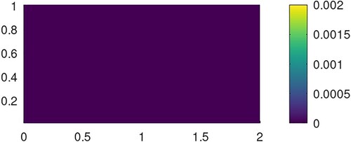
Figure 2. The observed state and its von Mises distribution.
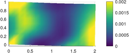
Figure 3. The estimated state and its von Mises distribution.
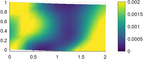
Table 1. The errors between the observations and the estimations.
Table 2. The errors between the observations with noise and the estimations.
5. Conclusion
In this paper, we have investigated a primal dual formulation of parameter identification in elastic contact problem with given friction. This approach allows us to reformulate the constrained problem as saddle point problem which will be more useful for the numerical realization of this problem. We have provided a saddle point formulation for the considered inverse problem, the second step was the numerical realization of this problem. This work may be considered as a framework for inverse problems in linear elasticity. Further coming works will be concerned in the employment of this approach for identification of other parameters in frictional contact problem. Considering a regularity weaker than in admissible set
will be an important perspective as well as an inverse problem subject to hemi-variational inequalities. Identifying Lamé coefficients for contact problem with elastic-locking or hyperelastic and elastoplastic materials will be an important issue in future works. Nevertheless, there are some important issues to address in order to overcome the limitations of the proposed study:
An active set strategy method have been used to solve the dual problem. Compared to others methods, it is well known that this method is very slow since the active and inactive sets are updated during the iterations.
Research alternative function spaces that offer weaker regularity conditions while still providing sufficient structure for solving the problem at hand. For example, Sobolev spaces of lower regularity such as
Financial interests
Authors declare they have no financial interests.
Acknowledgments
The authors of this paper express their heartfelt gratitude to the Editorial Office, Editor-in-Chief, Associate Editors, and anonymous reviewers for their valuable and constructive comments and remarks. Their insightful feedback greatly contributed to enhancing the quality and clarity of this work.
Data availability
Data sharing not applicable to this article as no datasets were generated or analysed during the current study.
Disclosure statement
No potential conflict of interest was reported by the author(s).
Additional information
Funding
References
- Goncharsky AV, Romanov SY. Iterative methods for solving coefficient inverse problems of wave tomography in models with attenuation. Inverse Probl. 2017;33(2):Article ID 025003. doi: 10.1088/1361-6420/33/2/025003
- Li F, Abascal JF, Desco M, et al. Total variation regularization with split Bregman-based method in magnetic induction tomography using experimental data. IEEE Sens J. 2016;17(4):976–985. doi: 10.1109/JSEN.2016.2637411
- Chen M, Zhang H, Lin G, et al. A new local and nonlocal total variation regularization model for image denoising. Cluster Comput. 2019;22(S3):7611–7627. doi: 10.1007/s10586-018-2338-1
- Zhang D, Shi K, Guo Z, et al. A class of elliptic systems with discontinuous variable exponents and L1 data for image denoising. Nonlinear Anal Real World Appl. 2019;50:448–468. doi: 10.1016/j.nonrwa.2019.05.012
- Ayvaz MT. A hybrid simulation–optimization approach for solving the areal groundwater pollution source identification problems. J Hydrol. 2016;538:161–176. doi: 10.1016/j.jhydrol.2016.04.008
- Abda AB, Ameur HB, Jaoua M. Identification of 2D cracks by elastic boundary measurements. Inverse Probl. 1999;15(1):67–77. doi: 10.1088/0266-5611/15/1/011
- Bodart O, Cayol V, Dabaghi F, et al. Fictitious domain method for an inverse problem in volcanoes. In: International Conference on Domain Decomposition Methods. Cham: Springer; 2018. p. 409–416.
- Jadamba B, Khan AA, Raciti F. On the inverse problem of identifying Lamé coefficients in linear elasticity. Comput Math Appl. 2008;56(2):431–443. doi: 10.1016/j.camwa.2007.12.016
- Banks HT, Kunisch K. Estimation techniques for distributed parameter systems. Birkhäuser Boston: Springer Science & Business Media; 2012.
- Engl HW, Hanke M, Neubauer A. Regularization of inverse problems. Birkhäuser Boston: Springer Science & Business Media; 1996.
- Sofonea M, Xiao YB, Couderc M. Optimization problems for a viscoelastic frictional contact problem with unilateral constraints. Nonlinear Anal Real World Appl. 2019;50:86–103. doi: 10.1016/j.nonrwa.2019.04.005
- Gwinner J, Jadamba B, Khan AA, et al. Identification in variational and quasi-variational inequalities. J Convex Anal. 2018;25(2):545–569.
- Hao DN, Khan AA, Sama M, et al. Inverse problems in variational inequalities by minimizing energy. Pure Appl Funct Anal. 2019;4(2):247–269.
- Khan AA, Motreanu D. Inverse problems for quasi-variational inequalities. J Glob Optim. 2018;70(2):401–411. doi: 10.1007/s10898-017-0597-7
- Migórski S. Parameter identification for evolution hemivariational inequalities and applications. In: Inverse problems in engineering mechanics III. Elsevier Science Ltd; 2002. p. 211–218.
- Migórski S, Khan AA, Zeng S. Inverse problems for nonlinear quasi-variational inequalities with an application to implicit obstacle problems of p-Laplacian type. Inverse Probl. 2019;35(3):Article ID 035004.
- Chen Z, Zou J. An augmented lagrangian method for identifying discontinuous parameters in elliptic systems. SIAM J Control Optim. 1999;37(3):892–910. doi: 10.1137/S0363012997318602
- Gockenbach MS, Khan AA. An abstract framework for elliptic inverse problems: part 2. an augmented lagrangian approach. Math Mech Solids. 2009;14(6):517–539. doi: 10.1177/1081286507087150
- Bonnet M, Constantinescu A. Inverse problems in elasticity. Inverse Probl. 2005;21(2):R1–R50. doi: 10.1088/0266-5611/21/2/R01
- Gockenbach MS, Khan AA. An abstract framework for elliptic inverse problems: part 1. an output least-squares approach. Math Mech Solids. 2007;12(3):259–276. doi: 10.1177/1081286505055758
- Amassad A, Chenais D, Fabre C. Optimal control of an elastic contact problem involving Tresca friction law. Nonlinear Anal. 2002;48(8):1107–1135. doi: 10.1016/S0362-546X(00)00241-8
- Capatina A. Optimal control of a signorini contact problem. Numer Funct Anal Optim. 2000;21(7-8):817–828. doi: 10.1080/01630560008816987
- Essoufi EH, Zafrar A. Optimal control of friction coefficient in signorini contact problems. Optim Control Appl Methods. 2021;42(6):1794–1811. doi: 10.1002/oca.v42.6
- Matei A, Micu S. Boundary optimal control for nonlinear antiplane problems. Nonlinear Anal Theory Methods Appl. 2011;74(5):1641–1652. doi: 10.1016/j.na.2010.10.034
- Andersson T. The boundary element method applied to two-dimensional contact problems with friction. In: Boundary element methods. Berlin: Springer; 1981. p. 239–258.
- Capatina A. Variational inequalities and frictional contact problems. New York: Springer; 2014.
- Ciulcu C, Motreanu D, Sofonea M. Analysis of an elastic contact problem with slip dependent coefficient of friction. Math Inequal Appl. 2001;4:465–479.
- Duvant G, Lions JL. Inequalities in mechanics and physics. Birkhäuser Boston: Springer Science & Business Media; 2012.
- Haslinger J, Kučera R, Riton J, et al. A domain decomposition method for two-body contact problems with Tresca friction. Adv Comput Math. 2014;40(1):65–90. doi: 10.1007/s10444-013-9299-y
- Kikuchi N, Oden JT. Contact problems in elasticity: a study of variational enequalities and finite element methods. Philadelphia: Society for Industrial and Applied Mathematics; 1988.
- Sofonea M, Matei A. Variational inequalities with applications: a study of antiplane frictional contact problems. Birkhäuser Boston: Springer Science & Business Media; 2009.
- Essoufi EH, Koko J, Zafrar A. Alternating direction method of multiplier for a unilateral contact problem in electro-elastostatics. Comput Math Appl. 2017;73(8):1789–1802. doi: 10.1016/j.camwa.2017.02.027
- Essoufi EH, Zafrar A. Dual methods for frictional contact problem with electroelastic-locking materials. Optimization. 2021;70(7):1581–1608. doi: 10.1080/02331934.2020.1745794
- Hüeber S, Stadler G, Wohlmuth BI. A primal–dual active set algorithm for three-dimensional contact problems with coulomb friction. SIAM J Sci Comput. 2008;30(2):572–596. doi: 10.1137/060671061
- Kunisch K, Stadler G. Generalized Newton methods for the 2D-signorini contact problem with friction in function space. ESAIM: Math Model Numer Anal. 2005;39(4):827–854. doi: 10.1051/m2an:2005036
- Stadler G. Semismooth Newton and augmented lagrangian methods for a simplified friction problem. SIAM J Optim. 2004;15(1):39–62. doi: 10.1137/S1052623403420833
- Ekeland I, Temam R. Convex analysis and variational problems. Philadelphia: Society for Industrial and Applied Mathematics; 1999.
- Rockafellar RT. Convex analysis. Vol. 18. Princeton: Princeton University Press; 1970.
- Chavent G, Kunisch K, Roberts JE. Primal–dual formulations for parameter estimation problems. Comput Appl Math. 1999;18:173–229.
- Bertsekas DP. Constrained optimization and lagrange multiplier methods. Academic Press; 2014.
- Dostál Z, Haslinger J, Kučera R. Implementation of the fixed point method in contact problems with coulomb friction based on a dual splitting type technique. J Comput Appl Math. 2002;140(1-2):245–256. doi: 10.1016/S0377-0427(01)00405-8
- Evans LC. Partial differential equations. Vol. 19. American Mathematical Soc; 2010.
- Daras NJ, Rassias TM, editors. Operations research, engineering, and cyber security: trends in applied mathematics and technology. Springer; 2017.
- Dreves A, Gwinner J, Ovcharova N. On the use of elliptic regularity theory for the numerical solution of variational problems. In: Operations research, engineering, and cyber security. Cham: Springer; 2017. p. 231–257.
- Ito K, Kunisch K. Lagrange multiplier approach to variational problems and applications. Philadelphia: Society for Industrial and Applied Mathematics; 2008.
- Giesen J, Laue S. Combining ADMM and the augmented Lagrangian method for efficiently handling many constraints. In: IJCAI; 2019. p. 4525–4531.
- Ciarlet PG. The finite element method for elliptic problems. Philadelphia: Society for Industrial and Applied Mathematics; 2002.
- Koko J. Vectorized matlab codes for linear two-dimensional elasticity. Sci Program. 2007;15(3):157–172.
- Alberty J, Carstensen C, Funken SA, et al. Matlab implementation of the finite element method in elasticity. Computing. 2002;69(3):239–263. doi: 10.1007/s00607-002-1459-8
- Koko J. A matlab mesh generator for the two-dimensional finite element method. Appl Math Comput. 2015;250:650–664. doi: 10.1016/j.amc.2014.11.009