Generation of fractal curves using new binary 8-point interpolatory subdivision scheme

Abstract

The subdivision scheme is a valuable tool for designing shapes and representing geometry in computer-aided geometric design. It has excellent geometric properties, such as fractals and adjustable shape. In this research paper, we explore the generation of fractal curves using a novel binary 8-point interpolatory subdivision scheme with two parameters. We analyse different properties of the proposed scheme, including convergence, special cases, and fractals. Additionally, we demonstrate through various examples the relationship between the shape parameters and the fractal behaviour of the resulting curve. Our research also identifies a specific range of shape parameters that can effectively produce fractal curves. The findings of this study provide a fast and efficient method for generating fractals, as demonstrated by numerous examples. Modelling examples show that the 8-point interpolatory scheme can enhance the efficiency of computer design for complex models.

Keywords:

• Interpolatory subdivision scheme
• binary 8-point scheme
• continuity
• generation of fractal curves
• fractal properties

2020 Mathematics Subject Classifications:

• 43-08
• 43-11
• 39-00
• 39-03
• 39-11

1. Introduction

Subdivision is a well-organized technique for producing curves and surfaces in Computer Aided Geometric Design (CAGD). The subdivision technique is mathematical by its nature thus very simple to implement on computer systems and consequently has a wide range of applications in various industries. Some examples are animation i.e film making, aircrafts i.e ship making, utensils making, furniture industry, machinery production, the vehicles industry and jewelry making. In general, subdivision schemes can be divided into two categories: Interpolatory schemes and Approximating schemes. Interpolatory schemes get better shape control while approximating schemes have better smoothness. The interpolating subdivisions schemes are more gorgeous then approximating schemes because of their interpolating property.

The history of subdivision schemes started when the first subdivision scheme was presented by Rham [1]. This scheme was a recursive corner-cutting piecewise linear approximation to generate $C^1$- continuous smooth curves, which opened new dimensions in the field of geometric modelling. Ko et al. [2] reconstructed the mask of interpolating symmetric subdivision systems, $2n$-point binary interpolating systems and the 4-point ternary interpolating scheme by using the essential condition for smoothness and symmetry. Rehan and Sabri [3] introduced a combined ternary four-point subdivision scheme. Laurent polynomial method is used to evaluate the continuity and observed that this scheme generates interpolating $C^1$ and approximating $C^1$, $C^2$, $C^3$ limiting curves. Ghaffar et al [4] introduced a new non-stationary $2m$-point subdivision scheme that satisfies some of the mentioned properties are curvature, torsion monotonicity shape preservation and continuity. Ghaffar et al [5] introduced the non-stationary binary $(2s-1)$-point subdivision schemes for integer $\ge 2$. The Lagrange polynomial method is used to establish the schemes that reproduce polynomial degree $(2s-2)$. The importance of these schemes is proved with the help of different examples.

In last few decades, computational geometry by using SSs have attained much attention. Mustafa et al. [6–8] devised parametric schemes using a new type of Lagrange polynomial that employs a single shape parameter. Ghaffar et al. [9–12] created continuity conditions to represent complex, free-form unified Shape Splines (SSs) with one shape control parameter. These methods allow for the creation of intricate shapes through the use of shape control unified SSs. These approaches inherit the strengths of non-parametric SSs and resolve the issue of shape control in SSs by employing tension control shape parameters. The proposed methods use varied techniques to construct composite curves with higher smoothness conditions, using simple and straightforward computations with linear polynomials instead of trigonometric functions. In 2020, Ashraf et al. [13–15] introduced a new method for generalizing SSs with a single shape parameter. Shahzad et al. [16] developed a numerical algorithm to calculate the subdivision depth of binary SSs with shape parameters.

Hussain et al. [17] proposed a subdivision algorithm with varying arity that explores properties such as continuity, regularity, error bound, and limit curve shape. Ashraf et al. [18, 19] presented a generalized algorithm to develop a class of approximating binary subdivision schemes. Mustafa et al. [20] introduced a numerical approach for solving second-order singularly perturbed boundary value problems. Bari et al. [21] unified the interpolating nonstationary subdivision scheme with a tension control parameter to construct a link between nonstationary SSs and applied geometry.

Fractals are the patterns that are infinitely complex patterns. These are made up by repeatedly using a basic operation in an ongoing feedback iterative process. Nature is filled with hundreds of fractals varieties. Trees and their leaves, mountains ranges, systems of rivers, snowflakes, crystals, sea-shells, sea-stars, clouds, lighting, fruits like pineapple, vegetables like cauliflower or broccoli, blood vessels, and many other examples like these exhibit formation of fractals. The self-similarity of fractals makes it an attractive factor for creative work. From paintings, sculptures, textiles to graphic designing, animations and in every domain of artistic work is affected by fractals.

Doo and Sabin [22] discussed the functioning of the limits surface using eigenvalues of a set of matrices, defined by a recursive division construction. Carpenter [23], generated fractal curves and surfaces by using a simple set of methods and presented the idea of the statistical subdivision. Mandelbrot [24] shed light on fractals that exists in nature's beauty and devised fractal geometry that studied self-similar and irregular geometric shapes and has an in-depth presentation at arbitrarily small scales. Soon after that, several procedures had started to formulate to create fractals. Bouboulis and Dalla [25] derived the fractal interpolation surfaces from its respective functions and proved some interesting properties of them. Zheng et al. [26] used a new mechanism to evaluates the fractal characteristics of binary four point and ternary three point interpolating subdivision schemes. Later on a relationship is found between shape parameter and fractal behaviour of the boundary curves of the both schemes respectively. The production of fractal curves and surfaces are also discussed. The three point ternary interpolating scheme with two shape parameters that was devised by Hassan is examined by Zheng et al. [27].

Many examples are elaborated by author that demonstrates the true direction for creation of fractal curves and surfaces. By using this method fractal range of this scheme is also obtained. Mustafa et al. [28] discussed the engineering images by the fractal proprieties of binary 6-point interpolating scheme. A relationship between the fractal dimension of the fractal limit curve and shape parameter is also found and show that this scheme is best for the modelling of fractal antennas, garari's, bearing and rock etc. Peng et al. [29] have conducted a study on the fractal properties of a ternary 4-point rational interpolation SS. Meanwhile, Bari et al. [30] have proposed a method for constructing fractal curves using a 7-point binary approximating SS with one shape parameter. On the other hand, Yao et al. [31] have discussed the fractal and convexity analysis of the quaternary 4-point SS.

On the basis of the above mention literature of subdivision schemes, in this paper we are going to construct ‘a new 8- point interpolating subdivision scheme’ which is the generalized form of schemes presented by Weiseman [32] and Deslauriers and Dubuc [33] and the fractal behaviour of this proposed subdivision scheme is investigated and analysed.

2. Preliminaries

Here, we present some definitions and theorems which will be used in coming section.

Definition 2.1

Binary Subdivision Scheme

A general form of univariate binary subdivision scheme S which maps polygon $f^k=\{f_i^k{\}}_{i\in \mathbb{Z}},k\ge 0$ to a refined polygon $f^{k+1}=\{f_i^{k+1}{\}}_{i\in \mathbb{Z}}$ is defined by (1) $\{\begin{array}{c}{f}_{2i}^{k+1}=\sum _{j\in \mathbb{Z}}{b}_{2j}{f}_{i-j}^k\\ f_{2i+1}^{k+1}=\sum _{j\in \mathbb{Z}}{b}_{2j+1}{f}_{i-j}^k\end{array}$(1) Where the set $b=\{b_j|j\in \mathbb{Z}\}$ of coefficients is called mask/stencil of subdivision scheme.

Definition 2.2

Laurent Polynomial

The Laurent polynomial of the mask $b=\{b_j|j\in \mathbb{Z}\}$ of the scheme (1(1) $\{\begin{array}{c}{f}_{2i}^{k+1}=\sum _{j\in \mathbb{Z}}{b}_{2j}{f}_{i-j}^k\\ f_{2i+1}^{k+1}=\sum _{j\in \mathbb{Z}}{b}_{2j+1}{f}_{i-j}^k\end{array}$(1) ) is defined as $b\left(z\right)=\sum _{j\in \mathbb{Z}}{b}_j{z}^j$

Theorem 2.1

Suppose S be a convergent Subdivision Scheme with mask $b=\{b_j|j\in \mathbb{Z}\}$ then, the mask should satisfy: (2) $\sum _{j\in \mathbb{Z}}{b}_{2j}=\sum _{j\in \mathbb{Z}}{b}_{2j+1}=1$(2)

Theorem 2.2

Suppose S indicate a binary subdivision scheme with mask $b=\{b_j|j\in \mathbb{Z}\}$ and the i-th order divided difference $S_j(j=1,2,3,4,\dots ,n+1)$ with mask $a^{\left(i\right)}=\{a_j^i{\}}_{j_{\in }\mathbb{Z}}$ satisfies: (3) $\begin{array}{rl}\sum _{j\in \mathbb{Z}}{a}_{2j}& =\sum _{j\in \mathbb{Z}}{a}_{2j+1}=1\\ \sum _{j\in \mathbb{Z}}^{\left(i\right)}{a}_{2j}& =\sum _{j\in \mathbb{Z}}^{\left(i\right)}{a}_{2j+1}=1,i=1,2,3,4,\dots ,n+1\end{array}$(3) If there exists a smallest positive integer L satisfying $\Vert \frac{1}{2}\left(S_{n+1}\right){\Vert }_{\mathrm{\infty }}<1$, then the binary subdivision scheme is $C^n$ continuous. In particular, when: $\Vert \frac{1}{2}\left(S_{n+1}\right)\Vert =\frac{1}{2}max\{\sum _{j\in \mathbb{Z}}\left|a_{2j}^{(n+1)}\right|,\sum _{j\in \mathbb{Z}}\left|a_{2j}^{(n+1)}\right|\},L=1$

3. Construction

The introducing rule of 8-point interpolating subdivision scheme is denoted as (4) $\{\begin{array}{l}{f}_{2i}^{k+1}=f_i^k,\\ f_{2i+1}^{k+1}=b_1{f}_{i-3}^k+b_2{f}_{i-2}^k+b_3{f}_{i-1}^k+b_4{f}_i^k+b_5{f}_{i+1}^k+b_6{f}_{i+2}^k+b_7{f}_{i+3}^k+b_8{f}_{i+4}^k.\end{array}$(4) Laurent Polynomial of the above 8- point interpolating technique is $b\left(z\right)=b_1{z}^7+b_2{z}^5+b_3{z}^3+b_4{z}^1+1+b_5{z}^{-1}+b_6{z}^{-3}+b_7{z}^{-5}+b_8{z}^{-7}$by using symmetric condition, we have $b_1=b_8,b_2=b_7,b_3=b_6,b_4=b_5$ now the above Laurent Polynomial of this technique can be written as $b\left(z\right)=b_1{z}^7+b_2{z}^5+b_3{z}^3+b_4{z}^1+1+b_4{z}^{-1}+b_3{z}^{-3}+b_2{z}^{-5}+b_1{z}^{-7}$by using necessary condition $C^0$, we have $b(-1)=0$ then (5) $b_1+b_2+b_3+b_4=\frac{1}{2}$(5) Laurent polynomial of $\frac{1}{2}{S}_1$ is $\begin{array}{rl}\frac{1}{2}{b}^{\left[1\right]}\left(z\right)& =\frac{z}{1+z}b\left(z\right)\\ \frac{1}{2}{b}^{\left[1\right]}\left(z\right)& =b_1{z}^7-b_1{z}^6+(b_1+b_2)z^5-(b_1+b_2)z^4\\ & +(b_1+b_2+b_3)z^3-(b_1+b_2+b_3)z^2+\frac{1}{2}+\frac{1}{2}z\\ & -(b_1+b_2+b_3)z^{-1}+(b_1+b_2+b_3)z^{-2}-(b_1+b_2)z^{-3}\\ & +(b_1+b_2)z^{-4}-b_1{z}^{-5}+b_1{z}^{-6}\end{array}$It is easy to note that $b^{\left[1\right]}(-1)=0$ is always true.Laurent polynomial of $\frac{1}{2}{S}_2$ is $\begin{array}{rl}\frac{1}{2}{b}^{\left[2\right]}\left(z\right)& =\frac{z}{1+z}{b}^{\left[1\right]}\left(z\right)\\ \frac{1}{2}{b}^{\left[2\right]}\left(z\right)& =2\{\phantom{\frac{1}{2}}{b}_1{z}^7-2b_1{z}^6+(b_2+3b_1)z^5-(2b_2+4b_1)z^4+(b_3+3b_2+5b_1)z^3\\ & -(2b_3+4b_2+6b_1)z^2+(2b_3+4b_2+6b_1+\frac{1}{2})z-(2b_3+4b_2+6b_1)\\ & +\left(b_3+3b_2+5b_1\right)z^{-1}-\left(2b_2+4b_1\right)z^{-2}+\left(b_2+3b_1\right)z^{-3}+2b_1{z}^{-4}+b_1{z}^{-5}\phantom{\frac{1}{2}}\}\end{array}$by using the necessary condition for $C^1$, that is $b^{\left[2\right]}(-1)=0$ (6) $6b_1+3b_2+b_3=\frac{-1}{16}$(6) Now putting $b_1=-\eta$ and $b_2=(\mu +5\eta )$ into equations (6(6) $6b_1+3b_2+b_3=\frac{-1}{16}$(6) ), then we get $b_3=-(3\mu +9\eta +\frac{1}{16}).$ Now putting the values of $b_1,b_2$ and $b_3$ in equation (5(5) $b_1+b_2+b_3+b_4=\frac{1}{2}$(5) ), then $b_4=(2\mu +5\eta +\frac{9}{16}).$ so the required new 8-pint interpolating subdivision scheme is (7) $\begin{array}{rl}{f}_{2i}^{k+1}& =f_i^k,\\ f_{2i+1}^{k+1}& =-\eta f_{i-3}^k+(\mu +5\eta )f_{i-2}^k-(3\mu +9\eta +\frac{1}{16})f_{i-1}^k+(2\mu +5\eta +\frac{9}{16})f_i^k\\ & +(2\mu +5\eta +\frac{9}{16})f_{i+1}^k-(3\mu +9\eta +\frac{1}{16})f_{i+2}^k+(\mu +5\eta )f_{i+3}^k-\eta f_{i+4}^k.\end{array}$(7)

4. Convergence

This section presents the condition of convergence and smoothness of limit curves generated by scheme (7(7) $\begin{array}{rl}{f}_{2i}^{k+1}& =f_i^k,\\ f_{2i+1}^{k+1}& =-\eta f_{i-3}^k+(\mu +5\eta )f_{i-2}^k-(3\mu +9\eta +\frac{1}{16})f_{i-1}^k+(2\mu +5\eta +\frac{9}{16})f_i^k\\ & +(2\mu +5\eta +\frac{9}{16})f_{i+1}^k-(3\mu +9\eta +\frac{1}{16})f_{i+2}^k+(\mu +5\eta )f_{i+3}^k-\eta f_{i+4}^k.\end{array}$(7) ) and discussed the special cases of this scheme. The mask of suggested 8-point interpolating subdivision scheme that generates polynomial $b\left(z\right)$ can be written as: $\begin{array}{rl}b\left(z\right)& =-\eta +(\mu +5\eta )z^2-(3\mu +9\eta +\frac{1}{16})z^4+(2\mu +5\eta +\frac{9}{16}+)z^6+z^7\\ & +(2\mu +5\eta +\frac{9}{16})z^8-(3\mu +9\eta +\frac{1}{16})z^{10}+(\mu +5\eta )z^{12}-\eta z^{14}\end{array}$To prove $C^0$, it is required that $b^{\left[1\right]}\left(z\right)$ must satisfied the (2(2) $\sum _{j\in \mathbb{Z}}{b}_{2j}=\sum _{j\in \mathbb{Z}}{b}_{2j+1}=1$(2) ), which it does and $\Vert \frac{1}{2}{S}_1{\Vert }_{\mathrm{\infty }}<1$, we have $\begin{array}{rl}{b}^{\left[1\right]}\left(z\right)& =\frac{2}{1+z}b\left(z\right)\\ & =-2\eta z^0+2\eta z^1+2(\mu +4\eta )z^2-2(\mu +4\eta )z^3-2(2\mu +5\eta +\frac{1}{16})z^4\\ & +2(2\mu +5\eta +\frac{1}{16})z^5+z^6+z^7+2(2\mu +5\eta +\frac{1}{16})z^8\\ & -2(2\mu +5\eta +\frac{1}{16})z^9-2(\mu +4\eta )z^{10}+2(\mu +4\eta )z^{11}+2\eta z^{12}-\eta z^{13}\end{array}$Now $\begin{array}{rl}{\Vert \frac{1}{2}{S}_1\Vert }_{\mathrm{\infty }}& =\frac{1}{2}max\{|2\eta |+|-2(\mu -4\eta )|+\left|2(2\mu +5\eta +\frac{1}{16})\right|+|1|\\ & +|-2(2\mu -5\eta -\frac{1}{16})|+|2(\mu +4\eta )|+|-2\eta |,|-2\eta |+|2(\mu +4\eta )|\\ & +\left|2(-2\mu -5\eta -\frac{1}{16})\right|+|1|+\left|2(2\mu +5\eta +\frac{1}{16})\right|\\ & +|-2(\mu -4\eta )|+|2\eta |\phantom{\frac{1}{16}}\}<1\end{array}$This 8-point subdivion scheme is uniformly convergent and generates $C^0$ limit curves. To prove $C^1$, we require that $b^{\left[2\right]}\left(z\right)$ satisfy the (2(2) $\sum _{j\in \mathbb{Z}}{b}_{2j}=\sum _{j\in \mathbb{Z}}{b}_{2j+1}=1$(2) ), which it does and $\Vert \frac{1}{2}{S}_2{\Vert }_{\mathrm{\infty }}<1$, we have $\begin{array}{rl}{b}^{\left[2\right]}\left(z\right)& =-4\eta z^0+8\eta z^1+4(\mu +2\eta )z^2-4(2\mu +6\eta )z^3+4(\eta -\frac{1}{16})z^4\\ & +4(2\mu +4\eta +\frac{2}{16})z^5-4(2\mu +4\eta -\frac{6}{16})z^6+4(2\mu +4\eta +\frac{2}{16})z^7\\ & +4(\eta -\frac{1}{16})z^8-4(2\mu +6\eta )z^9+4(\mu +2\eta )z^{10}+8\eta z^{11}-4\eta z^{12}\end{array}$Now $\begin{array}{rl}{\Vert \frac{1}{2}{S}_2\Vert }_{\mathrm{\infty }}& =\frac{1}{2}max\{|8\eta |+|4(-2\mu -6\eta )|+\left|4(2\mu +4\eta +\frac{2}{16})\right|\\ & +\left|4(2\mu +4\eta +\frac{2}{16})\right|+|4(-2\mu -6\eta )|+|8\eta |,|-4\eta |+|4(\mu +2\eta )|\\ & +\left|4(\eta -\frac{1}{16})\right|+\left|4(-2\mu -4\eta +\frac{6}{16})\right|+\left|4(\eta -\frac{1}{16})\right|\\ & +|4(\mu +2\eta )|+|-4\eta |\phantom{\frac{1}{16}}\}<1\end{array}$This 8-point subdivion scheme generates $C^1$ limit curves. To prove $C^2$, we require that $b^{\left[3\right]}\left(z\right)$ satisfy the (2(2) $\sum _{j\in \mathbb{Z}}{b}_{2j}=\sum _{j\in \mathbb{Z}}{b}_{2j+1}=1$(2) ), which it does and $\Vert \frac{1}{2}{S}_3{\Vert }_{\mathrm{\infty }}<1$, we have $\begin{array}{rl}{b}^{\left[3\right]}\left(z\right)& =-8\eta z^0+24\eta z^1+8(\mu -\eta )z^2-8(3\mu +5\eta )z^3+8(3\mu +6\eta -\frac{1}{16})z^4\\ & -8(\mu +2\eta -\frac{3}{16})z^5-8(\mu +2\eta -\frac{3}{16})z^6+8(3\mu +6\eta -\frac{1}{16})z^7\\ & -8(3\mu +5\eta )z^8+8(\mu -\eta )z^9+24\eta z^{10}-8\eta z^{11}\end{array}$Now $\begin{array}{rl}{\Vert \frac{1}{2}{S}_3\Vert }_{\mathrm{\infty }}& =\frac{1}{2}max\{|24\eta |+|8(-3\mu -5\eta )|+\left|8(-\mu -2\eta +\frac{3}{16})\right|\\ & +\left|8(3\mu +6\eta -\frac{1}{16})\right|+|8(\mu -\eta )|+|-8\eta |,|-8\eta |+|8(\mu -\eta )|\\ & +\left|8(3\mu +6\eta -\frac{1}{16})\right|+\left|8(-\mu -2\eta +\frac{3}{16})\right|\\ & +|8(-3\mu -5\eta )|+|24\eta |\phantom{\frac{1}{16}}\}<1\end{array}$This 8-point subdivion scheme generates $C^2$ limit curves.

4.1. Special cases

It can be seen that there are certain traditional subdivision techniques that are special cases of said scheme here.

• by letting $\mu =0$ and $\eta =0$, we get 4-point interpolating subdivision scheme. $\begin{array}{rl}{f}_{2i}^{k+1}& =f_i^k,\\ f_{2i+1}^{k+1}& =\frac{-1}{16}{f}_{i-1}^k+\frac{9}{16}{f}_i^k+\frac{9}{16}{f}_{i+1}^k-\frac{-1}{16}{f}_{i+2}^k.\end{array}$this is called Deslauries and Dubuc [33] 4-point interpolating scheme and this scheme is $C^1$ continuous.

• by letting $\eta =0$ and $\mu =\frac{3}{256}$, we get 6-point interpolation subdivision scheme. $\begin{array}{rl}{f}_{2i}^{k+1}& =f_i^k,\\ f_{2i+1}^{k+1}& =\frac{3}{256}{f}_{i-2}^k-\frac{25}{256}{f}_{i-1}^k+\frac{150}{256}{f}_i^k+\frac{150}{256}{f}_{i+1}^k-\frac{25}{256}{f}_{i+2}^k+\frac{3}{256}{f}_{i+3}^k.\end{array}$this is Deslauries and Dubuc [33] 6-point interpolating scheme and this scheme produces $C^1$ limit curves.

• by letting $\eta =0$, we get 6-point interpolation subdivision scheme. $\begin{array}{rl}{f}_{2i}^{k+1}& =f_i^k,\\ f_{2i+1}^{k+1}& =\mu f_{i-2}^k-(3\mu +\frac{1}{6})f_{i-1}^k+(2\mu +\frac{9}{16})f_i^k+(2\mu +\frac{9}{16})f_{i+1}^k\\ & -(3\mu +\frac{1}{6})f_{i+2}^k+\mu f_{i+3}^k.\end{array}$this is called Weissman [32] 6-point interpolating sundivision scheme, that generates $C^0$ and $C^1$ continues curves at $\frac{-3}{16}<\mu <\frac{-1+3\sqrt{2}}{16}$ and $\frac{-6+3\sqrt{2}}{32}<\mu <\frac{-1+\sqrt{19}}{32}$ respectively.

• by letting $\eta =\frac{5}{2048}$ and $\mu =\frac{3}{256}$, we get 8-point interpolation subdivision scheme. $\begin{array}{rl}{f}_{2i}^{k+1}& =f_i^k,\\ f_{2i+1}^{k+1}& =-\frac{5}{2048}{f}_{i-3}^k+\frac{49}{2048}{f}_{i-2}^k-\frac{245}{2048}{f}_{i-1}^k+\frac{1225}{2048}{f}_i^k+\frac{1225}{2048}{f}_{i+1}^k-\frac{245}{2048}{f}_{i+2}^k\\ & +\frac{49}{2048}{f}_{i+3}^k-\frac{5}{2048}{f}_{i+4}^k.\end{array}$this is Deslauriers and Dubuc [33] 8-point interpolating scheme is $C^3$ continues.

5. Generation of fractal curves

The 8-point subdivion scheme (7(7) $\begin{array}{rl}{f}_{2i}^{k+1}& =f_i^k,\\ f_{2i+1}^{k+1}& =-\eta f_{i-3}^k+(\mu +5\eta )f_{i-2}^k-(3\mu +9\eta +\frac{1}{16})f_{i-1}^k+(2\mu +5\eta +\frac{9}{16})f_i^k\\ & +(2\mu +5\eta +\frac{9}{16})f_{i+1}^k-(3\mu +9\eta +\frac{1}{16})f_{i+2}^k+(\mu +5\eta )f_{i+3}^k-\eta f_{i+4}^k.\end{array}$(7) ) is uniformly convergent and generates $C^2$ limit curves. let two choosen fixed control points $f_i^k$ and $f_j^k$ after k subdivision iterations, where ∀$k\in \mathbb{Z}$ and $k\ge 0$. For next subdivision iteration the effect of the parameters must be examined on the sum of all the smaller edges between two points. The effect between two initial control points $f_0^0$ and $f_1^0$ is investigated for simplicity's sake. As per the interpolating property $f_0^k=f_0^0$, $k\ge 0$. we have $V_k=f_1^k-f_0^k$ and $R_k=f_2^k-f_1^k$.since $f_i^k=\frac{i}{2^k}$ so we have $f_2^k=\frac{2}{2^k}=\frac{1}{2^{k-1}}=f_1^{k-1}$ so we can write as (8) $R_k=V_{k-1}-V_k$(8) for the solution of the edge vectors $V_k$ and $R_k$, we use $U_k=f_1^k-f_{-1}^k$, $W_k=f_0^k-f_{-1}^k$,we can write it as $\begin{array}{rl}{U}_k-W_k& =f_1^k-f_{-1}^k-f_0^k+f_{-1}^k\\ U_k-W_k& =f_1^k-f_0^k\\ & =V_k\end{array}$further $U_k=V_k+W_k$The vector $U_k$ can be written as (9) $U_{k+1}=f_1^{k+1}-f_{-1}^{k+1}$(9) Putting i = 0 in equation (7(7) $\begin{array}{rl}{f}_{2i}^{k+1}& =f_i^k,\\ f_{2i+1}^{k+1}& =-\eta f_{i-3}^k+(\mu +5\eta )f_{i-2}^k-(3\mu +9\eta +\frac{1}{16})f_{i-1}^k+(2\mu +5\eta +\frac{9}{16})f_i^k\\ & +(2\mu +5\eta +\frac{9}{16})f_{i+1}^k-(3\mu +9\eta +\frac{1}{16})f_{i+2}^k+(\mu +5\eta )f_{i+3}^k-\eta f_{i+4}^k.\end{array}$(7) ) (10) $\begin{array}{rl}{f}_1^{k+1}& =-\eta (f_{-3}^k+f_4^k)+(\mu +5\eta )(f_{-2}^k+f_3^k)-(3\mu +9\eta +\frac{1}{16})(f_{-1}^k+f_2^k)\\ & +(2\mu +5\eta +\frac{9}{16})(f_0^k+f_1^k)\end{array}$(10) Putting i = −1 in equation (7(7) $\begin{array}{rl}{f}_{2i}^{k+1}& =f_i^k,\\ f_{2i+1}^{k+1}& =-\eta f_{i-3}^k+(\mu +5\eta )f_{i-2}^k-(3\mu +9\eta +\frac{1}{16})f_{i-1}^k+(2\mu +5\eta +\frac{9}{16})f_i^k\\ & +(2\mu +5\eta +\frac{9}{16})f_{i+1}^k-(3\mu +9\eta +\frac{1}{16})f_{i+2}^k+(\mu +5\eta )f_{i+3}^k-\eta f_{i+4}^k.\end{array}$(7) ) (11) $\begin{array}{rl}{f}_{-1}^{k+1}& =-\eta (f_{-4}^k+f_3^k)+(\mu +5\eta )(f_{-3}^k+f_2^k)-(3\mu +9\eta +\frac{1}{16})(f_{-2}^k+f_1^k)\\ & +(2\mu +5\eta +\frac{9}{16})(f_1^k+f_0^k)\end{array}$(11) from Equations (10(10) $\begin{array}{rl}{f}_1^{k+1}& =-\eta (f_{-3}^k+f_4^k)+(\mu +5\eta )(f_{-2}^k+f_3^k)-(3\mu +9\eta +\frac{1}{16})(f_{-1}^k+f_2^k)\\ & +(2\mu +5\eta +\frac{9}{16})(f_0^k+f_1^k)\end{array}$(10) ) and (11(11) $\begin{array}{rl}{f}_{-1}^{k+1}& =-\eta (f_{-4}^k+f_3^k)+(\mu +5\eta )(f_{-3}^k+f_2^k)-(3\mu +9\eta +\frac{1}{16})(f_{-2}^k+f_1^k)\\ & +(2\mu +5\eta +\frac{9}{16})(f_1^k+f_0^k)\end{array}$(11) ) $\begin{array}{rl}{f}_1^{k+1}-f_{-1}^{k+1}& =-\eta (f_{-3}^k+f_4^k-f_{-4}^k-f_3^k)+(\mu +5\eta )(f_{-2}^k+f_3^k-f_{-3}^k-f_2^k)\\ & -(3\mu +9\eta +\frac{1}{16})(f_{-1}^k+f_2^k-f_{-2}^k-f_1^k)\\ & +(2\mu +5\eta +\frac{9}{16})(f_0^k+f_1^k-f_1^k-f_0^k)\end{array}$using the dyadic parametrization, we can write the terms as $\begin{array}{rl}{f}_4^k-f_{-4}^k& =\frac{4}{2^k}-\frac{(-4)}{2^k}\\ & =\frac{1}{2^k}+\frac{3}{2^k}-\frac{(-1)}{2^k}-\frac{(-3)}{2^k}=f_1^k+f_3^k-f_{-1}^k-f_{-3}^k\end{array}$and $\begin{array}{rl}{f}_3^k-f_{-3}^k& =\frac{3}{2^k}-\frac{(-3)}{2^k}\\ & =\frac{1}{2^k}+\frac{2}{2^k}-\frac{(-1)}{2^k}-\frac{(-2)}{2^k}=f_1^k+f_2^k-f_{-1}^k-f_{-2}^k\end{array}$now using the even rule we get $f_2^k=f_1^{k-1}$ and $f_{-2}^k=f_{-1}^{k-1}$.Therefore $\begin{array}{rl}{U}_{k+1}& =-\eta (f_{-3}^k+f_1^k-f_3^k-f_{-1}^k-f_{-3}^k-f_3^k)+(\mu +5\eta )\\ & \times \{f_{-2}^k+f_1^k-f_2^k-f_{-1}^k-f_{-2}^k-f_2^k\}\\ & -(3\mu +9\eta +\frac{1}{16})(f_{-1}^k+f_1^{k-1}-f_{-1}^{k-1}-f_1^k)+(2\mu +5\eta +\frac{9}{16})(f_1^k-f_1^k)\\ U_{k+1}& =-\eta U_k+(\mu +5\eta )U_k-(3\mu +9\eta +\frac{1}{16})[U_{k-1}-Uk]+(2\mu +5\eta +\frac{9}{16})\end{array}$here we have, linear differential equation of second order (12) $U_{k+1}-(18\eta +6\mu +\frac{10}{16})U_k+(9\eta +3\mu +\frac{1}{16})U_{k-1}=0$(12) The characteristic equation is (13) $Q^2-(18\eta +6\mu +\frac{10}{16})Q+(9\eta +3\mu +\frac{1}{16})=0$(13) by solving equation (13(13) $Q^2-(18\eta +6\mu +\frac{10}{16})Q+(9\eta +3\mu +\frac{1}{16})=0$(13) ), we get $Q_1=18\eta +6\mu +\frac{1}{8}$ and $Q_2=\frac{1}{2}$, $(Q_1\ne Q_2)$ when $\mu \ne \frac{1}{16}$ and $\eta \ne \frac{1}{48}$ The solution of equation (12(12) $U_{k+1}-(18\eta +6\mu +\frac{10}{16})U_k+(9\eta +3\mu +\frac{1}{16})U_{k-1}=0$(12) ) is (14) $U_k={(18\eta +6\mu +\frac{1}{8})}^k{c}_1+{\left(\frac{1}{2}\right)}^k{c}_2$(14) where $\begin{array}{rl}{c}_1& =\frac{8}{144\eta +48\mu -3}[\eta f_{-4}^0-(\mu +6\eta )f_{-3}^0+(4\mu +14\eta +\frac{1}{16})f_{-2}^0\\ & -(5\mu +14\eta +\frac{1}{8})f_{-1}^0+(5\mu +14\eta +\frac{1}{8})f_1^0-(4\mu +14\eta +\frac{1}{16})f_2^0\\ & +(\mu +6\eta )f_3^0-\eta f_4^0\phantom{\frac{1}{16}}]\end{array}$and $\begin{array}{rl}{c}_2& =\frac{-8}{144\eta +48\mu -3}\{\eta f_{-4}^0-(\mu +6\eta )f_{-3}^0+(4\mu +14\eta +\frac{1}{16})f_{-2}^0\\ & -(-\mu -4\eta +\frac{1}{2})f_{-1}^0+(-\mu -4\eta +\frac{1}{2})f_1^0-(4\mu +14\eta +\frac{1}{16})f_2^0\\ & +(\mu +6\eta )f_3^0-\eta f_4^0\phantom{\frac{1}{16}}\}\end{array}$When $\eta =0$ and $\mu =\frac{1}{16}$ the solution of the equation (14(14) $U_k={(18\eta +6\mu +\frac{1}{8})}^k{c}_1+{\left(\frac{1}{2}\right)}^k{c}_2$(14) ) will be $\begin{array}{rl}{U}_k& ={\left(\frac{1}{2}\right)}^k{c}_1^{\mathrm{\prime }}+{\left(\frac{1}{2}\right)}^{k}k{c}_2^{\mathrm{\prime }}\\ c_1^{\mathrm{\prime }}& =f_1^0-f_{-1}^0\end{array}$and $c_2^{\mathrm{\prime }}=\frac{-1}{8}(f_{-3}^0-5f_{-2}^0+7f_{-1}^0-7f_1^0+5f_2^0-f_3^0)$When $\mu =0$ and $\eta =\frac{1}{48}$ then solution of equation (14(14) $U_k={(18\eta +6\mu +\frac{1}{8})}^k{c}_1+{\left(\frac{1}{2}\right)}^k{c}_2$(14) ) is $U_k={\left(\frac{1}{2}\right)}^k{c}_1^{{}^{″}}+{\left(\frac{1}{2}\right)}^{k}k{c}_2^{{}^{″}}$where $c_1^{{}^{″}}=f_1^0-f_{-1}^0$and $c_2^{{}^{″}}=\frac{1}{24}(f_{-4}^0-6f_{-3}^0+17f_{-2}^0-20f_{-1}^0+20f_2^0-17f_2^0+6f_3^0-f_4^0)$since $\begin{array}{rl}{V}_{k+1}& =-\eta (f_{-3}^k+f_4^k)+(\mu +5\eta )(f_{-2}^k+f_3^k)\\ & -(2\mu +\mu +5\eta +4\eta +\frac{9}{16}-\frac{8}{18})\{f_{-1}^k+f_2^k\}\\ & +(2\mu +5\eta +\frac{9}{16})(f_0^k+f_1^k)-f_0^{k+1}\\ & =(2\mu +5\eta +\frac{9}{16})(f_1^k-f_{-1}^k)-(2\mu +5\eta +\frac{9}{16})(f_2^k-f_0^k)-\mu (f_2^k-f_{-2}^k)\\ & +\mu (f_3^k-f_{-1}^k)-\eta (f_4^k-f_{-2}^k)+\eta (f_3^k-f_{-3}^k)-4\eta (f_2^k-f_{-2}^k)+4\eta (f_3^k-f_{-1}^k)\\ & +\frac{1}{2}{f}_{-1}^k+\frac{1}{2}{f}_2^k-f_0^{k+1}\end{array}$Since by dyadric parametrization $-\mu (f_2^k-f_{-2}^k)+\mu (f_3^k-f_{-1}^k)=0$, $-\eta (f_4^k-f_{-2}^k)+\eta (f_3^k-f_{-3}^k)=0$ and $-4\eta (f_2^k-f_{-2}^k)+4\eta (f_3^k-f_{-1}^k)=0$ then $\begin{array}{rl}{V}_{k+1}& =(2\mu +5\eta +\frac{9}{16})(f_1^k-f_{-1}^k)-(2\mu +5\eta +\frac{9}{16})(f_2^k-f_0^k)\\ & +\frac{1}{2}{f}_{-1}^k+\frac{1}{2}{f}_2^k-f_0^{k+1}\\ V_{k+1}& =(2\mu +5\eta +\frac{9}{16})(f_1^k-f_{-1}^k)-(2\mu +5\eta +\frac{9}{16})(f_1^{k-1}-f_0^{k-1})\\ & +\frac{1}{2}(f_1^{k-1}-f_0^{k-1})-\frac{1}{2}(f_0^k-f_{-1}^k)\end{array}$Then by taking $U_k=f_1^k-f_{-1}^k$, $V_k=f_1^{k-1}-f_0^{k-1}$ and $W_k=f_0^k-f_{-1}^k$, we get $V_{k+1}=(2\mu +5\eta +\frac{9}{16})U_k-(2\mu +5\eta +\frac{9}{16})V_{k-1}+\frac{1}{2}{V}_{k-1}-\frac{1}{2}{W}_k$we know $U_k=V_k+W_k$ ⇒$W_k=U_k-V_k$, then $\begin{array}{rl}{V}_{k+1}& =(2\mu +5\eta +\frac{9}{16})U_k-(2\mu +5\eta +\frac{9}{16})V_{k-1}+\frac{1}{2}{V}_{k-1}-\frac{1}{2}(U_k-V_k)\\ V_{k+1}& =(2\mu +5\eta +\frac{1}{16})U_k-(2\mu +5\eta +\frac{1}{16})V_{k-1}+\frac{1}{2}{V}_k\end{array}$⇒ (15) $V_{k+1}-\frac{1}{2}{V}_k+(2\mu +5\eta +\frac{1}{16})V_{k-1}=(2\mu +5\eta +\frac{1}{16})U_k$(15) Now we will find the solution of equation (15(15) $V_{k+1}-\frac{1}{2}{V}_k+(2\mu +5\eta +\frac{1}{16})V_{k-1}=(2\mu +5\eta +\frac{1}{16})U_k$(15) ). The characteristic equation is $R^2-\frac{1}{2}R+(2\mu +5\eta +\frac{1}{16})=0$The solution of the above equation is

$r_1=\frac{1}{4}+\sqrt{-(2\mu +5\eta )}$ and $r_2=\frac{1}{4}-\sqrt{-(2\mu +5\eta )}$ and $r_1\ne r_2$, $r_1,r_2\ne 18\eta +6\mu +\frac{1}{8}$, $r_1,r_2\ne \frac{1}{2}$ so equation (15(15) $V_{k+1}-\frac{1}{2}{V}_k+(2\mu +5\eta +\frac{1}{16})V_{k-1}=(2\mu +5\eta +\frac{1}{16})U_k$(15) ) can be write as (16) $\begin{array}{rl}& V_{k+1}-\frac{1}{2}{V}_k+(2\mu +5\eta +\frac{1}{16})V_{k-1}\\ & =(2\mu +5\eta +\frac{1}{16})\{{(18\eta +6\mu +\frac{1}{8})}^k{c}_1+{\left(\frac{1}{2}\right)}^k{c}_2\}\end{array}$(16) The solution of the equation (16(16) $\begin{array}{rl}& V_{k+1}-\frac{1}{2}{V}_k+(2\mu +5\eta +\frac{1}{16})V_{k-1}\\ & =(2\mu +5\eta +\frac{1}{16})\{{(18\eta +6\mu +\frac{1}{8})}^k{c}_1+{\left(\frac{1}{2}\right)}^k{c}_2\}\end{array}$(16) ) is (17) $\begin{array}{rl}{V}_k& =d_1{(\frac{1}{4}+\sqrt{-(2\mu +5\eta )})}^k+d_2{(\frac{1}{4}-\sqrt{-(2\mu +5\eta )})}^k\\ & +\frac{65}{144}{c}_1{(18\eta +6\mu +\frac{1}{8})}^k+\frac{1}{2}{c}_2{\left(\frac{1}{2}\right)}^k\end{array}$(17) where $d_1$ and $d_2$ are given as $\begin{array}{rl}{d}_1& =\frac{1}{13824\sqrt{-(2\mu +5\eta )}(48\eta +16\mu -1)}[-110592\mu \eta f_{-3}-331776{\mu }^2{f}_{-3}\\ & +6912\eta f_{-3}-110592\mu \eta f_4-331776{\mu }^2{f}_4+6912\eta f_4+1658880{\eta }^2{f}_{-2}\\ & +884736\mu \eta f_{-2}-34560\eta f_{-2}+1658880{\eta }^2{f}_3+884736\mu \eta f_3-34560\eta f_3\\ & -2985984{\eta }^2{f}_{-1}-1990656\mu \eta f_{-1}-82944\eta f_{-1}-2985984{\eta }^2{f}_2-1990656\mu \eta f_2\\ & -82944\eta f_2+1658880{\eta }^2{f}_0+1216512\mu \eta f_0+152064\eta f_0+1658880{\eta }^2{f}_1\\ & +1216512\mu \eta f_1+152064\eta f_1-248832\eta f_0-82944\eta f_1\\ & +331776\eta \sqrt{-(2\mu +5\eta )}{f}_1-331776\eta \sqrt{-(2\mu +5\eta )}{f}_0-49920\eta \mu f_{-4}\\ & -149760{\eta }^2{f}_{-4}-8320\eta \sqrt{-(2\mu +5\eta )}{f}_{-4}+1040\eta f_{-4}+449280\mu \eta f_{-3}\\ & +898560{\eta }^2{f}_{-3}+49920\eta \sqrt{-(2\mu +5\eta )}{f}_{-3}-6240\eta f_{-3}-1297920\mu \eta f_{-2}\\ & -2096640{\eta }^2{f}_{-2}-116480\eta \sqrt{-(2\mu +5\eta )}{f}_{-2}+5200\eta f_{-2}+1447680\mu \eta f_{-1}\\ & +2096640{\eta }^2{f}_{-1}+116480\eta \sqrt{-(2\mu +5\eta )}{f}_{-1}+4160\eta f_{-1}-1447680\mu \eta f_1\\ & -2096640{\eta }^2{f}_1-116480\eta \sqrt{-(2\mu +5\eta )}{f}_1-4160\eta f_1+1297920\mu \eta f_2\\ & +2096640{\eta }^2{f}_2+116480\eta \sqrt{-(2\mu +5\eta )}{f}_2-5200\eta f_2-449280\mu \eta f_3\\ & -898560{\eta }^2{f}_3-49920\eta \sqrt{-(2\mu +5\eta )}{f}_3+6240\eta f_3+49920\eta \mu f_4\\ & +149760{\eta }^2{f}_4+8320\eta \sqrt{-(2\mu +5\eta )}{f}_4-1040\eta f_4+2304\eta f_{-4}\\ & +9216\eta \sqrt{-(2\mu +5\eta )}{f}_{-4}-13824\eta f_{-3}-55296\eta \sqrt{-(2\mu +5\eta )}{f}_{-3}+32256\eta f_{-2}\\ & +129024\eta \sqrt{-(2\mu +5\eta )}{f}_{-2}+9216\eta f_{-1}+36864\eta \sqrt{-(2\mu +5\eta )}{f}_{-1}\\ & -9216\eta f_1-36864\eta \sqrt{-(2\mu +5\eta )}{f}_1-32256\eta f_2-129024\eta \sqrt{-(2\mu +5\eta )}{f}_2\\ & +13824\eta f_3+55296\eta \sqrt{-(2\mu +5\eta )}{f}_3-2304\eta f_4-9216\eta \sqrt{-(2\mu +5\eta )}{f}_4\\ & -3568\sqrt{-(2\mu +5\eta )}{f}_{-1}+6912f_0\sqrt{-(2\mu +5\eta )}-56\sqrt{-(2\mu +5\eta )}{f}_2\\ & +56\sqrt{-(2\mu +5\eta )}{f}_{-2}-3344f_1\sqrt{-(2\mu +5\eta )}+896\sqrt{-(2\mu +5\eta )}\mu f_3\\ & +59776f_1\sqrt{-(2\mu +5\eta )}\mu -110592f_0\sqrt{-(2\mu +5\eta )}\mu +50816\sqrt{-(2\mu +5\eta )}{f}_{-1}\mu \\ & -896\sqrt{-(2\mu +5\eta )}\mu f_{-3}-3584\sqrt{-(2\mu +5\eta )}{f}_2\mu +3584\sqrt{-(2\mu +5\eta )}\mu f_{-2}\\ & +1296f_0+49920{\mu }^2{f}_{-3}-89088{\mu }^2{f}_{-2}-82176f_{-1}{\mu }^2+221184f_0{\mu }^2\\ & -28416f_1{\mu }^2-132096f_2{\mu }^2+60672{\mu }^2{f}_3-3344\mu f_{-3}+3344\mu f_{-2}+17168f_{-1}\mu \\ & -34560f_0\mu +17392f_1\mu +3568f_2\mu -3586\mu f_3+209f_{-2}-850f_{-1}\\ & -878f_1+223f_2]\end{array}$ $\begin{array}{rl}{d}_2& =\frac{1}{13824\sqrt{-(2\mu +5\eta )}(48\eta +16\mu -1)}[-110592\mu \eta f_{-3}-331776{\mu }^2{f}_{-3}\\ & +6912\eta f_{-3}-110592\mu \eta f_4-331776{\mu }^2{f}_4+6912\eta f_4+1658880{\eta }^2{f}_{-2}\\ & +884736\mu \eta f_{-2}-34560\eta f_{-2}+1658880{\eta }^2{f}_3+884736\mu \eta f_3-34560\eta f_3\\ & -2985984{\eta }^2{f}_{-1}-1990656\mu \eta f_{-1}-82944\eta f_{-1}-2985984{\eta }^2{f}_2-1990656\mu \eta f_2\\ & -82944\eta f_2+1658880{\eta }^2{f}_0+1216512\mu \eta f_0+152064\eta f_0+1658880{\eta }^2{f}_1\\ & +1216512\mu \eta f_1+152064\eta f_1-248832\eta f_0-82944\eta f_1\\ & +331776\eta \sqrt{-(2\mu +5\eta )}{f}_1+331776\eta \sqrt{-(2\mu +5\eta )}{f}_0-49920\eta \mu f_{-4}\\ & -149760{\eta }^2{f}_{-4}-8320\eta \sqrt{-(2\mu +5\eta )}{f}_{-4}+1040\eta f_{-4}+449280\mu \eta f_{-3}\\ & +898560{\eta }^2{f}_{-3}+39168\eta \sqrt{-(2\mu +5\eta )}{f}_{-3}-6240\eta f_{-3}-1297920\mu \eta f_{-2}\\ & -2096640{\eta }^2{f}_{-2}-116480\eta \sqrt{-(2\mu +5\eta )}{f}_{-2}+5200\eta f_{-2}+1447680\mu \eta f_{-1}\\ & +2096640{\eta }^2{f}_{-1}+116480\eta \sqrt{-(2\mu +5\eta )}{f}_{-1}+4160\eta f_{-1}-1447680\mu \eta f_1\\ & -2096640{\eta }^2{f}_1-240384\eta \sqrt{-(2\mu +5\eta )}{f}_1-4160\eta f_1+1297920\mu \eta f_2\\ & +2096640{\eta }^2{f}_2+116480\eta \sqrt{-(2\mu +5\eta )}{f}_2-5200\eta f_2-449280\mu \eta f_3\\ & -898560{\eta }^2{f}_3-49920\eta \sqrt{-(2\mu +5\eta )}{f}_3+6240\eta f_3+49920\eta \mu f_4\\ & +149760{\eta }^2{f}_4+8320\eta \sqrt{-(2\mu +5\eta )}{f}_4-1040\eta f_4+2304\eta f_{-4}\\ & +11008\eta \sqrt{-(2\mu +5\eta )}{f}_{-4}-13824\eta f_{-3}-55296\eta \sqrt{-(2\mu +5\eta )}{f}_{-3}\\ & +32256\eta f_{-2}+154112\eta \sqrt{-(2\mu +5\eta )}{f}_{-2}+9216\eta f_{-1}\\ & +343552\eta \sqrt{-(2\mu +5\eta )}{f}_{-1}-9216\eta f_1-36864\eta \sqrt{-(2\mu +5\eta )}{f}_1-32256\eta f_2\\ & -154112\eta \sqrt{-(2\mu +5\eta )}{f}_2+13824\eta f_3+66048\eta \sqrt{-(2\mu +5\eta )}{f}_3-2304\eta f_4\\ & -11008\eta \sqrt{-(2\mu +5\eta )}{f}_4-10704\sqrt{-(2\mu +5\eta )}{f}_{-1}+20736f_0\sqrt{-(2\mu +5\eta )}\\ & -168\sqrt{-(2\mu +5\eta )}{f}_2+168\sqrt{-(2\mu +5\eta )}{f}_{-2}-10032f_1\sqrt{-(2\mu +5\eta )}\\ & +2688\sqrt{-(2\mu +5\eta )}\mu f_3+179328f_1\sqrt{-(2\mu +5\eta )}\mu +27648f_0\sqrt{-(2\mu +5\eta )}\mu \\ & +152448\sqrt{-(2\mu +5\eta )}{f}_{-1}\mu -2688\sqrt{-(2\mu +5\eta )}\mu f_{-3}-10752\sqrt{-(2\mu +5\eta )}{f}_2\mu \\ & +10752\sqrt{-(2\mu +5\eta )}\mu f_{-2}+1296f_0+49920{\mu }^2{f}_{-3}-89088{\mu }^2{f}_{-2}\\ & -82176f_{-1}{\mu }^2+221184f_0{\mu }^2-28416f_1{\mu }^2-132096f_2{\mu }^2+60672{\mu }^2{f}_3\\ & -3344\mu f_{-3}+3344\mu f_{-2}+17168f_{-1}\mu -34560f_0\mu +17392f_1\mu +3568f_2\mu \\ & -3586\mu f_3+209f_{-2}-850f_{-1}-878f_1+223f_2]\end{array}$From equation (8(8) $R_k=V_{k-1}-V_k$(8) ) and equation (17(17) $\begin{array}{rl}{V}_k& =d_1{(\frac{1}{4}+\sqrt{-(2\mu +5\eta )})}^k+d_2{(\frac{1}{4}-\sqrt{-(2\mu +5\eta )})}^k\\ & +\frac{65}{144}{c}_1{(18\eta +6\mu +\frac{1}{8})}^k+\frac{1}{2}{c}_2{\left(\frac{1}{2}\right)}^k\end{array}$(17) ), we have (18) $\begin{array}{rl}{R}_k& =(\frac{1}{r_1}-1)d_1{r}_1^k+(\frac{1}{r_2}-1)d_2{r}_2^k\\ & +\left(\frac{7-144\eta -48\mu }{7+144\eta +48\mu }\right)\frac{65}{144}{c}_1{(18\eta +6\mu +\frac{1}{8})}^k+\frac{1}{2}{c}_2{\left(\frac{1}{2}\right)}^k\end{array}$(18)

Theorem 5.1

For $\frac{-1}{20}<\eta ,\mu <\frac{-1}{10}$ and $\frac{1}{10}<\eta ,\mu <\frac{1}{20}$, the limit curve of the 8-point interpolating scheme is a fractal curve.

Proof.

From Equations (17(17) $\begin{array}{rl}{V}_k& =d_1{(\frac{1}{4}+\sqrt{-(2\mu +5\eta )})}^k+d_2{(\frac{1}{4}-\sqrt{-(2\mu +5\eta )})}^k\\ & +\frac{65}{144}{c}_1{(18\eta +6\mu +\frac{1}{8})}^k+\frac{1}{2}{c}_2{\left(\frac{1}{2}\right)}^k\end{array}$(17) ) and (18(18) $\begin{array}{rl}{R}_k& =(\frac{1}{r_1}-1)d_1{r}_1^k+(\frac{1}{r_2}-1)d_2{r}_2^k\\ & +\left(\frac{7-144\eta -48\mu }{7+144\eta +48\mu }\right)\frac{65}{144}{c}_1{(18\eta +6\mu +\frac{1}{8})}^k+\frac{1}{2}{c}_2{\left(\frac{1}{2}\right)}^k\end{array}$(18) ), it can be concluded by mathematical induction that $2^k$ small edge vectors between $f_0^0$ and$f_1^0$, after k subdivision level can be shown as: (19) $\begin{array}{rl}{E}_j^k& =f_j^k-f_{j-1}^k\\ & ={\varsigma }_{1j}{r}_1^k+{\varsigma }_{2j}{r}_2^k+{\varsigma }_{3j}{(18\eta +6\mu +\frac{1}{8})}^k+{\varsigma }_{4j}{\left(\frac{1}{2}\right)}^k,\end{array}$(19) for $j=1,2,3,4,\dots ,2^k$, where $r_{\mathrm{ij}}\ne 0$, i = 1, 2, 3, 4. the equation (19(19) $\begin{array}{rl}{E}_j^k& =f_j^k-f_{j-1}^k\\ & ={\varsigma }_{1j}{r}_1^k+{\varsigma }_{2j}{r}_2^k+{\varsigma }_{3j}{(18\eta +6\mu +\frac{1}{8})}^k+{\varsigma }_{4j}{\left(\frac{1}{2}\right)}^k,\end{array}$(19) ) is the linear combination of eqs (17(17) $\begin{array}{rl}{V}_k& =d_1{(\frac{1}{4}+\sqrt{-(2\mu +5\eta )})}^k+d_2{(\frac{1}{4}-\sqrt{-(2\mu +5\eta )})}^k\\ & +\frac{65}{144}{c}_1{(18\eta +6\mu +\frac{1}{8})}^k+\frac{1}{2}{c}_2{\left(\frac{1}{2}\right)}^k\end{array}$(17) ) and (18(18) $\begin{array}{rl}{R}_k& =(\frac{1}{r_1}-1)d_1{r}_1^k+(\frac{1}{r_2}-1)d_2{r}_2^k\\ & +\left(\frac{7-144\eta -48\mu }{7+144\eta +48\mu }\right)\frac{65}{144}{c}_1{(18\eta +6\mu +\frac{1}{8})}^k+\frac{1}{2}{c}_2{\left(\frac{1}{2}\right)}^k\end{array}$(18) ). By taking $\zeta =(18\eta +6\mu +\frac{1}{8})$ and $\zeta >|r_1|,|r_2|$. Let$|v|$ denote the length of a vector v and $|E_{\mathrm{jo}}^k|=\mathrm{mi}{n}_{j=1,2,\dots ,2^k}|E_{\mathrm{jo}}^k|$, then we obtained $\begin{array}{rl}\sum _{j=1}^{2^k}\left|{E_j}^k\right|\ge 2^k|E_{\mathrm{jo}}^k|& =2^k|{\varsigma }_{1\mathrm{jo}}{r}_1^k+{\varsigma }_{2\mathrm{jo}}{r}_2^k+{\varsigma }_{3\mathrm{jo}}{\zeta }^k+{\varsigma }_{4\mathrm{jo}}{\left(\frac{1}{2}\right)}^k|\\ ⟹\sum _{j=1}^{2^k}\left|{E_j}^k\right|& ={\left(2\zeta \right)}^k|{\varsigma }_{1\mathrm{jo}}{\left(\frac{r_1}{\zeta }\right)}^k+{\varsigma }_{2\mathrm{jo}}{\left(\frac{r_2}{\zeta }\right)}^k+{\varsigma }_{3\mathrm{jo}}+{\varsigma }_{4\mathrm{jo}}{\left(\frac{1}{2\zeta }\right)}^k|\end{array}$tends to ∞ as k tends to ∞ Hence, when k approaches to infinity, the sum of the length of all small edges between initial control points $f_0^0$ and $f_1^0$ has no bound, after the k subdivision levels, so the limit curve of 8-point interpolating scheme is a fractal curve when $\frac{-1}{20}<\eta ,\mu <\frac{-1}{10}$ and $\frac{1}{10}<\eta ,\mu <\frac{1}{20}$.

6. Fractal curves

Introducing two shape parameters in the generation of fractal curves using a new binary 8-point interpolatory subdivision scheme can offer several advantages. These parameters provide additional degrees of freedom, allowing for more flexibility and control over the characteristics of the generated fractals. Here are some potential advantages:

1. Two shape parameters provide greater control over the interpolation process. Each parameter can be independently adjusted, allowing for more fine-tuned control over specific aspects of the fractal curve, such as detail, smoothness, or overall shape.

2. With two shape parameters, it becomes possible to control both local and global features of the fractal curves independently. One parameter may influence local details, while the other could govern broader patterns, giving the user a more nuanced control over the aesthetics.

3. The dual parameter system allows for the customization of the fractal curves to achieve specific visual effects. For instance, one parameter could control the density of fine details, while the other might influence the overall structure or coarseness of the curve.

4. Different applications or artistic requirements may demand various characteristics in fractal curves. The two shape parameters make the subdivision scheme adaptable to a broader range of scenarios, providing a versatile tool for generating diverse fractal patterns.

5. The fractal dimension of a curve can be influenced by the shape parameters. Having two parameters allows for a more precise adjustment of the fractal dimension, enabling the generation of curves with specific dimensionality characteristics.

6. A dual parameter system enhances aesthetic control, enabling users to achieve visually appealing fractal curves with a higher level of precision. This is particularly valuable in artistic and design applications where the appearance of the fractals is a key consideration.

7. The use of two shape parameters supports dynamic and interactive design processes. Users can iteratively adjust the parameters and observe real-time changes in the fractal curves, facilitating an explorative and intuitive design experience.

8. The presence of two shape parameters encourages creativity and exploration in fractal curve design. Users can experiment with various combinations of parameter values, leading to the discovery of novel and interesting fractal patterns.

9. Complex fractal patterns often require nuanced control over multiple features. Two shape parameters provide a mechanism to navigate the complexity and intricacy of the fractal curve space, facilitating the generation of more sophisticated patterns.

   Users can balance trade-offs between conflicting design goals by adjusting the two parameters. For example, one parameter might control detail while the other manages smoothness, allowing for a balance that suits specific preferences or requirements.

Here some examples of fractal curves are given by using the new binary 8-point interpolating subdivision scheme.

Figure 1 shows three fractal curves are produced by applying the 8-point binary interpolating subdivision scheme. Figure 1(i) represents the initial control polygon whereas Figure 1(ii-iv) shows the results obtained by setting the values of $\eta =-0.0328$ and $\mu =-0.0328$ after first, fourth and tenth iteration respectively.

Figure 1. Fractals:(i) Elaborate the initial polygon and (ii-iv) elaborates the fractal curves at first, forth and tenth subdivision level of the scheme (7(7) $\begin{array}{rl}{f}_{2i}^{k+1}& =f_i^k,\\ f_{2i+1}^{k+1}& =-\eta f_{i-3}^k+(\mu +5\eta )f_{i-2}^k-(3\mu +9\eta +\frac{1}{16})f_{i-1}^k+(2\mu +5\eta +\frac{9}{16})f_i^k\\ & +(2\mu +5\eta +\frac{9}{16})f_{i+1}^k-(3\mu +9\eta +\frac{1}{16})f_{i+2}^k+(\mu +5\eta )f_{i+3}^k-\eta f_{i+4}^k.\end{array}$(7) ) at $\eta =-0.0328,\mu =-0.0328$ respectively.

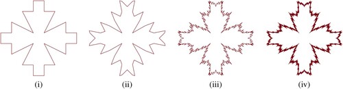
Figure 2 explains that the two types fractal curves generated by implementing the 8-point interpolating binary subdivision scheme after first, third, fifth, seventh, 9th, 11th and 13th subdivision level of the scheme along with initial polygon by using (7(7) $\begin{array}{rl}{f}_{2i}^{k+1}& =f_i^k,\\ f_{2i+1}^{k+1}& =-\eta f_{i-3}^k+(\mu +5\eta )f_{i-2}^k-(3\mu +9\eta +\frac{1}{16})f_{i-1}^k+(2\mu +5\eta +\frac{9}{16})f_i^k\\ & +(2\mu +5\eta +\frac{9}{16})f_{i+1}^k-(3\mu +9\eta +\frac{1}{16})f_{i+2}^k+(\mu +5\eta )f_{i+3}^k-\eta f_{i+4}^k.\end{array}$(7) ) at $\eta =-0.0576,\mu =3/256$ and $\eta =0.0576$ respectively. It is observed that the nature of fractal curves are totally different on the positive and negative range of parameters.

Figure 2. Fractals:(i) shows the initial polygon and (ii-xvi) shows the fractal curves at first, third, fifth, seventh, 9th, 11th and 13th subdivision level of the scheme (7(7) $\begin{array}{rl}{f}_{2i}^{k+1}& =f_i^k,\\ f_{2i+1}^{k+1}& =-\eta f_{i-3}^k+(\mu +5\eta )f_{i-2}^k-(3\mu +9\eta +\frac{1}{16})f_{i-1}^k+(2\mu +5\eta +\frac{9}{16})f_i^k\\ & +(2\mu +5\eta +\frac{9}{16})f_{i+1}^k-(3\mu +9\eta +\frac{1}{16})f_{i+2}^k+(\mu +5\eta )f_{i+3}^k-\eta f_{i+4}^k.\end{array}$(7) ) at $\eta =-0.0576,\mu =0.0576$ respectively.

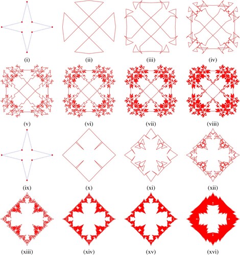
Figure 3 shows three fractal curves generated by using 8-point interpolating scheme after first and tenth level respectively. Figure 4(i) depicts their initial polygon, Figure 4(ii) shows the result obtained with $\eta =0.029$ and $\mu =0.029$ after first iteration and Figure 4(iii) shows the result obtained with $\eta =0.0345$ and $\mu =0.0345$ after tenth iteration.

Figure 3. (i) shows the initial polygon and Figure 4(ii-iii) shows the fractal curves at first and tenth subdivision level of the scheme (7(7) $\begin{array}{rl}{f}_{2i}^{k+1}& =f_i^k,\\ f_{2i+1}^{k+1}& =-\eta f_{i-3}^k+(\mu +5\eta )f_{i-2}^k-(3\mu +9\eta +\frac{1}{16})f_{i-1}^k+(2\mu +5\eta +\frac{9}{16})f_i^k\\ & +(2\mu +5\eta +\frac{9}{16})f_{i+1}^k-(3\mu +9\eta +\frac{1}{16})f_{i+2}^k+(\mu +5\eta )f_{i+3}^k-\eta f_{i+4}^k.\end{array}$(7) ) at $\eta =0.029,\mu =0.029$ respectively.

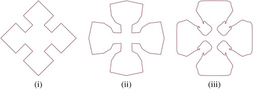
Figure 4. Fractals:(i) shows the initial polygon and (ii-iv) shows the fractal curves at first, forth and tenth subdivision level of the scheme (7(7) $\begin{array}{rl}{f}_{2i}^{k+1}& =f_i^k,\\ f_{2i+1}^{k+1}& =-\eta f_{i-3}^k+(\mu +5\eta )f_{i-2}^k-(3\mu +9\eta +\frac{1}{16})f_{i-1}^k+(2\mu +5\eta +\frac{9}{16})f_i^k\\ & +(2\mu +5\eta +\frac{9}{16})f_{i+1}^k-(3\mu +9\eta +\frac{1}{16})f_{i+2}^k+(\mu +5\eta )f_{i+3}^k-\eta f_{i+4}^k.\end{array}$(7) ) at $\eta =-0.029,\mu =-0.029$ respectively.

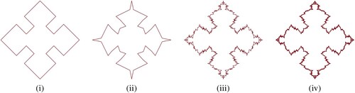
Figure 4(i) shows the initial polygon for a bearing and Figure 5(ii-iv) shows the actual bearing generated by setting the values of $\eta =-0.029,\mu =-0.029$ after first, fifth and tenth level respectively. The fractal curves in Figure 5(ii-iii) are just like the fractal antenna of Weissman [32] binary 6-point interpolating subdivision scheme that is generated with one parameter at $\mu =-0.099$.

Figure 5. Terrain like fractal curves by applying the 8-point binary interpolating subdivision scheme. (i) shows the initial polygon and (ii-iii) shows the fractal curves at fifth and ninth subdivision level of the scheme (7(7) $\begin{array}{rl}{f}_{2i}^{k+1}& =f_i^k,\\ f_{2i+1}^{k+1}& =-\eta f_{i-3}^k+(\mu +5\eta )f_{i-2}^k-(3\mu +9\eta +\frac{1}{16})f_{i-1}^k+(2\mu +5\eta +\frac{9}{16})f_i^k\\ & +(2\mu +5\eta +\frac{9}{16})f_{i+1}^k-(3\mu +9\eta +\frac{1}{16})f_{i+2}^k+(\mu +5\eta )f_{i+3}^k-\eta f_{i+4}^k.\end{array}$(7) ) at $\eta =-0.03,\mu =-0.03$ respectively.

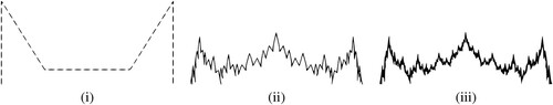
Figure 5 shows the terrain like fractal curves produced by applying the proposed 8-point interpolating binary scheme after fifth and ninth iteration. Figure 6(i) depicts the initial control polygon. Figure 6(ii-iii) which shows the results obtained by letting the values of $\eta =-0.03,\mu =-0.03$ respectively. From the above examples we can show that given the control polygon we can generate fractal curves by choosing the appropriate values of parameters according to theorem (5.1).

7. Conclusion

In this paper, A new 8-point binary interpolating subdivision scheme is constructed by using two parameters η and μ. Laurent polynomial is used to analysed the continuity of scheme. Fractal properties of this scheme with two parameters are discussed and relationship between the parameters and the limit fractal curve of 8-point binary interpolating subdivision scheme is also presented. The advantages of incorporating two shape parameters in a binary 8-point interpolatory subdivision scheme are rooted in the enhanced control, adaptability, and creative possibilities they offer for generating diverse and aesthetically pleasing fractal curves.

Disclosure statement

No potential conflict of interest was reported by the author(s).

References

- Rham Gde. Unpeu de mathématiques à propos d'unecourbe plane. Elemente Der Math. 1947;2:73–76.
- Ko KP, Lee BG, Yoon GJ. A study on the mask of interpolatory symmetric subdivision schemes. Appl Math Comput. 2007;187(2):609–621. doi: 10.1016/j.amc.2006.08.089
- Rehan K, Sabri MA. A combined ternary 4-point subdivision scheme. Appl Math Comput. 2016;276:278–283. doi: 10.1016/j.amc.2015.12.016
- Ghaffar A, Ullah Z, Bari M, et al. A new class of 2 m-point binary non-stationary subdivision schemes. Adv Differ Equ. 2019;2019(1):1–19. doi: 10.1186/s13662-019-2264-4
- Ghaffar A, Ullah Z, Bari M, et al. Family of odd point non-stationary subdivision schemes and their applications. Adv Differ Equ. 2019;2019(1):1–20. doi: 10.1186/s13662-019-2105-5
- Mustafa G, Khan F, Ghaffar A. The m-point approximating subdivision scheme. Lobachevskii J Math. 2009;30(2):138–145. doi: 10.1134/S1995080209020061
- Mustafa G, Ghaffar A, Khan F. The odd-point ternary approximating schemes. Am J Comput Math. 2011;01(02):111.118 doi: 10.4236/ajcm.2011.12011
- Mustafa G, Ghaffar A, Aslam M. A subdivision-regularization framework for preventing over fitting of data by a model. Appl Appl Math Int J. 2013;8(1):178–190.
- Ghaffar A, Mustafa G, Qin K. Unification and application of 3-point approximating subdivision schemes of varying arity. Open J Appl Sci. 2012;02(04):48–52. doi: 10.4236/ojapps.2012.24B012
- Ghaffar A, Mustafa G, Qin K. The 4-point a-ary approximating subdivision scheme. Open J Appl Sci. 2013;03(01):106–111. doi: 10.4236/ojapps.2013.31B1022
- Ghaffar A, Bari M, Ullah Z, et al. A new class of 2 q-point nonstationary subdivision schemes and their applications. Mathematics. 2019;7(7):639. doi: 10.3390/math7070639
- Ghaffar A, Iqbal M, Bari M, et al. Construction and application of nine-tic B-spline tensor product SS. Mathematics. 2019;7(8):675. doi: 10.3390/math7080675
- Ashraf P, Nawaz B, Baleanu D, et al. Analysis of geometric properties of ternary four-point rational interpolating subdivision scheme. Mathematics. 2020;8(3):338. doi: 10.3390/math8030338
- Ashraf P, Ghaffar A, Baleanu D, et al. Shape-Preserving properties of a relaxed four-Point interpolating subdivision scheme. Mathematics. 2020;8(5):806. doi: 10.3390/math8050806
- Ashraf P, Sabir M, Ghaffar A, et al. Shape-preservation of the four-point ternary interpolating non-stationary subdivision scheme. Front Phys. 2020;7:241. doi: 10.3389/fphy.2019.00241
- Shahzad A, Khan F, Ghaffar A, et al. A novel numerical algorithm to estimate the subdivision depth of binary subdivision schemes. Symmetry. 2020;12(1):66. doi: 10.3390/sym12010066
- Hussain SM, Rehman AU, Baleanu D, et al. Generalized 5-point approximating subdivision scheme of varying arity. Mathematics. 2020;8(4):474. doi: 10.3390/math8040474
- Ashraf P, Mustafa G, Ghaffar A, et al. Unified framework of approximating and interpolatory subdivision schemes for construction of class of binary subdivision schemes. J Funct Spaces. 2020;2020. 1 19. doi: 10.1155/2020/6677778
- Ashraf P, Mustafa G, Khan HA, et al. A shape-preserving variant of Lane-Riesenfeld algorithm. AIMS Math. 2021;6(3):2152–2170. doi: 10.3934/math.2021131
- Mustafa G, Ejaz ST, Baleanu D, et al. A subdivision-based approach for singularly perturbed boundary value problem. Adv Differ Equ. 2020;2020(1):1–20. doi: 10.1186/s13662-020-02732-8
- Bari M, Mustafa G, Ghaffar A, et al. Construction and analysis of unified 4-point interpolating nonstationary subdivision surfaces. Adv Differ Equ. 2021;2021(1):1–17. doi: 10.1186/s13662-021-03234-x
- Doo D, Sabin M. Behaviour of recursive division surfaces near extraordinary points. Comput-Aided Des. 1978;10(6):356–360. doi: 10.1016/0010-4485(78)90111-2
- Carpenter LC. Computer rendering of fractal curves and surfaces. ACM SIGGRAPH Comput Graphics. 1980;14(SI):9–9. doi: 10.1145/988447.988449
- Mandelbrot BB, Mandelbrot BB. The fractal geometry of nature. (Vol. New York: WH freeman; 1982. doi: 10.1002/esp.3290080415
- Bouboulis P, Dalla L. Fractal interpolation surfaces derived from fractal interpolation functions. J Math Anal Appl. 2007;336(2):919–936. doi: 10.1016/j.jmaa.2007.01.112
- Zheng H, Ye Z, Lei Y, et al. Fractal properties of interpolatory subdivision schemes and their application in fractal generation. Chaos Solit Fractals. 2007;32(1):113–123. doi: 10.1016/j.chaos.2005.10.075
- Zheng H, Ye Z, Chen Z, et al. Fractal range of a 3-point ternary interpolatory subdivision scheme with two parameters. Chaos Solit Fractals. 2007;32(5):1838–1845. doi: 10.1016/j.chaos.2005.12.017
- Mustafa G, Bari M, Jamil S. Engineering images designed by fractal subdivision scheme. SpringerPlus. 2016;5(1):1–11. doi: 10.1186/s40064-015-1659-2
- Peng K, Tan J, Li Z, et al. Fractal behavior of a ternary 4point rational interpolation subdivision scheme. Math Comput Appl. 2018;23(4):65. doi: 10.3390/mca23040065
- Bari M, Mustafa G, Hussain A. Fractal generation by 7-Point binary approximating subdivision scheme. Int J Appl Phys Math. 2018;8(4):105–111. doi: 10.17706/ijapm.2018.8.4.105-111
- Yao SW, Ashraf P, Ghaffar A, et al. Fractal and convexity analysis of the quaternary 4-point scheme and its applications. Fractals. 2023;31(10):1–14. doi: 10.1142/S0218348X23400881
- Weissman A. A 6-point interpolatory subdivision scheme for curve design. University of Tel-Aviv. 1989.
- Deslauriers G, Dubuc S. Symmetric iterative interpolation processes. In Constructive approximation (pp. 49–68). Springer, Boston, MA. 1989.