The complex dynamical behaviour of fractal-fractional forestry biomass system

Abstract

In this research, we aim to propose a non-integer order mathematical model that illustrates the detrimental impact of illegal logging on forest biomass. The model is based on the idea that soil nutrients play a vital role in the growth of forestry biomass. However, the growth of forestry biomass is hindered by the harvesting of trees for industrial expansion. To develop the model, we use a fractional order approach, which allows us to explore the impact of conservation efforts on the extension of industries. If the amount of forestry biomass that is illegally harvested exceeds a certain threshold, the system becomes unstable. To investigate the proposed model's solution, we use fixed-point theory, which is highly effective in determining the existence and uniqueness of the solution. We also use Ulam-Hyers stability to analyse the stability of the proposed model. We have also employed new versions of fractional numerical techniques using power law and exponential decay. Our proposed model provides more details through numerical calculations with fractional orders different from integer ones. Moreover, we have addressed all significant solution behaviours in the fractal-fractional system and parameter values. The graphical representation offers a better understanding of the forestry biomass model, allowing us to identify the direction and stability of solutions. From various perspectives, we analysed the features of solutions to this fractal-fractional model for stopping illegal logging.

Keywords:

• Forestry biomass model
• fractal-fractional Caputo derivative
• fractal-fractional Caputo-Fabrizio derivative
• existence and uniqueness
• Ulam-Hyers stability
• numerical method

2020 Mathematics Subject Classifications:

• 37-03
• 37D4

1. Introduction

An area of mathematics known as fractional calculus focuses on implementations for arbitrary order integrals and derivatives. Conversely, there was limited conversation surrounding fractional calculus, especially regarding its practical uses. Nonetheless, fractional calculus has emerged as one of the most sought-after academic fields in recent years, thanks to its theoretical progress and potential applications in engineering and scientific disciplines [1]. A system's fundamental dynamics depend on the past behaviour of real-world mathematical modelling problems [2]. As a result, the system's future depends on its current state and history of state and dependents. The integer order differential operator cannot capture the behaviour of such systems in hereditary terms. In contrast, the fractional order derivative, which is nonlocal, is a valuable tool for modelling nonlocal occurrences in both space and time. Non-integer order operators describe every step of the process study in the proposed model. Because of this, such operators are good tools for describing the systems' memory and hereditary characteristics. The nonlocal property of non-integer order operators contributed to the success of fractional calculus. Mathematically modelling real-world systems in terms of fractional-order derivatives generates several fractional-order differential equations frequently intractable by analytical means, leading to high computational expenses to render such solutions realistic [3]. The Mittag-Leffler function plays a distinctive and challenging role in fractional calculus.

Researchers have devised numerical and approximative analytical methodologies for solving differential equations since analytical solutions are either unavailable or limited to complex mathematical functions [4]. The range of numerical methods for differential equations is limited because of many of the challenges in their analysis, but the researcher has developed new numerical techniques. Classical initial conditions are used in fractional differential equations involving the Caputo fractional derivative, which are understandable and can be accurately measured. Researchers present several fractional derivatives, the most popular and often used non-classical derivatives of Caputo, Atangana-Baleanu, and Caputo-Fabrizio (C-F) [5, 6]. There has been a recent development in kernels of fractional fractal derivatives in different forms, such as power law, exponential decay, and the Mittag-Leffler function [7]. One advantage of these differential operators is that they depend on two orders: the fractional order and the fractal dimension. The fractal-fractional (F-F) operator, in the sense of Caputo and C-F, effectively conveys complexities that are difficult to depict using traditional fractional operators. The F-F approach has been used to solve numerous mathematical models. Many analysis fields, including banking [8] and disease models [9, 10], frequently employ the F-F operator [11].

The Predictor-Corrector technique determines the numerical solution of fractional differential equations with several examples of this new fractional derivative [12, 13]. This altered form of the Predictor-Corrector method non-uniform grid is an emphatic weapon for investigating fractional differential equations. Two dis-contiguous perspectives serve as the foundation for the methodologies employed in the numerical simulation of chaotic fractional order systems. ‘Time domain methods’ are techniques used to directly approximate the response of a fractional order system when solving differential equations numerically. The enhanced Adams-Bashforth Moulton algorithm, presented based on the predictor-corrector scheme, is one of the finest algorithms in this area [14, 15]. The approach can effectively address the stability of non-linear systems of equations that easy-to-handle chaotic problems, which is highly significant. Various numerical methods that utilize fractional order operators to define these real-life issues differ and are customized.

There have been several numerical techniques developed to handle problems that involve fractional initial values. Mathematical modelling is a method used to depict reality or define present circumstances. It is also used to make predictions based on scientific principles about future possibilities. However, mathematical modelling has some constraints. It's challenging to estimate with many parameters and functions within constraints. The accuracy of mathematical modelling depends on how well it describes a particular issue [16]. For instance, several variables can be ignored when simulating infectious diseases, such as weather and the health of each person in the community. Identifying the variables that impact modelling is essential to minimize errors and predict how the disease evolves.

Since the dawn of time, people have faced illnesses and combated them in their local communities. Science and technology have brought about rapid changes that make life more convenient and comfortable. Unfortunately, human progress has also led to significant deterioration of the natural environment in virtually every part of the world. Human growth in science and technology has caused many natural phenomena, such as cultural norms, modern agriculture, education, transportation, and others, to undergo significant changes [17]. Advances in technology have made it possible to develop genetically changed food products. However, humans' overuse of natural resources is leading to the extinction of several plant and animal species. Attributing all the world's problems to pandemics when seasonal fluctuations significantly impact the dynamics of various species populations is unfair. How chronic wasting disease spreads among animals in a population and how environmental factors affect this illness [18]. A mathematical model of non-integer predator and prey that includes two predators coexisting on a single prey in this article [19].

Palm oil is the most commonly used vegetable oil worldwide and can be found in many packaged foods, stores, and cosmetics. It is an efficient and cost-effective oil that requires less land than other oils to produce the same amount of energy. However, the destruction of forests in some countries has led to widespread concern and government action because of the adverse effects on habitats and air quality. Illegal logging, which involves harvesting wood against the law, is a significant cause of deforestation, soil erosion, and biodiversity loss. This kind of logging can be carried out using dishonest means to acquire permission to use protected forests, cutting down protected species without a license, or exceeding the permitted amount of timber. These environmental problems can lead to even more severe catastrophes like climate change and ecological degradation. Forest degradation and deforestation are significant issues in developing countries, and the trade in illegally harvested wood products contributes to these problems. The soil's nutritional balance is crucial for maintaining productivity, as trees rely on nutrients from the soil for growth and maintenance. The paper's author proposes a mathematical framework for managing forest biomass, focussing on the example of Indonesia, which is affected by forest clearance because of mining and oil plantations [20].

Most illicit cutting down, timber-prohibited activity, and the utilization of fossil fuels for cooking are to blame for the misappropriation of forestry biomass in underdeveloped countries. Domestic demand is one of the reasons that consume a sizable amount of illegal timber. An effort is made to build a mathematical model, stating tax as the control measure for lawful logging, taking into account the severity of the issue experienced by the prevalence of developing countries. Mathematical models are widely used when studying fisheries and forestry population conservation. The nineteenth century saw the introduction of research on forestry and fishing populations that considered economic factors. Taxes are a mechanism by which regulatory and governmental bodies modify the costs associated with access to forest resources. To encourage operators to maintain the value of the resources in the forest industry, keeping the tax rate in line with profitability incentives is essential. This will motivate them to improve their performance, even if they cannot meet the new requirements. In ecology, the functional response is crucial for illustrating the relationship between a predator and its prey. It has been demonstrated in the paper [21] that the system undergoes Hopf-bifurcation when Holling type IV functional response and nonlinear age-selective prey harvesting utilizing the prey-generalist predator model are taken into account. Before now, many mathematical models for the utilization and preservation of forestry biomass were put out, taking into interpretation the impact of population, technology, and pollution. In this paper [22], a theoretical framework and mathematical model that combines the population of humans with both reserved and unreserved forest biomass is put forth in response to the rise in atmospheric carbon dioxide.

A deeper understanding of complex systems, such as biomass dynamics, can be achieved using fractional derivatives, extending the concept of differentiation to non-integer orders. However, traditional calculus-based derivatives are still helpful as a reference point for comparison. In this study, we compare the effectiveness of these methods and investigate the dynamics of forestry biomass, building upon previous research. By doing so, we can better understand the role of forestry biomass in environmental sustainability, and the analysis yields new insights. F-F derivative provides a mathematical basis for characterizing the complex, self-similar nature of various elements in a forest, such as branches, leaves, and roots, at different observational levels. With the help of the fractional operator and the Lagrangian interpolation approach, forestry models can accurately depict the intricate configurations of biomass elements, leading to more reliable and precise biomass estimation. Using numerical methods also enables the measurement of these patterns across scales, enhancing the spatial accuracy of biomass models and accounting for the spatial heterogeneity, the variation in biomass distribution across different environmental conditions and locations, a defining characteristic of forest ecosystems. This approach offers a scalable and continuous way of describing the geographical distribution of biomass, particularly in complex forest environments. These methods provide flexibility to researchers, allowing them to adapt their methodologies to fit different forest types, observational scales, and modelling goals. The biomass model can use these techniques in big datasets and intricate spatial structures.

An ordered breakdown of the complete work is given in the following sections: concepts related to fractional calculus are defined in Section 2. Section 3 discusses the fractal-fractional model of forestry biomass. We address the model solution's stability, existence, and uniqueness in Sections 4 and 4.1. Numerical methods are presented in Section 5 for a fractional-order forestry biomass model. Numerical simulation and discussion are found in Section 6. The conclusion is found in Section 7.

2. Preliminaries

This part thoroughly looks at several definitions and theorems about fractional operators. There are also some fractal-fractional calculus-related outcomes. ψ denotes the fractional-order and φ represents the fractal-dimension.

Definition 2.1

[23, 24]

We suppose that $(a,b)$ be an open interval, and $\mathcal{W}\left(t\right)$ be a continuous function and along with $\psi ,\phi \in (0,1],$ in the R-L derivative with power law kernel is (1) ${}^{\mathrm{FFP}}{}_0{\mathfrak{D}}_{0,t}^{\psi ,\phi }\left(\mathcal{W}\right(t\left)\right)=\frac{1}{\mathrm{\Gamma }(k-\psi )}\frac{\mathrm{d}}{\mathrm{d}{t}^{\phi }}{\int }_0^t(t-z{)}^{k-\psi -1}\mathcal{W}(z)\mathrm{d}z,$(1) with $k-1<\psi ,\phi \le k\in \mathbb{M}$ and $\frac{\mathrm{d}\mathcal{W}\left(z\right)}{\mathrm{d}{z}^{\phi }}=\underset{t\to z}{lim}\frac{\mathcal{W}\left(t\right)-\mathcal{W}\left(z\right)}{t^{\phi }-z^{\phi }}.$

Definition 2.2

[23, 24]

We suppose that $(a,b)$ be an open interval, and $\mathcal{W}\left(t\right)$ be a continuous function and along with $\psi ,\phi \in (0,1],$ in the R-L derivative with exponentially decaying kernel is (2) ${}^{\mathrm{FFE}}{}_0{\mathfrak{D}}_{0,t}^{\psi ,\phi }\left(\mathcal{W}\right(t\left)\right)=\frac{B\left(\psi \right)}{1-\psi }\frac{\mathrm{d}}{\mathrm{d}{t}^{\phi }}{\int }_0^t\exp \left(\frac{-\psi }{1-\psi }\right(t-z\left)\right)\mathcal{W}\left(z\right)\mathrm{d}z,$(2) and $B\left(0\right)=B\left(1\right)=1.$

Definition 2.3

[23, 24]

We suppose that $(a,b)$ be an open interval, and $\mathcal{W}\left(t\right)$ be a continuous function and along with $\psi ,\phi \in (0,1],$ integral with power law kernel is (3) ${}^{\mathrm{FFP}}{}_0{\mathfrak{I}}_{0,t}^{\psi ,\phi }\left(\mathcal{W}\right(t\left)\right)=\frac{\phi }{\mathrm{\Gamma }\left(\psi \right)}{\int }_0^t(t-z{)}^{\psi -1}{z}^{\phi -1}\mathcal{W}(z)\mathrm{d}z.$(3)

Definition 2.4

[23, 24]

We suppose that $(a,b)$ be an open interval, and $\mathcal{W}\left(t\right)$ be a continuous function and along with $\psi ,\phi \in (0,1],$ integral with exponential decay kernel is (4) ${}^{\mathrm{FFE}}{}_0{\mathfrak{I}}_{0,t}^{\psi ,\phi }\left(\mathcal{W}\right(t\left)\right)=\frac{\phi (1-\psi )t^{\phi -1}\mathcal{W}\left(t\right)}{B\left(\psi \right)}+\frac{\mathrm{\psi \phi }}{B\left(\psi \right)}{\int }_0^t{z}^{\phi -1}\mathcal{W}\left(z\right)\mathrm{d}z.$(4)

Theorem 2.1

[25, 26]

Suppose that $\mathrm{\Theta }:\mathrm{{\rm Y}}\to \mathrm{{\rm Y}}$ be an operator and completely continuous. Let $B\left(\mathrm{\Theta }\right)=\{N\in \mathrm{{\rm Y}}:N=\zeta \mathrm{\Theta }(N),\zeta \in [0,1\left]\right\}.$The operator Θ has at least one fixed point or the set $B\left(\mathrm{\Theta }\right)$ is unbounded.

3. The mathematical formulation of the forestry biomass system

Mathematical biology is a field that combines mathematical methods and biological research to create models. Although it's crucial to use mathematics in biology because of the increasingly quantitative nature of the field, the number of research groups and individuals working in this area is limited. Modern applications of mathematics in mathematical biology are fascinating and rapidly increasing. In the article [27], we see author have suggested and studied some models while taking into interpretation various elements that take advantage of the natural population. We've taken into account the issue of illegal logging as one of the factors contributing to the absorption and degradation of forest biomass. When the author developed the model also took into reflection the approach put forth in this paper [28]. They took into account alternative foods for predators. They found that in some circumstances is a shortage of prey, a rise in focal prey is seen if the predator uses fewer alternatives, and when the prey population approaches the carrying capacity, consumption of choices tends to zero. In developing the mathematical model, a similar idea of alternate resources in the development of forestry biomass is taken into account. In the proposed model, N denotes the nutrient density, and the forestry biomass is represented by P. E denotes the measure of effort intensity, and the industrial density is represented by the I. Regarding the nutrient-dependent growth rate, it is predicted that the biomass of the forest will increase logistically. The terms $q_1\mathrm{PE}$ and $d_2\mathrm{PE}$ represent legal and illicit tree-cutting and are directly affected by these trees cutting the loss of forestry biomass. Furthermore, it is considered that taxes levied by the government result in fewer industries, which help to preserve forest biomass. In addition, it is also believed that as taxes rise, the alternatives aid in the expansion of the industries denoted by the term ‘$\mathrm{\mu I}(1-\frac{p}{k})$’ in the equation for I. Additionally, it is presumed that when there are alternatives, industries expand the fastest. Because the forestry population will be gotten near its carrying limit, alternate consumption tends to be zero. The state transition flow diagram for the model formulation is provided in Figure 1 after carefully considering the assumptions. Q represents the constant input rate of nutrients, and β denotes the utilization rate of nutrients by forestry biomass. $r\left(N\right)$ denotes the modified intrinsic growth rate of forestry biomass, and $d_1$ represents the washout rate of nutrients. K symbolizes the carrying capacity of forestry biomass, and γ signifies the new plantation rate. c denotes the fixed cost per unit of effort expended to harvest forestry biomass, and $d_2$ represents the illegal logging of forestry biomass. $q_1$ symbolizes the harvesting rate of forestry biomass, and $d_3$ signifies the reduction rate of industries. α means the rate of growth industries on account of efforts, and μ represents the maximum growth due to alternative industries. p and τ symbolize the fixed price and tax per unit of forestry biomass respectively.

Figure 1. A diagrammatic graph presentation of the forestry biomass relations of given the system is like as. In the flow diagram, $f\left(P\right)$ represents the function of forestry biomass (trees), which combines logistic growth and new plantation, described as $f\left(P\right)=\mathrm{rP}(1-\frac{P}{K})+\mathrm{\gamma P}$, $f_1(N,P)=r_{0}N(1-\frac{P}{K})$, $f_2(P,E)$ is the function of forestry biomass and industrial density through legal and illegal logging, $f_2(P,E)=d_1\mathrm{PE}+q_1\mathrm{PE}$ and $f_3(P,I)=\frac{\mathrm{\mu IP}}{K}.$ With the help of arrows and labels, the intensity and relationship between the compartments are marked.

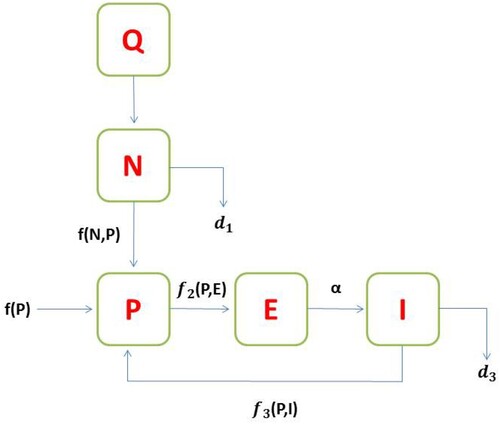
The four differential equations listed below describe the model [29]. (5) $\begin{array}{rl}\frac{\mathrm{d}N}{\mathrm{d}t}& =Q-\text{β}P-d_{1}N,\\ \frac{\mathrm{d}P}{\mathrm{d}t}& =r\left(N\right)P(1-\frac{P}{K})-q_1\mathrm{PE}-d_2\mathrm{PE}+\mathrm{\gamma P},v\\ \frac{\mathrm{d}E}{\mathrm{d}t}& =q_1(p-\tau )\mathrm{PE}+p{d}_2\mathrm{PE}-\mathrm{cE},\\ \frac{\mathrm{d}I}{\mathrm{d}t}& =\mathrm{\alpha E}+\mathrm{\mu I}(1-\frac{P}{K})-d_{3}I,\end{array}$(5) the proposed model has the following initial conditions: $N\left(0\right)=N_0,P\left(0\right)=P_0,E\left(0\right)=E_0,I\left(0\right)=I_0,$where $r\left(N\right)=r+r_{0}N$.

We apply the Fractal-Fractional (F-F) Caputo-Fabrizio (C-F) derivative [10] in the model (5(5) $\begin{array}{rl}\frac{\mathrm{d}N}{\mathrm{d}t}& =Q-\text{β}P-d_{1}N,\\ \frac{\mathrm{d}P}{\mathrm{d}t}& =r\left(N\right)P(1-\frac{P}{K})-q_1\mathrm{PE}-d_2\mathrm{PE}+\mathrm{\gamma P},v\\ \frac{\mathrm{d}E}{\mathrm{d}t}& =q_1(p-\tau )\mathrm{PE}+p{d}_2\mathrm{PE}-\mathrm{cE},\\ \frac{\mathrm{d}I}{\mathrm{d}t}& =\mathrm{\alpha E}+\mathrm{\mu I}(1-\frac{P}{K})-d_{3}I,\end{array}$(5) ), we obtain (6) $\begin{array}{rl}{}^{\mathrm{FFE}}{}_{0+}{\mathfrak{D}}_t^{\psi ,\phi }N\left(t\right)& =Q-\text{β}P-d_{1}N,\\ {}^{\mathrm{FFE}}{}_{0+}{\mathfrak{D}}_t^{\psi ,\phi }P\left(t\right)& =r\left(N\right)P(1-\frac{P}{K})-q_1\mathrm{PE}-d_2\mathrm{PE}+\mathrm{\gamma P},\\ {}^{\mathrm{FFE}}{}_{0+}{\mathfrak{D}}_t^{\psi ,\phi }E\left(t\right)& =q_1(p-\tau )\mathrm{PE}+p{d}_2\mathrm{PE}-\mathrm{cE},\\ {}^{\mathrm{FFE}}{}_{0+}{\mathfrak{D}}_t^{\psi ,\phi }I\left(t\right)& =\mathrm{\alpha E}+\mathrm{\mu I}(1-\frac{P}{K})-d_{3}I,\end{array}$(6) the proposed model has the following initial conditions: $N\left(0\right)=N_0,P\left(0\right)=P_0,E\left(0\right)=E_0,I\left(0\right)=I_0.$

4. Existence and uniqueness of the solution

The existence and uniqueness theory [30] for the forestry biomass model is constructed in this section. The system (6(6) $\begin{array}{rl}{}^{\mathrm{FFE}}{}_{0+}{\mathfrak{D}}_t^{\psi ,\phi }N\left(t\right)& =Q-\text{β}P-d_{1}N,\\ {}^{\mathrm{FFE}}{}_{0+}{\mathfrak{D}}_t^{\psi ,\phi }P\left(t\right)& =r\left(N\right)P(1-\frac{P}{K})-q_1\mathrm{PE}-d_2\mathrm{PE}+\mathrm{\gamma P},\\ {}^{\mathrm{FFE}}{}_{0+}{\mathfrak{D}}_t^{\psi ,\phi }E\left(t\right)& =q_1(p-\tau )\mathrm{PE}+p{d}_2\mathrm{PE}-\mathrm{cE},\\ {}^{\mathrm{FFE}}{}_{0+}{\mathfrak{D}}_t^{\psi ,\phi }I\left(t\right)& =\mathrm{\alpha E}+\mathrm{\mu I}(1-\frac{P}{K})-d_{3}I,\end{array}$(6) ) is now rewrite, looking like this: (7) $\begin{array}{rl}& {}^{\mathrm{CF}}{}_{0+}{\mathfrak{D}}_t^{\psi }N\left(t\right)=\phi t^{\phi -1}\left[{\mathbb{D}}_1\right(t,N\left(t\right),P\left(t\right),E\left(t\right),I\left(t\right)\left)\right],\\ & {}^{\mathrm{CF}}{}_{0+}{\mathfrak{D}}_t^{\psi }P\left(t\right)=\phi t^{\phi -1}\left[{\mathbb{D}}_2\right(t,N\left(t\right),P\left(t\right),E\left(t\right),I\left(t\right)\left)\right],\\ & {}^{\mathrm{CF}}{}_{0+}{\mathfrak{D}}_t^{\psi }E\left(t\right)=\phi t^{\phi -1}\left[{\mathbb{D}}_3\right(t,N\left(t\right),P\left(t\right),E\left(t\right),I\left(t\right)\left)\right],\\ & {}^{\mathrm{CF}}{}_{0+}{\mathfrak{D}}_t^{\psi }I\left(t\right)=\phi t^{\phi -1}\left[{\mathbb{D}}_4\right(t,N\left(t\right),P\left(t\right),E\left(t\right),I\left(t\right)\left)\right],\end{array}$(7) where $\{\begin{array}{l}{\mathbb{D}}_1(t,N(t),P(t),E(t),I(t\left)\right)=Q-\text{β}P-d_{1}N,\\ {\mathbb{D}}_2(t,N(t),P(t),E(t),I(t\left)\right)=r\left(N\right)P(1-\frac{P}{K})-q_1\mathrm{PE}-d_2\mathrm{PE}+\mathrm{\gamma P},\\ {\mathbb{D}}_3(t,N(t),P(t),E(t),I(t\left)\right)=q_1(p-\tau )\mathrm{PE}+p{d}_2\mathrm{PE}-\mathrm{cE},\\ {\mathbb{D}}_4(t,N(t),P(t),E(t),I(t\left)\right)=\mathrm{\alpha E}+\mathrm{\mu I}(1-\frac{P}{K})-d_{3}I.\end{array}$The system (7(7) $\begin{array}{rl}& {}^{\mathrm{CF}}{}_{0+}{\mathfrak{D}}_t^{\psi }N\left(t\right)=\phi t^{\phi -1}\left[{\mathbb{D}}_1\right(t,N\left(t\right),P\left(t\right),E\left(t\right),I\left(t\right)\left)\right],\\ & {}^{\mathrm{CF}}{}_{0+}{\mathfrak{D}}_t^{\psi }P\left(t\right)=\phi t^{\phi -1}\left[{\mathbb{D}}_2\right(t,N\left(t\right),P\left(t\right),E\left(t\right),I\left(t\right)\left)\right],\\ & {}^{\mathrm{CF}}{}_{0+}{\mathfrak{D}}_t^{\psi }E\left(t\right)=\phi t^{\phi -1}\left[{\mathbb{D}}_3\right(t,N\left(t\right),P\left(t\right),E\left(t\right),I\left(t\right)\left)\right],\\ & {}^{\mathrm{CF}}{}_{0+}{\mathfrak{D}}_t^{\psi }I\left(t\right)=\phi t^{\phi -1}\left[{\mathbb{D}}_4\right(t,N\left(t\right),P\left(t\right),E\left(t\right),I\left(t\right)\left)\right],\end{array}$(7) ) rewrite as (8) $\begin{array}{rl}{}^{\mathrm{CF}}{}_0{\mathfrak{D}}_{0,t}^{\psi }\mathcal{Q}\left(t\right)& =\phi t^{\phi -1}\mathbb{D}(t,\mathcal{Q}(t\left)\right)\\ \mathcal{Q}\left(0\right)& ={\mathcal{Q}}_0.\end{array}$(8) We employ the F-F integral in the C-F sense, we obtain (9) $\mathcal{Q}\left(t\right)=\mathcal{Q}\left(0\right)+\frac{\phi (1-\psi )}{B\left(\psi \right)}{t}^{\phi -1}\mathbb{D}(t,\mathcal{Q}(t\left)\right)+\frac{\mathrm{\psi \phi }}{B\left(\psi \right)}{\int }_0^t{u}^{\phi -1}\mathbb{D}(u,\mathcal{Q}(u\left)\right)\mathrm{d}u,$(9) where $\mathcal{Q}\left(t\right)=\{\begin{array}{l}N\left(t\right)\\ P\left(t\right)\\ E\left(t\right)\\ I\left(t\right)\end{array}\mathbb{D}(t,\mathcal{Q}(t\left)\right)=\{\begin{array}{l}{\mathbb{D}}_1(t,N(t),P(t),E(t),I(t\left)\right)\\ {\mathbb{D}}_2(t,N(t),P(t),E(t),I(t\left)\right)\\ {\mathbb{D}}_3(t,N(t),P(t),E(t),I(t\left)\right)\\ {\mathbb{D}}_4(t,N(t),P(t),E(t),I(t\left)\right)\end{array}$In the system (7(7) $\begin{array}{rl}& {}^{\mathrm{CF}}{}_{0+}{\mathfrak{D}}_t^{\psi }N\left(t\right)=\phi t^{\phi -1}\left[{\mathbb{D}}_1\right(t,N\left(t\right),P\left(t\right),E\left(t\right),I\left(t\right)\left)\right],\\ & {}^{\mathrm{CF}}{}_{0+}{\mathfrak{D}}_t^{\psi }P\left(t\right)=\phi t^{\phi -1}\left[{\mathbb{D}}_2\right(t,N\left(t\right),P\left(t\right),E\left(t\right),I\left(t\right)\left)\right],\\ & {}^{\mathrm{CF}}{}_{0+}{\mathfrak{D}}_t^{\psi }E\left(t\right)=\phi t^{\phi -1}\left[{\mathbb{D}}_3\right(t,N\left(t\right),P\left(t\right),E\left(t\right),I\left(t\right)\left)\right],\\ & {}^{\mathrm{CF}}{}_{0+}{\mathfrak{D}}_t^{\psi }I\left(t\right)=\phi t^{\phi -1}\left[{\mathbb{D}}_4\right(t,N\left(t\right),P\left(t\right),E\left(t\right),I\left(t\right)\left)\right],\end{array}$(7) ), we employ the F-F integral in the C-F sense, we obtain (10) $\begin{array}{rl}N\left(t\right)& =N\left(0\right)+\frac{\phi (1-\psi )}{B\left(\psi \right)}{t}^{\phi -1}{\mathbb{D}}_1(t,N(t),P(t),E(t),I(t\left)\right)\\ & +\frac{\mathrm{\psi \phi }}{B\left(\psi \right)}{\int }_0^t{u}^{\phi -1}{\mathbb{D}}_1(u,N(u),P(u),E(u),I(u\left)\right)\mathrm{d}u,\\ P\left(t\right)& =P\left(0\right)+\frac{\phi (1-\psi )}{B\left(\psi \right)}{t}^{\phi -1}{\mathbb{D}}_2(t,N(t),P(t),E(t),I(t\left)\right)\\ & +\frac{\mathrm{\psi \phi }}{B\left(\psi \right)}{\int }_0^t{u}^{\phi -1}{\mathbb{D}}_2(u,N(u),P(u),E(u),I(u\left)\right)\mathrm{d}u,\\ E\left(t\right)& =E\left(0\right)+\frac{\phi (1-\psi )}{B\left(\psi \right)}{t}^{\phi -1}{\mathbb{D}}_3(t,N(t),P(t),E(t),I(t\left)\right)\\ & +\frac{\mathrm{\psi \phi }}{B\left(\psi \right)}{\int }_0^t{u}^{\phi -1}{\mathbb{D}}_3(u,N(u),P(u),E(u),I(u\left)\right)\mathrm{d}u,\\ I\left(t\right)& =I\left(0\right)+\frac{\phi (1-\psi )}{B\left(\psi \right)}{t}^{\phi -1}{\mathbb{D}}_4(t,N(t),P(t),E(t),I(t\left)\right)\\ & +\frac{\mathrm{\psi \phi }}{B\left(\psi \right)}{\int }_0^t{u}^{\phi -1}{\mathbb{D}}_4(u,N(u),P(u),E(u),I(u\left)\right)\mathrm{d}u.\end{array}$(10) We use the fixed point theory to prove the uniqueness and existence of the solution. A Banach space can be defined as follows ${\mathrm{{\rm Y}}}_n$ = $\mathbb{J}[0,\mathbb{T}]$ is space of all functions N, P, E, I respectively to $n=1,2,\dots ,4.$ ${\mathrm{{\rm Y}}}_n$ a Banach space with the norm $\Vert N\Vert =\underset{t\in [0,\mathbb{T}]}{max}|N\left(t\right)|,$ $\Vert P\Vert =\underset{t\in [0,\mathbb{T}]}{max}|P\left(t\right)|,$ $\Vert E\Vert =\underset{t\in [0,\mathbb{T}]}{max}|E\left(t\right)|$ $\Vert I\Vert =\underset{t\in [0,\mathbb{T}]}{max}|I\left(t\right)|$ respectively to $n=1,2,3,4.$ Consequently, the norm in the product space is created as $\Vert (N,P,E,I)\Vert =\Vert N\Vert +\Vert P\Vert +\Vert E\Vert +\Vert I\Vert .$Banach space is defined as $\mathrm{{\rm Y}}=({\mathrm{{\rm Y}}}_1\times {\mathrm{{\rm Y}}}_2\times {\mathrm{{\rm Y}}}_3\times {\mathrm{{\rm Y}}}_4,\Vert (N,P,E,I)\Vert ).$We suppose the operator $\mathrm{\Theta }:\mathrm{{\rm Y}}\to \mathrm{{\rm Y}}$ is defined in system (10(10) $\begin{array}{rl}N\left(t\right)& =N\left(0\right)+\frac{\phi (1-\psi )}{B\left(\psi \right)}{t}^{\phi -1}{\mathbb{D}}_1(t,N(t),P(t),E(t),I(t\left)\right)\\ & +\frac{\mathrm{\psi \phi }}{B\left(\psi \right)}{\int }_0^t{u}^{\phi -1}{\mathbb{D}}_1(u,N(u),P(u),E(u),I(u\left)\right)\mathrm{d}u,\\ P\left(t\right)& =P\left(0\right)+\frac{\phi (1-\psi )}{B\left(\psi \right)}{t}^{\phi -1}{\mathbb{D}}_2(t,N(t),P(t),E(t),I(t\left)\right)\\ & +\frac{\mathrm{\psi \phi }}{B\left(\psi \right)}{\int }_0^t{u}^{\phi -1}{\mathbb{D}}_2(u,N(u),P(u),E(u),I(u\left)\right)\mathrm{d}u,\\ E\left(t\right)& =E\left(0\right)+\frac{\phi (1-\psi )}{B\left(\psi \right)}{t}^{\phi -1}{\mathbb{D}}_3(t,N(t),P(t),E(t),I(t\left)\right)\\ & +\frac{\mathrm{\psi \phi }}{B\left(\psi \right)}{\int }_0^t{u}^{\phi -1}{\mathbb{D}}_3(u,N(u),P(u),E(u),I(u\left)\right)\mathrm{d}u,\\ I\left(t\right)& =I\left(0\right)+\frac{\phi (1-\psi )}{B\left(\psi \right)}{t}^{\phi -1}{\mathbb{D}}_4(t,N(t),P(t),E(t),I(t\left)\right)\\ & +\frac{\mathrm{\psi \phi }}{B\left(\psi \right)}{\int }_0^t{u}^{\phi -1}{\mathbb{D}}_4(u,N(u),P(u),E(u),I(u\left)\right)\mathrm{d}u.\end{array}$(10) ), then we have (11) $\mathrm{\Theta }(N,P,E,I)=\left(\begin{array}{c}{\mathrm{\Theta }}_1(N,P,E,I)\left(t\right)\\ {\mathrm{\Theta }}_2(N,P,E,I)\left(t\right)\\ {\mathrm{\Theta }}_3(N,P,E,I)\left(t\right)\\ {\mathrm{\Theta }}_4(N,P,E,I)\left(t\right)\end{array}\right),$(11) where (12) $\begin{array}{rl}{\mathrm{\Theta }}_1(N,P,E,I)\left(t\right)& =N\left(0\right)+\frac{\phi (1-\psi )}{B\left(\psi \right)}{t}^{\phi -1}{\mathbb{D}}_1(t,N(t),P(t),E(t),I(t\left)\right)\\ & +\frac{\mathrm{\psi \phi }}{B\left(\psi \right)}{\int }_0^t{u}^{\phi -1}{\mathbb{D}}_1(u,N(u),P(u),E(u),I(u\left)\right)\mathrm{d}u,\\ {\mathrm{\Theta }}_2(N,P,E,I)\left(t\right)& =P\left(0\right)+\frac{\phi (1-\psi )}{B\left(\psi \right)}{t}^{\phi -1}{\mathbb{D}}_2(t,N(t),P(t),E(t),I(t\left)\right)\\ & +\frac{\mathrm{\psi \phi }}{B\left(\psi \right)}{\int }_0^t{u}^{\phi -1}{\mathbb{D}}_2(u,N(u),P(u),E(u),I(u\left)\right)\mathrm{d}u,\\ {\mathrm{\Theta }}_3(N,P,E,I)\left(t\right)& =E\left(0\right)+\frac{\phi (1-\psi )}{B\left(\psi \right)}{t}^{\phi -1}{\mathbb{D}}_3(t,N(t),P(t),E(t),I(t\left)\right)\\ & +\frac{\mathrm{\psi \phi }}{B\left(\psi \right)}{\int }_0^t{u}^{\phi -1}{\mathbb{D}}_3(u,N(u),P(u),E(u),I(u\left)\right)\mathrm{d}u,\\ {\mathrm{\Theta }}_4(N,P,E,I)\left(t\right)& =I\left(0\right)+\frac{\phi (1-\psi )}{B\left(\psi \right)}{t}^{\phi -1}{\mathbb{D}}_4(t,N(t),P(t),E(t),I(t\left)\right)\\ & +\frac{\mathrm{\psi \phi }}{B\left(\psi \right)}{\int }_0^t{u}^{\phi -1}{\mathbb{D}}_4(u,N(u),P(u),E(u),I(u\left)\right)\mathrm{d}u.\end{array}$(12)

Theorem 4.1

Let assume that the functions ${\mathbb{D}}_n:$ $\mathcal{I}\times {\mathcal{R}}^4\to \mathcal{R}$ are continuous and constants are ${\mathcal{V}}_{1,{\mathbb{D}}_n},$ ${\mathcal{V}}_{2,{\mathbb{D}}_n},$ ${\mathcal{V}}_{3,{\mathbb{D}}_n}$ and ${\mathcal{V}}_{4,{\mathbb{D}}_n}>0,$ such that ∀$N,\hat{N},P,\hat{P},E,\hat{E},I,\hat{I}\in \mathrm{{\rm Y}},$ where $\mathcal{I}=[0,\mathbb{T}]$ and n = 1, 2, 3, 4, then we get $\begin{array}{rl}\Vert {\mathbb{D}}_n(t,N,P,E,I)-{\mathbb{D}}_n(t,\hat{N},\hat{P},\hat{E},\hat{I})\Vert & \le {\mathcal{V}}_{1,{\mathbb{D}}_n}\Vert N-\hat{N}\Vert +{\mathcal{V}}_{2,{\mathbb{D}}_n}\Vert P-\hat{P}\Vert \\ & +{\mathcal{V}}_{3,{\mathbb{D}}_n}\Vert E-\hat{E}\Vert +{\mathcal{V}}_{4,{\mathbb{D}}_n}\Vert I-\hat{I}\Vert .\end{array}$If the condition ${\mathrm{\Omega }}_{\mathrm{\Theta }}{\mathrm{\nabla }}_{{\mathbb{D}}_1}+{\mathrm{\Omega }}_{\mathrm{\Theta }}{\mathrm{\nabla }}_{{\mathbb{D}}_2}+{\mathrm{\Omega }}_{\mathrm{\Theta }}{\mathrm{\nabla }}_{{\mathbb{D}}_3}+{\mathrm{\Omega }}_{\mathrm{\Theta }}{\mathrm{\nabla }}_{{\mathbb{D}}_4}<1$ are fulfilled, then system (6(6) $\begin{array}{rl}{}^{\mathrm{FFE}}{}_{0+}{\mathfrak{D}}_t^{\psi ,\phi }N\left(t\right)& =Q-\text{β}P-d_{1}N,\\ {}^{\mathrm{FFE}}{}_{0+}{\mathfrak{D}}_t^{\psi ,\phi }P\left(t\right)& =r\left(N\right)P(1-\frac{P}{K})-q_1\mathrm{PE}-d_2\mathrm{PE}+\mathrm{\gamma P},\\ {}^{\mathrm{FFE}}{}_{0+}{\mathfrak{D}}_t^{\psi ,\phi }E\left(t\right)& =q_1(p-\tau )\mathrm{PE}+p{d}_2\mathrm{PE}-\mathrm{cE},\\ {}^{\mathrm{FFE}}{}_{0+}{\mathfrak{D}}_t^{\psi ,\phi }I\left(t\right)& =\mathrm{\alpha E}+\mathrm{\mu I}(1-\frac{P}{K})-d_{3}I,\end{array}$(6) ) has a unique solution, where $\begin{array}{rl}{\mathrm{\Omega }}_{\mathrm{\Theta }}& =\{\frac{\phi (1-\psi )}{B\left(\psi \right)}{\mathbb{T}}^{\phi -1}+\frac{\psi {\mathbb{T}}^{\phi }}{B\left(\psi \right)}\},{\mathrm{\nabla }}_{{\mathbb{D}}_1}={\mathcal{V}}_{1,{\mathbb{D}}_1}+{\mathcal{V}}_{2,{\mathbb{D}}_1}+{\mathcal{V}}_{3,{\mathbb{D}}_1}+{\mathcal{V}}_{4,{\mathbb{D}}_1},\\ {\mathrm{\nabla }}_{{\mathbb{D}}_2}& ={\mathcal{V}}_{1,{\mathbb{D}}_2}+{\mathcal{V}}_{2,{\mathbb{D}}_2}+{\mathcal{V}}_{3,{\mathbb{D}}_2}+{\mathcal{V}}_{4,{\mathbb{D}}_2},{\mathrm{\nabla }}_{{\mathbb{D}}_3}={\mathcal{V}}_{1,{\mathbb{D}}_3}+{\mathcal{V}}_{2,{\mathbb{D}}_3}+{\mathcal{V}}_{3,{\mathbb{D}}_3}+{\mathcal{V}}_{4,{\mathbb{D}}_3},\\ {\mathrm{\nabla }}_{{\mathbb{D}}_4}& ={\mathcal{V}}_{1,{\mathbb{D}}_4}+{\mathcal{V}}_{2,{\mathbb{D}}_4}+{\mathcal{V}}_{3,{\mathbb{D}}_4}+{\mathcal{V}}_{4,{\mathbb{D}}_4}.\end{array}$

Proof.

We suppose that $\underset{t\in \mathcal{I}}{sup}{\mathbb{D}}_1(t,0,0,0,0)$ $={\mathrm{{\rm Y}}}_{{\mathbb{D}}_1}<\mathrm{\infty },$ $\underset{t\in \mathcal{I}}{sup}{\mathbb{D}}_2(t,0,0,0,0)$ $={\mathrm{{\rm Y}}}_{{\mathbb{D}}_2}<\mathrm{\infty },$ $\underset{t\in \mathcal{I}}{sup}{\mathbb{D}}_3(t,0,0,0,0)$ $={\mathrm{{\rm Y}}}_{{\mathbb{D}}_3}<\mathrm{\infty }$ and $\underset{t\in \mathcal{I}}{sup}{\mathbb{D}}_4(t,0,0,0,0)$ $={\mathrm{{\rm Y}}}_{{\mathbb{D}}_4}<\mathrm{\infty }.$ Let $\mathrm{\Theta }\left(B_{\kappa }\right)$ $\subset B_{\kappa }$ and we assume that $B_{\kappa }$ be closed convex ball $($ i.e $B_{\kappa }=\left\{\right(N,P,E,I)\in \mathrm{{\rm Y}}:\Vert (N,P,E,I)\Vert \le \kappa \}).$ We suppose that $N,P,E,I\in B_{\kappa },$ we have (13) $\begin{array}{rl}\Vert {\mathrm{\Theta }}_1(N,P,E,I)\Vert & \le \frac{\phi (1-\psi )}{B\left(\psi \right)}{\mathbb{T}}^{\phi -1}\underset{t\in \mathcal{I}}{max}(\left|{\mathbb{D}}_1\right(t,N\left(t\right),P\left(t\right),E\left(t\right),I\left(t\right))-{\mathbb{D}}_1(t,0,0,0,0\left)\right|\\ & +\left|{\mathbb{D}}_1\right(t,0,0,0,0\left)\right|)\\ & +\frac{\mathrm{\psi \phi }}{B\left(\psi \right)}\underset{t\in \mathcal{I}}{max}{\int }_0^t{u}^{\phi -1}\left(|{\mathbb{D}}_1\right(u,N\left(u\right),P\left(u\right),E\left(u\right),I\left(u\right))\\ & -{\mathbb{D}}_1(u,0,0,0,0)|+\left|{\mathbb{D}}_1\right(u,0,0,0,0\left)\right|)\mathrm{d}u,\\ & \le \frac{\phi (1-\psi )}{B\left(\psi \right)}{\mathbb{T}}^{\phi -1}({\mathcal{V}}_{1,{\mathbb{D}}_1}\Vert N\Vert +{\mathcal{V}}_{2,{\mathbb{D}}_1}\Vert P\Vert +{\mathcal{V}}_{3,{\mathbb{D}}_1}\Vert E\Vert +{\mathcal{V}}_{4,{\mathbb{D}}_1}\Vert I\Vert +{\mathrm{{\rm Y}}}_{{\mathbb{D}}_1})\\ & +\frac{\psi }{B\left(\psi \right)}{\mathbb{T}}^{\phi }({\mathcal{V}}_{1,{\mathbb{D}}_1}\Vert N\Vert +{\mathcal{V}}_{2,{\mathbb{D}}_1}\Vert P\Vert +{\mathcal{V}}_{3,{\mathbb{D}}_1}\Vert E\Vert +{\mathcal{V}}_{4,{\mathbb{D}}_1}\Vert I\Vert +{\mathrm{{\rm Y}}}_{{\mathbb{D}}_1}),\\ & \le {\mathrm{\Omega }}_{\mathrm{\Theta }}{\mathrm{\nabla }}_{{\mathbb{D}}_1}(\frac{\kappa }{4}+{\mathrm{{\rm Y}}}_{{\mathbb{D}}_1}),\\ & \le \frac{\kappa }{4}.\end{array}$(13) Similarly, we obtain (14) $\begin{array}{rl}\Vert {\mathrm{\Theta }}_2(N,P,E,I)\Vert & \le \frac{\kappa }{4},\\ \Vert {\mathrm{\Theta }}_3(N,P,E,I)\Vert & \le \frac{\kappa }{4},\\ \Vert {\mathrm{\Theta }}_4(N,P,E,I)\Vert & \le \frac{\kappa }{4}.\end{array}$(14) By the use of Equations (13(13) $\begin{array}{rl}\Vert {\mathrm{\Theta }}_1(N,P,E,I)\Vert & \le \frac{\phi (1-\psi )}{B\left(\psi \right)}{\mathbb{T}}^{\phi -1}\underset{t\in \mathcal{I}}{max}(\left|{\mathbb{D}}_1\right(t,N\left(t\right),P\left(t\right),E\left(t\right),I\left(t\right))-{\mathbb{D}}_1(t,0,0,0,0\left)\right|\\ & +\left|{\mathbb{D}}_1\right(t,0,0,0,0\left)\right|)\\ & +\frac{\mathrm{\psi \phi }}{B\left(\psi \right)}\underset{t\in \mathcal{I}}{max}{\int }_0^t{u}^{\phi -1}\left(|{\mathbb{D}}_1\right(u,N\left(u\right),P\left(u\right),E\left(u\right),I\left(u\right))\\ & -{\mathbb{D}}_1(u,0,0,0,0)|+\left|{\mathbb{D}}_1\right(u,0,0,0,0\left)\right|)\mathrm{d}u,\\ & \le \frac{\phi (1-\psi )}{B\left(\psi \right)}{\mathbb{T}}^{\phi -1}({\mathcal{V}}_{1,{\mathbb{D}}_1}\Vert N\Vert +{\mathcal{V}}_{2,{\mathbb{D}}_1}\Vert P\Vert +{\mathcal{V}}_{3,{\mathbb{D}}_1}\Vert E\Vert +{\mathcal{V}}_{4,{\mathbb{D}}_1}\Vert I\Vert +{\mathrm{{\rm Y}}}_{{\mathbb{D}}_1})\\ & +\frac{\psi }{B\left(\psi \right)}{\mathbb{T}}^{\phi }({\mathcal{V}}_{1,{\mathbb{D}}_1}\Vert N\Vert +{\mathcal{V}}_{2,{\mathbb{D}}_1}\Vert P\Vert +{\mathcal{V}}_{3,{\mathbb{D}}_1}\Vert E\Vert +{\mathcal{V}}_{4,{\mathbb{D}}_1}\Vert I\Vert +{\mathrm{{\rm Y}}}_{{\mathbb{D}}_1}),\\ & \le {\mathrm{\Omega }}_{\mathrm{\Theta }}{\mathrm{\nabla }}_{{\mathbb{D}}_1}(\frac{\kappa }{4}+{\mathrm{{\rm Y}}}_{{\mathbb{D}}_1}),\\ & \le \frac{\kappa }{4}.\end{array}$(13) ), (14(14) $\begin{array}{rl}\Vert {\mathrm{\Theta }}_2(N,P,E,I)\Vert & \le \frac{\kappa }{4},\\ \Vert {\mathrm{\Theta }}_3(N,P,E,I)\Vert & \le \frac{\kappa }{4},\\ \Vert {\mathrm{\Theta }}_4(N,P,E,I)\Vert & \le \frac{\kappa }{4}.\end{array}$(14) ) and Υ definition, we obtain (15) $\Vert \mathrm{\Theta }(N,P,E,I)\Vert \le \kappa ,$(15) when $(N,P,E,I),(\hat{N},\hat{P},\hat{E},\hat{I})\in \mathrm{{\rm Y}},$ for any $t\in \mathcal{I},$ we obtain (16) $\begin{array}{rl}\Vert {\mathrm{\Theta }}_1(N,P,E,I)-{\mathrm{\Theta }}_1(\hat{N},\hat{P},\hat{E},\hat{I})\Vert & \le \frac{\phi (1-\psi )}{B\left(\psi \right)}{\mathbb{T}}^{\phi -1}\underset{t\in \mathcal{I}}{max}(\left|{\mathbb{D}}_1\right(t,N\left(t\right),P\left(t\right),E\left(t\right),I\left(t\right))\\ & -{\mathbb{D}}_1(t,\hat{N}(t),\hat{P}(t),\hat{E}(t),\hat{I}(t\left)\right)|)\\ & +\frac{{\text{β}}_1\phi }{B\left({\text{β}}_1\right)}\underset{t\in \mathcal{I}}{max}{\int }_0^t{u}^{\phi -1}(\left|{\mathbb{D}}_1\right(u,N\left(u\right),P\left(u\right),E\left(u\right),I\left(u\right))\\ & -{\mathbb{D}}_1(u,\hat{N}(u),\hat{P}(u),\hat{E}(u),\hat{I}(u\left)\right)|)\mathrm{d}u,\\ & \le {\mathrm{\Omega }}_{\mathrm{\Theta }}{\mathrm{\nabla }}_{{\mathbb{D}}_1}\Vert (N,P,E,I)-(\hat{N},\hat{P},\hat{E},\hat{I})\Vert .\end{array}$(16) Similarly, we obtain (17) $\begin{array}{rl}\Vert {\mathrm{\Theta }}_2(N,P,E,I)-{\mathrm{\Theta }}_2(\hat{N},\hat{P},\hat{E},\hat{I})\Vert & \le {\mathrm{\Omega }}_{\mathrm{\Theta }}{\mathrm{\nabla }}_{{\mathbb{D}}_2}\Vert (N,P,E,I)-(\hat{N},\hat{P},\hat{E},\hat{I})\Vert ,\\ \Vert {\mathrm{\Theta }}_3(N,P,E,I)-{\mathrm{\Theta }}_3(\hat{N},\hat{P},\hat{E},\hat{I})\Vert & \le {\mathrm{\Omega }}_{\mathrm{\Theta }}{\mathrm{\nabla }}_{{\mathbb{D}}_3}\Vert (N,P,E,I)-(\hat{N},\hat{P},\hat{E},\hat{I})\Vert ,\\ \Vert {\mathrm{\Theta }}_4(N,P,E,I)-{\mathrm{\Theta }}_4(\hat{N},\hat{P},\hat{E},\hat{I})\Vert & \le {\mathrm{\Omega }}_{\mathrm{\Theta }}{\mathrm{\nabla }}_{{\mathbb{D}}_4}\Vert (N,P,E,I)-(\hat{N},\hat{P},\hat{E},\hat{I})\Vert ,\end{array}$(17) use of Equations (16(16) $\begin{array}{rl}\Vert {\mathrm{\Theta }}_1(N,P,E,I)-{\mathrm{\Theta }}_1(\hat{N},\hat{P},\hat{E},\hat{I})\Vert & \le \frac{\phi (1-\psi )}{B\left(\psi \right)}{\mathbb{T}}^{\phi -1}\underset{t\in \mathcal{I}}{max}(\left|{\mathbb{D}}_1\right(t,N\left(t\right),P\left(t\right),E\left(t\right),I\left(t\right))\\ & -{\mathbb{D}}_1(t,\hat{N}(t),\hat{P}(t),\hat{E}(t),\hat{I}(t\left)\right)|)\\ & +\frac{{\text{β}}_1\phi }{B\left({\text{β}}_1\right)}\underset{t\in \mathcal{I}}{max}{\int }_0^t{u}^{\phi -1}(\left|{\mathbb{D}}_1\right(u,N\left(u\right),P\left(u\right),E\left(u\right),I\left(u\right))\\ & -{\mathbb{D}}_1(u,\hat{N}(u),\hat{P}(u),\hat{E}(u),\hat{I}(u\left)\right)|)\mathrm{d}u,\\ & \le {\mathrm{\Omega }}_{\mathrm{\Theta }}{\mathrm{\nabla }}_{{\mathbb{D}}_1}\Vert (N,P,E,I)-(\hat{N},\hat{P},\hat{E},\hat{I})\Vert .\end{array}$(16) ) and (17(17) $\begin{array}{rl}\Vert {\mathrm{\Theta }}_2(N,P,E,I)-{\mathrm{\Theta }}_2(\hat{N},\hat{P},\hat{E},\hat{I})\Vert & \le {\mathrm{\Omega }}_{\mathrm{\Theta }}{\mathrm{\nabla }}_{{\mathbb{D}}_2}\Vert (N,P,E,I)-(\hat{N},\hat{P},\hat{E},\hat{I})\Vert ,\\ \Vert {\mathrm{\Theta }}_3(N,P,E,I)-{\mathrm{\Theta }}_3(\hat{N},\hat{P},\hat{E},\hat{I})\Vert & \le {\mathrm{\Omega }}_{\mathrm{\Theta }}{\mathrm{\nabla }}_{{\mathbb{D}}_3}\Vert (N,P,E,I)-(\hat{N},\hat{P},\hat{E},\hat{I})\Vert ,\\ \Vert {\mathrm{\Theta }}_4(N,P,E,I)-{\mathrm{\Theta }}_4(\hat{N},\hat{P},\hat{E},\hat{I})\Vert & \le {\mathrm{\Omega }}_{\mathrm{\Theta }}{\mathrm{\nabla }}_{{\mathbb{D}}_4}\Vert (N,P,E,I)-(\hat{N},\hat{P},\hat{E},\hat{I})\Vert ,\end{array}$(17) ), we obtain (18) $\begin{array}{rl}& \Vert \mathrm{\Theta }(N,P,E,I)-\mathrm{\Theta }(\hat{N},\hat{P},\hat{E},\hat{I})\Vert \\ & \le ({\mathrm{\Omega }}_{\mathrm{\Theta }}{\mathrm{\nabla }}_{{\mathbb{D}}_1}+{\mathrm{\Omega }}_{\mathrm{\Theta }}{\mathrm{\nabla }}_{{\mathbb{D}}_2}+{\mathrm{\Omega }}_{\mathrm{\Theta }}{\mathrm{\nabla }}_{{\mathbb{D}}_3}+{\mathrm{\Omega }}_{\mathrm{\Theta }}{\mathrm{\nabla }}_{{\mathbb{D}}_4})\Vert (N,P,E,I)-(\hat{N},\hat{P},\hat{E},\hat{I})\Vert .\end{array}$(18) Thus, $\mathrm{\Theta }(N,P,E,I)$ is a contraction operator and ${\mathrm{\Omega }}_{\mathrm{\Theta }}{\mathrm{\nabla }}_{{\mathbb{D}}_1}+{\mathrm{\Omega }}_{\mathrm{\Theta }}{\mathrm{\nabla }}_{{\mathbb{D}}_2}+{\mathrm{\Omega }}_{\mathrm{\Theta }}{\mathrm{\nabla }}_{{\mathbb{D}}_4}+{\mathrm{\Omega }}_{\mathrm{\Theta }}{\mathrm{\nabla }}_{{\mathbb{D}}_4}<1.$ Using the Banach contraction theorem and $\mathrm{\Theta }(N,P,E,I)$ has a unique fixed point (i.e Leray-Schauder alternative theorem). Hence the proposed model (6(6) $\begin{array}{rl}{}^{\mathrm{FFE}}{}_{0+}{\mathfrak{D}}_t^{\psi ,\phi }N\left(t\right)& =Q-\text{β}P-d_{1}N,\\ {}^{\mathrm{FFE}}{}_{0+}{\mathfrak{D}}_t^{\psi ,\phi }P\left(t\right)& =r\left(N\right)P(1-\frac{P}{K})-q_1\mathrm{PE}-d_2\mathrm{PE}+\mathrm{\gamma P},\\ {}^{\mathrm{FFE}}{}_{0+}{\mathfrak{D}}_t^{\psi ,\phi }E\left(t\right)& =q_1(p-\tau )\mathrm{PE}+p{d}_2\mathrm{PE}-\mathrm{cE},\\ {}^{\mathrm{FFE}}{}_{0+}{\mathfrak{D}}_t^{\psi ,\phi }I\left(t\right)& =\mathrm{\alpha E}+\mathrm{\mu I}(1-\frac{P}{K})-d_{3}I,\end{array}$(6) ) has a unique solution.

Theorem 4.2

We suppose that ${\xi }_{1,{\mathbb{D}}_n},{\xi }_{2,{\mathbb{D}}_n},{\xi }_{3,{\mathbb{D}}_n},{\xi }_{4,{\mathbb{D}}_n},{\xi }_{5,{\mathbb{D}}_n},$ $(n=1,2,3,4)$ $:\mathcal{I}\to {\mathcal{R}}^{+}$ such that ∀$N,P,E,I\in \mathrm{{\rm Y}},$ we get $\begin{array}{rl}\left|{\mathbb{D}}_n\right(t,N\left(t\right),P\left(t\right),E\left(t\right),I\left(t\right)\left)\right|& \le {\xi }_{1,{\mathbb{D}}_n}\left(t\right)+{\xi }_{2,{\mathbb{D}}_n}\left(t\right)\left|N\right(t\left)\right|\\ & +{\xi }_{3,{\mathbb{D}}_n}\left(t\right)\left|P\right(t\left)\right|+{\xi }_{4,{\mathbb{D}}_n}\left(t\right)\left|E\right(t\left)\right|+{\xi }_{5,{\mathbb{D}}_n}\left(t\right)\left|I\right(t\left)\right|,\end{array}$with $\underset{t\in \mathcal{I}}{sup}{\xi }_{1,{\mathbb{D}}_n}\left(t\right)=\stackrel{~}{{\xi }_{1,{\mathbb{D}}_n}},$ $\underset{t\in \mathcal{I}}{sup}{\xi }_{2,{\mathbb{D}}_n}\left(t\right)=\stackrel{~}{{\xi }_{2,{\mathbb{D}}_n}},$ $\underset{t\in \mathcal{I}}{sup}{\xi }_{3,{\mathbb{D}}_n}\left(t\right)=\stackrel{~}{{\xi }_{3,{\mathbb{D}}_n}},$ $\underset{t\in \mathcal{I}}{sup}{\xi }_{4,{\mathbb{D}}_n}\left(t\right)=\stackrel{~}{{\xi }_{4,{\mathbb{D}}_n}},$ $\underset{t\in \mathcal{I}}{sup}{\xi }_{5,{\mathbb{D}}_n}\left(t\right)=\stackrel{~}{{\xi }_{5,{\mathbb{D}}_n}}$ and $\stackrel{~}{{\xi }_{1,{\mathbb{D}}_1}},$ $\stackrel{~}{{\xi }_{1,{\mathbb{D}}_2}},$ $\stackrel{~}{{\xi }_{1,{\mathbb{D}}_3}},$ $\stackrel{~}{{\xi }_{1,{\mathbb{D}}_4}}>0.$ Other assumptions are ${\mathrm{\Omega }}_{\mathrm{\Theta }}(\stackrel{~}{{\xi }_{n,{\mathbb{D}}_1}}+\stackrel{~}{{\xi }_{n,{\mathbb{D}}_2}}+\stackrel{~}{{\xi }_{n,{\mathbb{D}}_3}}+\stackrel{~}{{\xi }_{n,{\mathbb{D}}_4}})<1$ where $n=2,3,\dots ,5,$ and $\begin{array}{rl}{\mathrm{\Omega }}_0& =min\{1-{\mathrm{\Omega }}_{\mathrm{\Theta }}(\stackrel{~}{{\xi }_{2,{\mathbb{D}}_1}}+\stackrel{~}{{\xi }_{2,{\mathbb{D}}_2}}+\stackrel{~}{{\xi }_{2,{\mathbb{D}}_3}}+\stackrel{~}{{\xi }_{2,{\mathbb{D}}_4}}),1-{\mathrm{\Omega }}_{\mathrm{\Theta }}(\stackrel{~}{{\xi }_{3,{\mathbb{D}}_1}}+\stackrel{~}{{\xi }_{3,{\mathbb{D}}_2}}+\stackrel{~}{{\xi }_{3,{\mathbb{D}}_3}}+\stackrel{~}{{\xi }_{3,{\mathbb{D}}_4}}),\\ & 1-{\mathrm{\Omega }}_{\mathrm{\Theta }}(\stackrel{~}{{\xi }_{4,{\mathbb{D}}_1}}+\stackrel{~}{{\xi }_{4,{\mathbb{D}}_2}}+\stackrel{~}{{\xi }_{4,{\mathbb{D}}_3}}+\stackrel{~}{{\xi }_{4,{\mathbb{D}}_4}}),1-{\mathrm{\Omega }}_{\mathrm{\Theta }}(\stackrel{~}{{\xi }_{5,{\mathbb{D}}_1}}+\stackrel{~}{{\xi }_{5,{\mathbb{D}}_2}}+\stackrel{~}{{\xi }_{5,{\mathbb{D}}_3}}+\stackrel{~}{{\xi }_{5,{\mathbb{D}}_4}})\},\end{array}$then the system (6(6) $\begin{array}{rl}{}^{\mathrm{FFE}}{}_{0+}{\mathfrak{D}}_t^{\psi ,\phi }N\left(t\right)& =Q-\text{β}P-d_{1}N,\\ {}^{\mathrm{FFE}}{}_{0+}{\mathfrak{D}}_t^{\psi ,\phi }P\left(t\right)& =r\left(N\right)P(1-\frac{P}{K})-q_1\mathrm{PE}-d_2\mathrm{PE}+\mathrm{\gamma P},\\ {}^{\mathrm{FFE}}{}_{0+}{\mathfrak{D}}_t^{\psi ,\phi }E\left(t\right)& =q_1(p-\tau )\mathrm{PE}+p{d}_2\mathrm{PE}-\mathrm{cE},\\ {}^{\mathrm{FFE}}{}_{0+}{\mathfrak{D}}_t^{\psi ,\phi }I\left(t\right)& =\mathrm{\alpha E}+\mathrm{\mu I}(1-\frac{P}{K})-d_{3}I,\end{array}$(6) ) has at least one solution.

Proof.

First, we suppose that $\mathrm{\Theta }:\mathrm{{\rm Y}}\to \mathrm{{\rm Y}}$ be an operator and continuous. We can say that Θ operator is continuous because ${\mathbb{D}}_n,(n=1,2,3,4)$ is continuous. Let $B\subseteq \mathrm{{\rm Y}}$ be a bounded set and there ∃ constants $k_{{\mathbb{D}}_n}>0,$ such that, $\underset{t\in \mathcal{I}}{max}|{\mathbb{D}}_n(t,N(t),P(t),E(t),I(t\left)\right)|\le k_{{\mathbb{D}}_n},\mathrm{\forall }$ $(N,P,E,I)\in B.$ We have (19) $\begin{array}{rl}\Vert {\mathrm{\Theta }}_1(N,P,E,I)\Vert & \le \frac{\phi (1-\psi )}{B\left(\psi \right)}{\mathbb{T}}^{\phi -1}\underset{t\in \mathcal{I}}{max}\left|{\mathbb{D}}_1\right(t,N\left(t\right),P\left(t\right),E\left(t\right),I\left(t\right)\left)\right|\\ & +\frac{\mathrm{\psi \phi }}{B\left(\psi \right)}\underset{t\in \mathcal{I}}{max}{\int }_0^t{u}^{\phi -1}\left|{\mathbb{D}}_1\right(u,N\left(u\right),P\left(u\right),E\left(u\right),I\left(u\right)\left)\right|\mathrm{d}u,\\ & \le {\mathrm{\Omega }}_{\mathrm{\Theta }}{k}_{{\mathbb{D}}_1}.\end{array}$(19) Similarly, we obtain (20) $\begin{array}{rl}\Vert {\mathrm{\Theta }}_2(N,P,E,I)\Vert & \le {\mathrm{\Omega }}_{\mathrm{\Theta }}{k}_{{\mathbb{D}}_2},\\ \Vert {\mathrm{\Theta }}_3(N,P,E,I)\Vert & \le {\mathrm{\Omega }}_{\mathrm{\Theta }}{k}_{{\mathbb{D}}_3},\\ \Vert {\mathrm{\Theta }}_4(N,P,E,I)\Vert & \le {\mathrm{\Omega }}_{\mathrm{\Theta }}{k}_{{\mathbb{D}}_4}.\end{array}$(20) Thus, using Equations (19(19) $\begin{array}{rl}\Vert {\mathrm{\Theta }}_1(N,P,E,I)\Vert & \le \frac{\phi (1-\psi )}{B\left(\psi \right)}{\mathbb{T}}^{\phi -1}\underset{t\in \mathcal{I}}{max}\left|{\mathbb{D}}_1\right(t,N\left(t\right),P\left(t\right),E\left(t\right),I\left(t\right)\left)\right|\\ & +\frac{\mathrm{\psi \phi }}{B\left(\psi \right)}\underset{t\in \mathcal{I}}{max}{\int }_0^t{u}^{\phi -1}\left|{\mathbb{D}}_1\right(u,N\left(u\right),P\left(u\right),E\left(u\right),I\left(u\right)\left)\right|\mathrm{d}u,\\ & \le {\mathrm{\Omega }}_{\mathrm{\Theta }}{k}_{{\mathbb{D}}_1}.\end{array}$(19) ) and (20(20) $\begin{array}{rl}\Vert {\mathrm{\Theta }}_2(N,P,E,I)\Vert & \le {\mathrm{\Omega }}_{\mathrm{\Theta }}{k}_{{\mathbb{D}}_2},\\ \Vert {\mathrm{\Theta }}_3(N,P,E,I)\Vert & \le {\mathrm{\Omega }}_{\mathrm{\Theta }}{k}_{{\mathbb{D}}_3},\\ \Vert {\mathrm{\Theta }}_4(N,P,E,I)\Vert & \le {\mathrm{\Omega }}_{\mathrm{\Theta }}{k}_{{\mathbb{D}}_4}.\end{array}$(20) ), we proved that $\mathrm{\Theta }(N,P,E,I)$ is uniformly bounded.

Thus, we show that Θ is equicontinuous. First, we suppose that $0\le t_1\le t_2\le \mathbb{T},$ we have (21) $\begin{array}{rl}& \Vert {\mathrm{\Theta }}_1(N,P,E,I)\left(t_2\right)-{\mathrm{\Theta }}_1(N,P,E,I)\left(t_1\right)\Vert \\ & \le [|\frac{\phi (1-\psi )}{B\left(\psi \right)}({t_2}^{\phi -1}-{t_1}^{\phi -1})\\ & \times \left\{{\mathbb{D}}_1\right(t_2,N\left(t_2\right),P\left(t_2\right),E\left(t_2\right),I\left(t_2\right))\\ & -{\mathbb{D}}_1(t_1,N(t_1),P(t_1),E(t_1),I(t_1\left)\right)\}|\\ & +\left|\frac{{\text{β}}_1{k}_{{\mathbb{D}}_1}}{B\left(\psi \right)}({t_2}^{\phi -1}-{t_1}^{\phi -1})\right|],\\ & ⟶0\text{when}{t}_2⟶t_1.\end{array}$(21) Similarly, we obtain (22) $\begin{array}{rl}& \Vert {\mathrm{\Theta }}_2(N,P,E,I)\left(t_2\right)-{\mathrm{\Theta }}_2(N,P,E,I)\left(t_1\right)\Vert \\ & \le [|\frac{\phi (1-\psi )}{B\left(\psi \right)}({t_2}^{\phi -1}-{t_1}^{\phi -1})\\ & \times \left\{{\mathbb{D}}_2\right(t_2,N\left(t_2\right),P\left(t_2\right),E\left(t_2\right),I\left(t_2\right))\\ & -{\mathbb{D}}_2(t_1,N(t_1),P(t_1),E(t_1),I(t_1\left)\right)\}|\\ & +\left|\frac{{\text{β}}_1{k}_{{\mathbb{D}}_1}}{B\left(\psi \right)}({t_2}^{\phi -1}-{t_1}^{\phi -1})\right|],\\ & ⟶0\text{when}{t}_2⟶t_1.\end{array}$(22) (23) $\begin{array}{rl}& \Vert {\mathrm{\Theta }}_3(N,P,E,I)\left(t_2\right)-{\mathrm{\Theta }}_3(N,P,E,I)\left(t_1\right)\Vert \\ & \le [|\frac{\phi (1-\psi )}{B\left(\psi \right)}({t_2}^{\phi -1}-{t_1}^{\phi -1})\\ & \times \left\{{\mathbb{D}}_3\right(t_2,N\left(t_2\right),P\left(t_2\right),E\left(t_2\right),I\left(t_2\right))\\ & -{\mathbb{D}}_3(t_1,N(t_1),P(t_1),E(t_1),I(t_1\left)\right)\}|\\ & +\left|\frac{{\text{β}}_1{k}_{{\mathbb{D}}_1}}{B\left(\psi \right)}({t_2}^{\phi -1}-{t_1}^{\phi -1})\right|],\\ & ⟶0\text{when}{t}_2⟶t_1.\end{array}$(23) (24) $\begin{array}{rl}& \Vert {\mathrm{\Theta }}_4(N,P,E,I)\left(t_2\right)-{\mathrm{\Theta }}_4(N,P,E,I)\left(t_1\right)\Vert \\ & \le [|\frac{\phi (1-\psi )}{B\left(\psi \right)}({t_2}^{\phi -1}-{t_1}^{\phi -1})\\ & \times \left\{{\mathbb{D}}_4\right(t_2,N\left(t_2\right),P\left(t_2\right),E\left(t_2\right),I\left(t_2\right))\\ & -{\mathbb{D}}_4(t_1,N(t_1),P(t_1),E(t_1),I(t_1\left)\right)\}|\\ & +\left|\frac{{\text{β}}_1{k}_{{\mathbb{D}}_1}}{B\left(\psi \right)}({t_2}^{\phi -1}-{t_1}^{\phi -1})\right|],\\ & ⟶0\text{when}{t}_2⟶t_1.\end{array}$(24) Therefore, $\mathrm{\Theta }(N,P,E,I)$ is equicontinuous. Thus, $\mathrm{\Theta }(N,P,E,I)$ is completely continuous.

Finally, we show that $B=\left\{\right(N,P,E,I)\in \mathrm{{\rm Y}}:(N,P,E,I)=\zeta \mathrm{\Theta }(N,P,E,I),\zeta \in [0,1\left]\right\}$ is a bounded. Let $(N,P,E,I)\in B,$ then $(N,P,E,I)=\zeta \mathrm{\Theta }(N,P,E,I).$ When $t\in \mathcal{I},$ then $N\left(t\right)=\zeta {\mathrm{\Theta }}_1(N,P,E,I)\left(t\right),$ $P\left(t\right)=\zeta {\mathrm{\Theta }}_2(N,P,E,I)\left(t\right),$ $E\left(t\right)=\zeta {\mathrm{\Theta }}_3(N,P,E,I)\left(t\right),$ and $I\left(t\right)=\zeta {\mathrm{\Theta }}_4(N,P,E,I)\left(t\right).$ Then (25) $\begin{array}{rl}\left|N\right(t\left)\right|& \le [\frac{\phi (1-\psi )}{B\left(\psi \right)}{\mathbb{T}}^{\phi -1}+\frac{\psi {\mathbb{T}}^{\phi }}{B\left(\psi \right)}]\left({\xi }_{1,{\mathbb{D}}_1}\right(t)+{\xi }_{2,{\mathbb{D}}_1}(t)\left|N\right(t\left)\right|\\ & +{\xi }_{3,{\mathbb{D}}_1}\left(t\right)\left|P\right(t\left)\right|+{\xi }_{4,{\mathbb{D}}_1}\left(t\right)\left|E\right(t\left)\right|+{\xi }_{5,{\mathbb{D}}_1}\left(t\right)\left|I\right(t\left)\right|).\end{array}$(25) We reduce the complexity of the Equation (25(25) $\begin{array}{rl}\left|N\right(t\left)\right|& \le [\frac{\phi (1-\psi )}{B\left(\psi \right)}{\mathbb{T}}^{\phi -1}+\frac{\psi {\mathbb{T}}^{\phi }}{B\left(\psi \right)}]\left({\xi }_{1,{\mathbb{D}}_1}\right(t)+{\xi }_{2,{\mathbb{D}}_1}(t)\left|N\right(t\left)\right|\\ & +{\xi }_{3,{\mathbb{D}}_1}\left(t\right)\left|P\right(t\left)\right|+{\xi }_{4,{\mathbb{D}}_1}\left(t\right)\left|E\right(t\left)\right|+{\xi }_{5,{\mathbb{D}}_1}\left(t\right)\left|I\right(t\left)\right|).\end{array}$(25) ), we have (26) $\Vert N\Vert \le {\mathrm{\Omega }}_{\mathrm{\Theta }}(\stackrel{~}{{\xi }_{1,{\mathbb{D}}_1}}+\stackrel{~}{{\xi }_{2,{\mathbb{D}}_1}}\Vert N\Vert +\stackrel{~}{{\xi }_{3,{\mathbb{D}}_1}}\Vert P\Vert +\stackrel{~}{{\xi }_{4,{\mathbb{D}}_1}}\Vert E\Vert +\stackrel{~}{{\xi }_{5,{\mathbb{D}}_1}}\Vert I\Vert ).$(26) After using a similar procedure, we obtain (27) $\begin{array}{rl}\Vert P\Vert & \le {\mathrm{\Omega }}_{\mathrm{\Theta }}(\stackrel{~}{{\xi }_{1,{\mathbb{D}}_2}}+\stackrel{~}{{\xi }_{2,{\mathbb{D}}_2}}\Vert N\Vert +\stackrel{~}{{\xi }_{3,{\mathbb{D}}_2}}\Vert P\Vert +\stackrel{~}{{\xi }_{4,{\mathbb{D}}_2}}\Vert E\Vert +\stackrel{~}{{\xi }_{5,{\mathbb{D}}_2}}\Vert I\Vert ),\\ \Vert E\Vert & \le {\mathrm{\Omega }}_{\mathrm{\Theta }}(\stackrel{~}{{\xi }_{1,{\mathbb{D}}_3}}+\stackrel{~}{{\xi }_{2,{\mathbb{D}}_3}}\Vert N\Vert +\stackrel{~}{{\xi }_{3,{\mathbb{D}}_3}}\Vert P\Vert +\stackrel{~}{{\xi }_{4,{\mathbb{D}}_3}}\Vert E\Vert +\stackrel{~}{{\xi }_{5,{\mathbb{D}}_3}}\Vert I\Vert ),\\ \Vert I\Vert & \le {\mathrm{\Omega }}_{\mathrm{\Theta }}(\stackrel{~}{{\xi }_{1,{\mathbb{D}}_4}}+\stackrel{~}{{\xi }_{2,{\mathbb{D}}_4}}\Vert N\Vert +\stackrel{~}{{\xi }_{3,{\mathbb{D}}_4}}\Vert P\Vert +\stackrel{~}{{\xi }_{4,{\mathbb{D}}_4}}\Vert E\Vert +\stackrel{~}{{\xi }_{5,{\mathbb{D}}_4}}\Vert I\Vert ).\end{array}$(27) The Equations (26(26) $\Vert N\Vert \le {\mathrm{\Omega }}_{\mathrm{\Theta }}(\stackrel{~}{{\xi }_{1,{\mathbb{D}}_1}}+\stackrel{~}{{\xi }_{2,{\mathbb{D}}_1}}\Vert N\Vert +\stackrel{~}{{\xi }_{3,{\mathbb{D}}_1}}\Vert P\Vert +\stackrel{~}{{\xi }_{4,{\mathbb{D}}_1}}\Vert E\Vert +\stackrel{~}{{\xi }_{5,{\mathbb{D}}_1}}\Vert I\Vert ).$(26) ) and (27(27) $\begin{array}{rl}\Vert P\Vert & \le {\mathrm{\Omega }}_{\mathrm{\Theta }}(\stackrel{~}{{\xi }_{1,{\mathbb{D}}_2}}+\stackrel{~}{{\xi }_{2,{\mathbb{D}}_2}}\Vert N\Vert +\stackrel{~}{{\xi }_{3,{\mathbb{D}}_2}}\Vert P\Vert +\stackrel{~}{{\xi }_{4,{\mathbb{D}}_2}}\Vert E\Vert +\stackrel{~}{{\xi }_{5,{\mathbb{D}}_2}}\Vert I\Vert ),\\ \Vert E\Vert & \le {\mathrm{\Omega }}_{\mathrm{\Theta }}(\stackrel{~}{{\xi }_{1,{\mathbb{D}}_3}}+\stackrel{~}{{\xi }_{2,{\mathbb{D}}_3}}\Vert N\Vert +\stackrel{~}{{\xi }_{3,{\mathbb{D}}_3}}\Vert P\Vert +\stackrel{~}{{\xi }_{4,{\mathbb{D}}_3}}\Vert E\Vert +\stackrel{~}{{\xi }_{5,{\mathbb{D}}_3}}\Vert I\Vert ),\\ \Vert I\Vert & \le {\mathrm{\Omega }}_{\mathrm{\Theta }}(\stackrel{~}{{\xi }_{1,{\mathbb{D}}_4}}+\stackrel{~}{{\xi }_{2,{\mathbb{D}}_4}}\Vert N\Vert +\stackrel{~}{{\xi }_{3,{\mathbb{D}}_4}}\Vert P\Vert +\stackrel{~}{{\xi }_{4,{\mathbb{D}}_4}}\Vert E\Vert +\stackrel{~}{{\xi }_{5,{\mathbb{D}}_4}}\Vert I\Vert ).\end{array}$(27) ) are now added, then we obtain (28) $\begin{array}{rl}\Vert N\Vert +\Vert P\Vert +\Vert E\Vert +\Vert I\Vert & \le {\mathrm{\Omega }}_{\mathrm{\Theta }}(\stackrel{~}{{\xi }_{1,{\mathbb{D}}_1}}+\stackrel{~}{{\xi }_{1,{\mathbb{D}}_2}}+\stackrel{~}{{\xi }_{1,{\mathbb{D}}_3}}+\stackrel{~}{{\xi }_{1,{\mathbb{D}}_4}})\\ & +{\mathrm{\Omega }}_{\mathrm{\Theta }}(\stackrel{~}{{\xi }_{2,{\mathbb{D}}_1}}+\stackrel{~}{{\xi }_{2,{\mathbb{D}}_2}}+\stackrel{~}{{\xi }_{2,{\mathbb{D}}_3}}+\stackrel{~}{{\xi }_{2,{\mathbb{D}}_4}})\Vert N\Vert \\ & +{\mathrm{\Omega }}_{\mathrm{\Theta }}(\stackrel{~}{{\xi }_{3,{\mathbb{D}}_1}}+\stackrel{~}{{\xi }_{3,{\mathbb{D}}_2}}+\stackrel{~}{{\xi }_{3,{\mathbb{D}}_3}}+\stackrel{~}{{\xi }_{3,{\mathbb{D}}_4}})\Vert P\Vert \\ & +{\mathrm{\Omega }}_{\mathrm{\Theta }}(\stackrel{~}{{\xi }_{4,{\mathbb{D}}_1}}+\stackrel{~}{{\xi }_{4,{\mathbb{D}}_2}}+\stackrel{~}{{\xi }_{4,{\mathbb{D}}_3}}+\stackrel{~}{{\xi }_{4,{\mathbb{D}}_4}})\Vert E\Vert \\ & +{\mathrm{\Omega }}_{\mathrm{\Theta }}(\stackrel{~}{{\xi }_{5,{\mathbb{D}}_1}}+\stackrel{~}{{\xi }_{5,{\mathbb{D}}_2}}+\stackrel{~}{{\xi }_{5,{\mathbb{D}}_3}}+\stackrel{~}{{\xi }_{5,{\mathbb{D}}_4}})\Vert I\Vert .\end{array}$(28) Thus, we obtain $\Vert N,P,E,I\Vert \le \frac{{\mathrm{\Omega }}_{\mathrm{\Theta }}(\stackrel{~}{{\xi }_{1,{\mathbb{D}}_1}}+\stackrel{~}{{\xi }_{1,{\mathbb{D}}_2}}+\stackrel{~}{{\xi }_{1,{\mathbb{D}}_3}}+\stackrel{~}{{\xi }_{1,{\mathbb{D}}_4}})}{{\mathrm{\Omega }}_0}.$Hence $B$ is bounded. Θ has at least one fixed point, by the theorem (2.1), therefore proposed model (6(6) $\begin{array}{rl}{}^{\mathrm{FFE}}{}_{0+}{\mathfrak{D}}_t^{\psi ,\phi }N\left(t\right)& =Q-\text{β}P-d_{1}N,\\ {}^{\mathrm{FFE}}{}_{0+}{\mathfrak{D}}_t^{\psi ,\phi }P\left(t\right)& =r\left(N\right)P(1-\frac{P}{K})-q_1\mathrm{PE}-d_2\mathrm{PE}+\mathrm{\gamma P},\\ {}^{\mathrm{FFE}}{}_{0+}{\mathfrak{D}}_t^{\psi ,\phi }E\left(t\right)& =q_1(p-\tau )\mathrm{PE}+p{d}_2\mathrm{PE}-\mathrm{cE},\\ {}^{\mathrm{FFE}}{}_{0+}{\mathfrak{D}}_t^{\psi ,\phi }I\left(t\right)& =\mathrm{\alpha E}+\mathrm{\mu I}(1-\frac{P}{K})-d_{3}I,\end{array}$(6) ) has a solution.

4.1. Ulam-Hyer stability condtion

In this part, we define a few concepts and conditions of stability [31] for the proposed model. First, we assume that a small perturbed parameter $\varpi \left(t\right)$, and satisfy this condition $\varpi \left(0\right)=0.$ Let (29) $\{\begin{array}{l}\mathbf{\left(}\mathbf{C}\mathbf{1}\mathbf{\right)}\left|\varpi \right(t\left)\right|\le ϵ,\text{for}ϵ>0.\\ \mathbf{\left(}\mathbf{C}\mathbf{2}\mathbf{\right)}{}^{\mathrm{FFE}}{}_0{\mathfrak{D}}_{0,t}^{\psi ,\phi }\mathcal{Q}\left(t\right)=\mathbb{D}(t,\mathcal{Q}(t\left)\right)+\varpi \left(t\right).\end{array}$(29)

Lemma 4.1

The solution of the system $\begin{array}{rl}{}^{\mathrm{FFE}}{}_0{\mathfrak{D}}_{0,t}^{\psi ,\phi }\mathcal{Q}\left(t\right)& =\mathbb{D}(t,\mathcal{Q}(t\left)\right)+\varpi \left(t\right)\\ \mathcal{Q}\left(0\right)& ={\mathcal{Q}}_0,\end{array}$if the following condition is true, $\begin{array}{rl}& \left|\phantom{{\int }_0^t}\mathcal{Q}\right(t)-\left\{\mathcal{Q}\right(0)-\left(\mathbb{D}\right(t,\mathcal{Q}\left(t\right))+{\varpi }_0(t\left)\right)\frac{\phi (1-\psi )}{B\left(\psi \right)}{t}^{\phi -1}\\ & +\frac{\mathrm{\psi \phi }}{B\left(\psi \right)}{\int }_0^t{u}^{\phi -1}\mathbb{D}(u,\mathcal{Q}(u\left)\right)\mathrm{d}u\}|\\ & \le (\frac{\phi (1-\psi ){\mathbb{T}}^{\phi -1}}{B\left(\psi \right)}+\frac{\phi {\mathbb{T}}^{\psi }}{B\left(\psi \right)}){\mathbb{N}}_{\mathbb{D}}.\end{array}$

Theorem 4.3

We are using the systems (7(7) $\begin{array}{rl}& {}^{\mathrm{CF}}{}_{0+}{\mathfrak{D}}_t^{\psi }N\left(t\right)=\phi t^{\phi -1}\left[{\mathbb{D}}_1\right(t,N\left(t\right),P\left(t\right),E\left(t\right),I\left(t\right)\left)\right],\\ & {}^{\mathrm{CF}}{}_{0+}{\mathfrak{D}}_t^{\psi }P\left(t\right)=\phi t^{\phi -1}\left[{\mathbb{D}}_2\right(t,N\left(t\right),P\left(t\right),E\left(t\right),I\left(t\right)\left)\right],\\ & {}^{\mathrm{CF}}{}_{0+}{\mathfrak{D}}_t^{\psi }E\left(t\right)=\phi t^{\phi -1}\left[{\mathbb{D}}_3\right(t,N\left(t\right),P\left(t\right),E\left(t\right),I\left(t\right)\left)\right],\\ & {}^{\mathrm{CF}}{}_{0+}{\mathfrak{D}}_t^{\psi }I\left(t\right)=\phi t^{\phi -1}\left[{\mathbb{D}}_4\right(t,N\left(t\right),P\left(t\right),E\left(t\right),I\left(t\right)\left)\right],\end{array}$(7) ) and (8(8) $\begin{array}{rl}{}^{\mathrm{CF}}{}_0{\mathfrak{D}}_{0,t}^{\psi }\mathcal{Q}\left(t\right)& =\phi t^{\phi -1}\mathbb{D}(t,\mathcal{Q}(t\left)\right)\\ \mathcal{Q}\left(0\right)& ={\mathcal{Q}}_0.\end{array}$(8) ) and Lemma 4.1 is U-H stable, if the solution of proposed model is U-H stable when $\mathrm{\aleph }<1,$ where $\mathrm{\aleph }=(\frac{\phi (1-\psi ){\mathbb{T}}^{\phi -1}}{B\left(\psi \right)}+\frac{\phi {\mathbb{T}}^{\phi }}{B\left(\psi \right)}){\mathbb{N}}_{\mathbb{D}}.$

Proof.

As we have shown, the proposed model has a unique solution. So first we assume that $\mathcal{Q}\in \mathrm{{\rm Y}}$ be solution and $\overline{\mathcal{Q}}\in \mathrm{{\rm Y}}$ be any solution of proposed model, we have (30) $\begin{array}{rl}\left|\mathcal{Q}\right(t)-\overline{\mathcal{Q}}(t\left)\right|& =\left|\mathcal{Q}\right(t)-\left\{\overline{\mathcal{Q}}\right(0)+\left(\mathbb{D}\right(t,\overline{\mathcal{Q}}\left(t\right))-{\mathbb{D}}_0(t\left)\right)\frac{\phi (1-\psi )}{B\left(\psi \right)}{t}^{\phi -1}\\ & +\frac{\mathrm{\psi \phi }}{B\left(\psi \right)}{\int }_0^t{u}^{\phi -1}\mathbb{D}(u,\overline{\mathcal{Q}}(u\left)\right)\mathrm{d}u\}|,\\ & \le \left|\mathcal{Q}\right(t)-\left\{\mathcal{Q}\right(0)+\left(\mathbb{D}\right(t,\mathcal{Q}\left(t\right))-{\mathbb{D}}_0(t\left)\right)\frac{\phi (1-\psi )}{B\left(\psi \right)}{t}^{\phi -1}\\ & +\frac{\mathrm{\psi \phi }}{B\left(\psi \right)}{\int }_0^t{u}^{\phi -1}\mathbb{D}(u,\mathcal{Q}(u\left)\right)\mathrm{d}u\}|\\ & +|\left\{\mathcal{Q}\right(0)+\left(\mathbb{D}\right(t,\mathcal{Q}\left(t\right))-{\mathbb{D}}_0(t\left)\right)\frac{\phi (1-\psi )}{B\left(\psi \right)}{t}^{\phi -1}\\ & +\frac{\mathrm{\psi \phi }}{B\left(\psi \right)}{\int }_0^t{u}^{\phi -1}\mathbb{D}(u,\mathcal{Q}(u\left)\right)\mathrm{d}u\}|\\ & -|\left\{\overline{\mathcal{Q}}\right(0)+\left(\mathbb{D}\right(t,\overline{\mathcal{Q}}\left(t\right))-{\mathbb{D}}_0(t\left)\right)\frac{\phi (1-\psi )}{B\left(\psi \right)}{t}^{\phi -1}\\ & +\frac{\mathrm{\psi \phi }}{B\left(\psi \right)}{\int }_0^t{u}^{\phi -1}\mathbb{D}(u,\overline{\mathcal{Q}}(u\left)\right)\mathrm{d}u\}|,\\ & \le {\chi }_{\psi ,\phi }+\frac{\phi (1-\psi ){\mathbb{T}}^{\phi -1}{\mathbb{N}}_{\mathbb{D}}}{B\left(\psi \right)}\Vert \mathcal{Q}-\overline{\mathcal{Q}}\Vert +\frac{\phi {\mathbb{T}}^{\phi }{\mathbb{N}}_{\mathbb{D}}}{B\left(\psi \right)}\Vert \mathcal{Q}-\overline{\mathcal{Q}}\Vert ,\\ & \le {\chi }_{\psi ,\phi }+\mathrm{\aleph }\Vert \mathcal{Q}-\overline{\mathcal{Q}}\Vert .\end{array}$(30) As a result, Equation (30(30) $\begin{array}{rl}\left|\mathcal{Q}\right(t)-\overline{\mathcal{Q}}(t\left)\right|& =\left|\mathcal{Q}\right(t)-\left\{\overline{\mathcal{Q}}\right(0)+\left(\mathbb{D}\right(t,\overline{\mathcal{Q}}\left(t\right))-{\mathbb{D}}_0(t\left)\right)\frac{\phi (1-\psi )}{B\left(\psi \right)}{t}^{\phi -1}\\ & +\frac{\mathrm{\psi \phi }}{B\left(\psi \right)}{\int }_0^t{u}^{\phi -1}\mathbb{D}(u,\overline{\mathcal{Q}}(u\left)\right)\mathrm{d}u\}|,\\ & \le \left|\mathcal{Q}\right(t)-\left\{\mathcal{Q}\right(0)+\left(\mathbb{D}\right(t,\mathcal{Q}\left(t\right))-{\mathbb{D}}_0(t\left)\right)\frac{\phi (1-\psi )}{B\left(\psi \right)}{t}^{\phi -1}\\ & +\frac{\mathrm{\psi \phi }}{B\left(\psi \right)}{\int }_0^t{u}^{\phi -1}\mathbb{D}(u,\mathcal{Q}(u\left)\right)\mathrm{d}u\}|\\ & +|\left\{\mathcal{Q}\right(0)+\left(\mathbb{D}\right(t,\mathcal{Q}\left(t\right))-{\mathbb{D}}_0(t\left)\right)\frac{\phi (1-\psi )}{B\left(\psi \right)}{t}^{\phi -1}\\ & +\frac{\mathrm{\psi \phi }}{B\left(\psi \right)}{\int }_0^t{u}^{\phi -1}\mathbb{D}(u,\mathcal{Q}(u\left)\right)\mathrm{d}u\}|\\ & -|\left\{\overline{\mathcal{Q}}\right(0)+\left(\mathbb{D}\right(t,\overline{\mathcal{Q}}\left(t\right))-{\mathbb{D}}_0(t\left)\right)\frac{\phi (1-\psi )}{B\left(\psi \right)}{t}^{\phi -1}\\ & +\frac{\mathrm{\psi \phi }}{B\left(\psi \right)}{\int }_0^t{u}^{\phi -1}\mathbb{D}(u,\overline{\mathcal{Q}}(u\left)\right)\mathrm{d}u\}|,\\ & \le {\chi }_{\psi ,\phi }+\frac{\phi (1-\psi ){\mathbb{T}}^{\phi -1}{\mathbb{N}}_{\mathbb{D}}}{B\left(\psi \right)}\Vert \mathcal{Q}-\overline{\mathcal{Q}}\Vert +\frac{\phi {\mathbb{T}}^{\phi }{\mathbb{N}}_{\mathbb{D}}}{B\left(\psi \right)}\Vert \mathcal{Q}-\overline{\mathcal{Q}}\Vert ,\\ & \le {\chi }_{\psi ,\phi }+\mathrm{\aleph }\Vert \mathcal{Q}-\overline{\mathcal{Q}}\Vert .\end{array}$(30) ) can be written as $\Vert \mathcal{Q}-\overline{\mathcal{Q}}\Vert \le \frac{{\chi }_{\psi ,\phi }}{1-\mathrm{\aleph }}\Vert \mathcal{Q}-\overline{\mathcal{Q}}\Vert ,$this indicates that the system's solution is stable.

5. Numerical methods for forestry biomass model

Managing nonlinearity in a biological model with fractional derivatives is a challenging task. Using a fractional model and dealing with nonlinearity is a problematic endeavour. Researchers have recently analysed biological models with a few novel numerical algorithms in recent years. These numerical methods help find an approximate solution to our problem. To discover an approximative solution, we first construct a fractional system.

5.1. Numerical method with F-F in Caputo sense

We apply the Fractal-Fractional Caputo derivative [5, 31] in the model (5(5) $\begin{array}{rl}\frac{\mathrm{d}N}{\mathrm{d}t}& =Q-\text{β}P-d_{1}N,\\ \frac{\mathrm{d}P}{\mathrm{d}t}& =r\left(N\right)P(1-\frac{P}{K})-q_1\mathrm{PE}-d_2\mathrm{PE}+\mathrm{\gamma P},v\\ \frac{\mathrm{d}E}{\mathrm{d}t}& =q_1(p-\tau )\mathrm{PE}+p{d}_2\mathrm{PE}-\mathrm{cE},\\ \frac{\mathrm{d}I}{\mathrm{d}t}& =\mathrm{\alpha E}+\mathrm{\mu I}(1-\frac{P}{K})-d_{3}I,\end{array}$(5) ), we obtain (31) $\begin{array}{rl}{}^{\mathrm{FFP}}{}_{0+}{\mathfrak{D}}_t^{\psi ,\phi }N\left(t\right)& =Q-\text{β}P-d_{1}N,\\ {}^{\mathrm{FFP}}{}_{0+}{\mathfrak{D}}_t^{\psi ,\phi }P\left(t\right)& =r\left(N\right)P(1-\frac{P}{K})-q_1\mathrm{PE}-d_2\mathrm{PE}+\mathrm{\gamma P},\\ {}^{\mathrm{FFP}}{}_{0+}{\mathfrak{D}}_t^{\psi ,\phi }E\left(t\right)& =q_1(p-\tau )\mathrm{PE}+p{d}_2\mathrm{PE}-\mathrm{cE},\\ {}^{\mathrm{FFP}}{}_{0+}{\mathfrak{D}}_t^{\psi ,\phi }I\left(t\right)& =\mathrm{\alpha E}+\mathrm{\mu I}(1-\frac{P}{K})-d_{3}I.\end{array}$(31) We start with a power-law situation and use the model to use a numerical approach [6]. Before the scheme begins, we formulate the proposed model regarding Volterra representation in the R-L sense. ${}^{\mathrm{FFP}}{}_0{\mathfrak{D}}_{0,t}^{\psi ,\phi }\mathfrak{Y}\left(t\right)=\frac{1}{\mathrm{\Gamma }(1-\psi )}\frac{\mathrm{d}}{\mathrm{d}t}{\int }_0^t\frac{(t-u{)}^{-\psi }}{\phi t^{\phi -1}}\mathfrak{Y}\left(u\right)\mathrm{d}u.$We reformulate the system (31(31) $\begin{array}{rl}{}^{\mathrm{FFP}}{}_{0+}{\mathfrak{D}}_t^{\psi ,\phi }N\left(t\right)& =Q-\text{β}P-d_{1}N,\\ {}^{\mathrm{FFP}}{}_{0+}{\mathfrak{D}}_t^{\psi ,\phi }P\left(t\right)& =r\left(N\right)P(1-\frac{P}{K})-q_1\mathrm{PE}-d_2\mathrm{PE}+\mathrm{\gamma P},\\ {}^{\mathrm{FFP}}{}_{0+}{\mathfrak{D}}_t^{\psi ,\phi }E\left(t\right)& =q_1(p-\tau )\mathrm{PE}+p{d}_2\mathrm{PE}-\mathrm{cE},\\ {}^{\mathrm{FFP}}{}_{0+}{\mathfrak{D}}_t^{\psi ,\phi }I\left(t\right)& =\mathrm{\alpha E}+\mathrm{\mu I}(1-\frac{P}{K})-d_{3}I.\end{array}$(31) ) with the following results: (32) $\begin{array}{rl}& {}^{\mathrm{RL}}{}_0{\mathfrak{D}}_{0,t}^{\psi }N\left(t\right)=\phi t^{\phi -1}\left[{\mathbb{D}}_1\right(t,N,P,E,I\left)\right],\\ & {}^{\mathrm{RL}}{}_0{\mathfrak{D}}_{0,t}^{\psi }P\left(t\right)=\phi t^{\phi -1}\left[{\mathbb{D}}_2\right(t,N,P,E,I\left)\right],\\ & {}^{\mathrm{RL}}{}_0{\mathfrak{D}}_{0,t}^{\psi }E\left(t\right)=\phi t^{\phi -1}\left[{\mathbb{D}}_3\right(t,N,P,E,I\left)\right],\\ & {}^{\mathrm{RL}}{}_0{\mathfrak{D}}_{0,t}^{\psi }I\left(t\right)=\phi t^{\phi -1}\left[{\mathbb{D}}_4\right(t,N,P,E,I\left)\right].\end{array}$(32) After we apply the fractional integral to the system (32(32) $\begin{array}{rl}& {}^{\mathrm{RL}}{}_0{\mathfrak{D}}_{0,t}^{\psi }N\left(t\right)=\phi t^{\phi -1}\left[{\mathbb{D}}_1\right(t,N,P,E,I\left)\right],\\ & {}^{\mathrm{RL}}{}_0{\mathfrak{D}}_{0,t}^{\psi }P\left(t\right)=\phi t^{\phi -1}\left[{\mathbb{D}}_2\right(t,N,P,E,I\left)\right],\\ & {}^{\mathrm{RL}}{}_0{\mathfrak{D}}_{0,t}^{\psi }E\left(t\right)=\phi t^{\phi -1}\left[{\mathbb{D}}_3\right(t,N,P,E,I\left)\right],\\ & {}^{\mathrm{RL}}{}_0{\mathfrak{D}}_{0,t}^{\psi }I\left(t\right)=\phi t^{\phi -1}\left[{\mathbb{D}}_4\right(t,N,P,E,I\left)\right].\end{array}$(32) ), we obtain (33) $\begin{array}{rl}& N\left(t\right)-N\left(0\right)=\frac{\phi }{\mathrm{\Gamma }\left(\psi \right)}{\int }_0^t{u}^{\phi -1}(t-u{)}^{\psi -1}{\mathbb{D}}_1(u,N,P,E,I)\mathrm{d}u,\\ & P\left(t\right)-P\left(0\right)=\frac{\phi }{\mathrm{\Gamma }\left(\psi \right)}{\int }_0^t{u}^{\phi -1}(t-u{)}^{\psi -1}{\mathbb{D}}_2(u,N,P,E,I)\mathrm{d}u,\\ & E\left(t\right)-E\left(0\right)=\frac{\phi }{\mathrm{\Gamma }\left(\psi \right)}{\int }_0^t{u}^{\phi -1}(t-u{)}^{\psi -1}{\mathbb{D}}_3(u,N,P,E,I)\mathrm{d}u,\\ & I\left(t\right)-I\left(0\right)=\frac{\phi }{\mathrm{\Gamma }\left(\psi \right)}{\int }_0^t{u}^{\phi -1}(t-u{)}^{\psi -1}{\mathbb{D}}_4(u,N,P,E,I)\mathrm{d}u.\end{array}$(33) For now, we solve the first equation of the system (33(33) $\begin{array}{rl}& N\left(t\right)-N\left(0\right)=\frac{\phi }{\mathrm{\Gamma }\left(\psi \right)}{\int }_0^t{u}^{\phi -1}(t-u{)}^{\psi -1}{\mathbb{D}}_1(u,N,P,E,I)\mathrm{d}u,\\ & P\left(t\right)-P\left(0\right)=\frac{\phi }{\mathrm{\Gamma }\left(\psi \right)}{\int }_0^t{u}^{\phi -1}(t-u{)}^{\psi -1}{\mathbb{D}}_2(u,N,P,E,I)\mathrm{d}u,\\ & E\left(t\right)-E\left(0\right)=\frac{\phi }{\mathrm{\Gamma }\left(\psi \right)}{\int }_0^t{u}^{\phi -1}(t-u{)}^{\psi -1}{\mathbb{D}}_3(u,N,P,E,I)\mathrm{d}u,\\ & I\left(t\right)-I\left(0\right)=\frac{\phi }{\mathrm{\Gamma }\left(\psi \right)}{\int }_0^t{u}^{\phi -1}(t-u{)}^{\psi -1}{\mathbb{D}}_4(u,N,P,E,I)\mathrm{d}u.\end{array}$(33) ). Analogous solutions to the first equation are obtained for other equations as well. (34) $N\left(t\right)-N\left(0\right)=\frac{\phi }{\mathrm{\Gamma }\left(\psi \right)}{\int }_0^t{u}^{\phi -1}(t-u{)}^{\psi -1}{\mathbb{D}}_1(u,N,P,E,I)\mathrm{d}u,$(34) inserted $t=t_{n+1},$ in Equation (34(34) $N\left(t\right)-N\left(0\right)=\frac{\phi }{\mathrm{\Gamma }\left(\psi \right)}{\int }_0^t{u}^{\phi -1}(t-u{)}^{\psi -1}{\mathbb{D}}_1(u,N,P,E,I)\mathrm{d}u,$(34) ), we obtain (35) $N\left(t_{n+1}\right)-N\left(0\right)=\frac{\phi }{\mathrm{\Gamma }\left(\psi \right)}{\int }_0^{t_{n+1}}{u}^{\phi -1}(t_{n+1}-u{)}^{\psi -1}{\mathbb{D}}_1(u,N,P,E,I)\mathrm{d}u.$(35) Reducing the complexity of Equation (35(35) $N\left(t_{n+1}\right)-N\left(0\right)=\frac{\phi }{\mathrm{\Gamma }\left(\psi \right)}{\int }_0^{t_{n+1}}{u}^{\phi -1}(t_{n+1}-u{)}^{\psi -1}{\mathbb{D}}_1(u,N,P,E,I)\mathrm{d}u.$(35) ), we obtain (36) $N\left(t_{n+1}\right)=N\left(0\right)+\frac{\phi }{\mathrm{\Gamma }\left(\psi \right)}\sum _{\mathfrak{v}=0}^n{\int }_{t_{\mathfrak{v}}}^{t_{\mathfrak{v}+1}}{u}^{\phi -1}(t_{n+1}-u{)}^{\psi -1}{\mathbb{D}}_1(u,N,P,E,I)\mathrm{d}u,$(36) by utilising the Lagrangian interpolation method to determine the approximate function $u^{\phi -1}{\mathbb{D}}_1(u,N,P,E,I)$ in the interval $[t_{\mathfrak{v}},t_{\mathfrak{v}+1}]$ into equation (36(36) $N\left(t_{n+1}\right)=N\left(0\right)+\frac{\phi }{\mathrm{\Gamma }\left(\psi \right)}\sum _{\mathfrak{v}=0}^n{\int }_{t_{\mathfrak{v}}}^{t_{\mathfrak{v}+1}}{u}^{\phi -1}(t_{n+1}-u{)}^{\psi -1}{\mathbb{D}}_1(u,N,P,E,I)\mathrm{d}u,$(36) ), we obtain (37) $\begin{array}{rl}{\mathcal{E}}_{\mathfrak{v}}^1\left(u\right)& =\frac{u-t_{\mathfrak{v}-1}}{t_{\mathfrak{v}}-t_{\mathfrak{v}-1}}{t}_{\mathfrak{v}}^{\phi -1}{\mathbb{D}}_1(t_{\mathfrak{v}},N^{\mathfrak{v}},P^{\mathfrak{v}},E^{\mathfrak{v}},I^{\mathfrak{v}})\\ & -\frac{u-t_{\mathfrak{v}}}{t_{\mathfrak{v}}-t_{\mathfrak{v}-1}}{t}_{\mathfrak{v}-1}^{\phi -1}{\mathbb{D}}_1(t_{\mathfrak{v}-1},N^{\mathfrak{v}-1},P^{\mathfrak{v}-1},E^{\mathfrak{v}-1},I^{\mathfrak{v}-1}).\end{array}$(37) We use the Equations (37(37) $\begin{array}{rl}{\mathcal{E}}_{\mathfrak{v}}^1\left(u\right)& =\frac{u-t_{\mathfrak{v}-1}}{t_{\mathfrak{v}}-t_{\mathfrak{v}-1}}{t}_{\mathfrak{v}}^{\phi -1}{\mathbb{D}}_1(t_{\mathfrak{v}},N^{\mathfrak{v}},P^{\mathfrak{v}},E^{\mathfrak{v}},I^{\mathfrak{v}})\\ & -\frac{u-t_{\mathfrak{v}}}{t_{\mathfrak{v}}-t_{\mathfrak{v}-1}}{t}_{\mathfrak{v}-1}^{\phi -1}{\mathbb{D}}_1(t_{\mathfrak{v}-1},N^{\mathfrak{v}-1},P^{\mathfrak{v}-1},E^{\mathfrak{v}-1},I^{\mathfrak{v}-1}).\end{array}$(37) ) to (36(36) $N\left(t_{n+1}\right)=N\left(0\right)+\frac{\phi }{\mathrm{\Gamma }\left(\psi \right)}\sum _{\mathfrak{v}=0}^n{\int }_{t_{\mathfrak{v}}}^{t_{\mathfrak{v}+1}}{u}^{\phi -1}(t_{n+1}-u{)}^{\psi -1}{\mathbb{D}}_1(u,N,P,E,I)\mathrm{d}u,$(36) ), we obtain (38) $N^{n+1}=N\left(t_{n+1}\right)=N\left(0\right)+\frac{\phi }{\mathrm{\Gamma }\left(\psi \right)}\sum _{\mathfrak{v}=0}^n{\int }_{t_{\mathfrak{v}}}^{t_{\mathfrak{v}+1}}{u}^{\phi -1}(t_{n+1}-u{)}^{\psi -1}{\mathcal{E}}_{\mathfrak{v}}^1(u)\mathrm{d}u,$(38) the following outcomes can be obtained by further solving equation (38(38) $N^{n+1}=N\left(t_{n+1}\right)=N\left(0\right)+\frac{\phi }{\mathrm{\Gamma }\left(\psi \right)}\sum _{\mathfrak{v}=0}^n{\int }_{t_{\mathfrak{v}}}^{t_{\mathfrak{v}+1}}{u}^{\phi -1}(t_{n+1}-u{)}^{\psi -1}{\mathcal{E}}_{\mathfrak{v}}^1(u)\mathrm{d}u,$(38) ), (39) $\begin{array}{rl}{N}^{n+1}& =N\left(0\right)+\frac{h^{\psi }\phi }{\mathrm{\Gamma }(\psi +2)}\sum _{\mathfrak{v}=1}^n\left[t_{\mathfrak{v}}^{\phi -1}{\mathbb{D}}_1\right(t_{\mathfrak{v}},N^{\mathfrak{v}},P^{\mathfrak{v}},E^{\mathfrak{v}},I^{\mathfrak{v}}){\mathfrak{e}}_{n,\mathfrak{v}}\\ & -t_{\mathfrak{v}-1}^{\phi -1}{\mathbb{D}}_1(t_{\mathfrak{v}-1},N^{\mathfrak{v}-1},P^{\mathfrak{v}-1},E^{\mathfrak{v}-1},I^{\mathfrak{v}-1}){\mathfrak{Y}}_{n,\mathfrak{v}}],\end{array}$(39) where $\begin{array}{rl}{\mathfrak{e}}_{n,\mathfrak{v}}& =\left[\right(n-\mathfrak{v}+1{)}^{\psi }(n-\mathfrak{v}+\psi +2)-(n-\mathfrak{v}{)}^{\psi }(n-\mathfrak{v}+2\psi +2\left)\right],\\ {\mathfrak{Y}}_{n,\mathfrak{v}}& =\left[\right(n-\mathfrak{v}+1{)}^{\psi +1}-(n-\mathfrak{v}{)}^{\psi }(n-\mathfrak{v}+\psi +1\left)\right],\end{array}$$n=0,1,2,\dots ,M$ and $\mathfrak{v}=1,2,3,\dots ,n.$ We apply the preceding analogous procedure to additional equations, and we obtain (40) $\begin{array}{rl}{P}^{n+1}& =P\left(0\right)+\frac{h^{\psi }\phi }{\mathrm{\Gamma }(\psi +2)}\sum _{\mathfrak{v}=1}^n\left[t_{\mathfrak{v}}^{\phi -1}{\mathbb{D}}_2\right(t_{\mathfrak{v}},N^{\mathfrak{v}},P^{\mathfrak{v}},E^{\mathfrak{v}},I^{\mathfrak{v}}){\mathfrak{e}}_{n,\mathfrak{v}}\\ & -t_{\mathfrak{v}-1}^{\phi -1}{\mathbb{D}}_2(t_{\mathfrak{v}-1},N^{\mathfrak{v}-1},P^{\mathfrak{v}-1},E^{\mathfrak{v}-1},I^{\mathfrak{v}-1}){\mathfrak{Y}}_{n,\mathfrak{v}}],\\ E^{n+1}& =E\left(0\right)+\frac{h^{\psi }\phi }{\mathrm{\Gamma }(\psi +2)}\sum _{\mathfrak{v}=1}^n\left[t_{\mathfrak{v}}^{\phi -1}{\mathbb{D}}_3\right(t_{\mathfrak{v}},N^{\mathfrak{v}},P^{\mathfrak{v}},E^{\mathfrak{v}},I^{\mathfrak{v}}){\mathfrak{e}}_{n,\mathfrak{v}}\\ & -t_{\mathfrak{v}-1}^{\phi -1}{\mathbb{D}}_3(t_{\mathfrak{v}-1},N^{\mathfrak{v}-1},P^{\mathfrak{v}-1},E^{\mathfrak{v}-1},I^{\mathfrak{v}-1}){\mathfrak{Y}}_{n,\mathfrak{v}}],\\ I^{n+1}& =I\left(0\right)+\frac{h^{\psi }\phi }{\mathrm{\Gamma }(\psi +2)}\sum _{\mathfrak{v}=1}^n\left[t_{\mathfrak{v}}^{\phi -1}{\mathbb{D}}_4\right(t_{\mathfrak{v}},N^{\mathfrak{v}},P^{\mathfrak{v}},E^{\mathfrak{v}},I^{\mathfrak{v}}){\mathfrak{e}}_{n,\mathfrak{v}}\\ & -t_{\mathfrak{v}-1}^{\phi -1}{\mathbb{D}}_4(t_{\mathfrak{v}-1},N^{\mathfrak{v}-1},P^{\mathfrak{v}-1},E^{\mathfrak{v}-1},I^{\mathfrak{v}-1}){\mathfrak{Y}}_{n,\mathfrak{v}}],\end{array}$(40) where $\begin{array}{rl}{\mathfrak{e}}_{n,\mathfrak{v}}& =\left[\right(n-\mathfrak{v}+1{)}^{\psi }(n-\mathfrak{v}+\psi +2)-(n-\mathfrak{v}{)}^{\psi }(n-\mathfrak{v}+2\psi +2\left)\right],\\ {\mathfrak{Y}}_{n,\mathfrak{v}}& =\left[\right(n-\mathfrak{v}+1{)}^{\psi +1}-(n-\mathfrak{v}{)}^{\psi }(n-\mathfrak{v}+\psi +1\left)\right],\end{array}$$n=0,1,2,\dots ,M$ and $\mathfrak{v}=1,2,3,\dots ,n.$

5.2. Numerical method with F-F in C-F sense

The numerical technique [6] in the C-F sense is being used with the following structure: (41) $\begin{array}{rl}& {}^{\mathrm{CF}}{}_0{\mathfrak{D}}_{0,t}^{\psi }N\left(t\right)=\phi t^{\phi -1}\left[{\mathbb{D}}_1\right(t,N,P,E,I\left)\right],\\ & {}^{\mathrm{CF}}{}_0{\mathfrak{D}}_{0,t}^{\psi }P\left(t\right)=\phi t^{\phi -1}\left[{\mathbb{D}}_2\right(t,N,P,E,I\left)\right],\\ & {}^{\mathrm{CF}}{}_0{\mathfrak{D}}_{0,t}^{\psi }E\left(t\right)=\phi t^{\phi -1}\left[{\mathbb{D}}_3\right(t,N,P,E,I\left)\right],\\ & {}^{\mathrm{CF}}{}_0{\mathfrak{D}}_{0,t}^{\psi }I\left(t\right)=\phi t^{\phi -1}\left[{\mathbb{D}}_4\right(t,N,P,E,I\left)\right].\end{array}$(41) After we apply the C-F fractional integral to the system (41(41) $\begin{array}{rl}& {}^{\mathrm{CF}}{}_0{\mathfrak{D}}_{0,t}^{\psi }N\left(t\right)=\phi t^{\phi -1}\left[{\mathbb{D}}_1\right(t,N,P,E,I\left)\right],\\ & {}^{\mathrm{CF}}{}_0{\mathfrak{D}}_{0,t}^{\psi }P\left(t\right)=\phi t^{\phi -1}\left[{\mathbb{D}}_2\right(t,N,P,E,I\left)\right],\\ & {}^{\mathrm{CF}}{}_0{\mathfrak{D}}_{0,t}^{\psi }E\left(t\right)=\phi t^{\phi -1}\left[{\mathbb{D}}_3\right(t,N,P,E,I\left)\right],\\ & {}^{\mathrm{CF}}{}_0{\mathfrak{D}}_{0,t}^{\psi }I\left(t\right)=\phi t^{\phi -1}\left[{\mathbb{D}}_4\right(t,N,P,E,I\left)\right].\end{array}$(41) ), we obtain (42) $\begin{array}{rl}N\left(t\right)-N\left(0\right)& =\frac{\phi t^{\phi -1}(1-\psi )}{B\left(\psi \right)}{\mathbb{D}}_1(t,N,P,E,I)+\frac{\mathrm{\psi \phi }}{B\left(\psi \right)}{\int }_0^t{u}^{\phi -1}{\mathbb{D}}_1(u,N,P,E,I)\mathrm{d}u,\\ P\left(t\right)-P\left(0\right)& =\frac{\phi t^{\phi -1}(1-\psi )}{B\left(\psi \right)}{\mathbb{D}}_2(t,N,P,E,I)+\frac{\mathrm{\psi \phi }}{B\left(\psi \right)}{\int }_0^t{u}^{\phi -1}{\mathbb{D}}_2(u,N,P,E,I)\mathrm{d}u,\\ E\left(t\right)-E\left(0\right)& =\frac{\phi t^{\phi -1}(1-\psi )}{B\left(\psi \right)}{\mathbb{D}}_3(t,N,P,E,I)+\frac{\mathrm{\psi \phi }}{B\left(\psi \right)}{\int }_0^t{u}^{\phi -1}{\mathbb{D}}_3(u,N,P,E,I)\mathrm{d}u,\\ I\left(t\right)-I\left(0\right)& =\frac{\phi t^{\phi -1}(1-\psi )}{B\left(\psi \right)}{\mathbb{D}}_4(t,N,P,E,I)+\frac{\mathrm{\psi \phi }}{B\left(\psi \right)}{\int }_0^t{u}^{\phi -1}{\mathbb{D}}_4(u,N,P,E,I)\mathrm{d}u,\end{array}$(42) For now, we solve the first equation of the system (42(42) $\begin{array}{rl}N\left(t\right)-N\left(0\right)& =\frac{\phi t^{\phi -1}(1-\psi )}{B\left(\psi \right)}{\mathbb{D}}_1(t,N,P,E,I)+\frac{\mathrm{\psi \phi }}{B\left(\psi \right)}{\int }_0^t{u}^{\phi -1}{\mathbb{D}}_1(u,N,P,E,I)\mathrm{d}u,\\ P\left(t\right)-P\left(0\right)& =\frac{\phi t^{\phi -1}(1-\psi )}{B\left(\psi \right)}{\mathbb{D}}_2(t,N,P,E,I)+\frac{\mathrm{\psi \phi }}{B\left(\psi \right)}{\int }_0^t{u}^{\phi -1}{\mathbb{D}}_2(u,N,P,E,I)\mathrm{d}u,\\ E\left(t\right)-E\left(0\right)& =\frac{\phi t^{\phi -1}(1-\psi )}{B\left(\psi \right)}{\mathbb{D}}_3(t,N,P,E,I)+\frac{\mathrm{\psi \phi }}{B\left(\psi \right)}{\int }_0^t{u}^{\phi -1}{\mathbb{D}}_3(u,N,P,E,I)\mathrm{d}u,\\ I\left(t\right)-I\left(0\right)& =\frac{\phi t^{\phi -1}(1-\psi )}{B\left(\psi \right)}{\mathbb{D}}_4(t,N,P,E,I)+\frac{\mathrm{\psi \phi }}{B\left(\psi \right)}{\int }_0^t{u}^{\phi -1}{\mathbb{D}}_4(u,N,P,E,I)\mathrm{d}u,\end{array}$(42) ). Analogous solutions to the first equation are obtained for other equations as well. (43) $N\left(t\right)-N\left(0\right)=\frac{\phi t^{\phi -1}(1-\psi )}{B\left(\psi \right)}{\mathbb{D}}_1(t,N,P,E,I)+\frac{\mathrm{\psi \phi }}{B\left(\psi \right)}{\int }_0^t{u}^{\phi -1}{\mathbb{D}}_1(u,N,P,E,I)\mathrm{d}u,$(43) inserted $t=$ $t_{n+1}$ in Equation (43(43) $N\left(t\right)-N\left(0\right)=\frac{\phi t^{\phi -1}(1-\psi )}{B\left(\psi \right)}{\mathbb{D}}_1(t,N,P,E,I)+\frac{\mathrm{\psi \phi }}{B\left(\psi \right)}{\int }_0^t{u}^{\phi -1}{\mathbb{D}}_1(u,N,P,E,I)\mathrm{d}u,$(43) ), we obtain (44) $\begin{array}{rl}N\left(t_{n+1}\right)-N\left(0\right)& =\frac{\phi t_n^{\phi -1}(1-\psi )}{B\left(\psi \right)}{\mathbb{D}}_1(t_n,N^n,P^n,E^n,I^n)\\ & +\frac{\mathrm{\psi \phi }}{B\left(\psi \right)}{\int }_0^{t_{n+1}}{u}^{\phi -1}{\mathbb{D}}_1(u,N,P,E,I)\mathrm{d}u.\end{array}$(44) Reducing the complexity of Equation (44(44) $\begin{array}{rl}N\left(t_{n+1}\right)-N\left(0\right)& =\frac{\phi t_n^{\phi -1}(1-\psi )}{B\left(\psi \right)}{\mathbb{D}}_1(t_n,N^n,P^n,E^n,I^n)\\ & +\frac{\mathrm{\psi \phi }}{B\left(\psi \right)}{\int }_0^{t_{n+1}}{u}^{\phi -1}{\mathbb{D}}_1(u,N,P,E,I)\mathrm{d}u.\end{array}$(44) ), we obtain (45) $\begin{array}{rl}N\left(t_{n+1}\right)& =N\left(0\right)+\frac{\phi t_n^{\phi -1}(1-\psi )}{B\left(\psi \right)}{\mathbb{D}}_1(t_n,N^n,P^n,E^n,I^n)\\ & -\frac{\phi t_{n-1}^{\phi -1}(1-\psi )}{B\left(\psi \right)}{\mathbb{D}}_1(t_{n-1},N^{n-1},P^{n-1},E^{n-1},I^{n-1})\\ & +\frac{\mathrm{\psi \phi }}{B\left(\psi \right)}{\int }_{t_n}^{t_{n+1}}{u}^{\phi -1}{\mathbb{D}}_1(u,N,P,E,I)\mathrm{d}u.\end{array}$(45) Applying the idea of Lagrange polynomial yields the following result: (46) $\begin{array}{rl}N\left(t_{n+1}\right)& =N\left(0\right)+\frac{\phi t_n^{\phi -1}(1-\psi )}{B\left(\psi \right)}{\mathbb{D}}_1(t_n,N^n,P^n,E^n,I^n)\\ & -\frac{\phi t_{n-1}^{\phi -1}(1-\psi )}{B\left(\psi \right)}{\mathbb{D}}_1(t_{n-1},N^{n-1},P^{n-1},E^{n-1},I^{n-1})\\ & +\frac{\mathrm{\psi \phi h}}{B\left(\psi \right)}\left[\frac{3t_n^{\phi -1}}{2}{\mathbb{D}}_1\right(t_n,N^n,P^n,E^n,I^n)\\ & -\frac{t_{n-1}^{\phi -1}}{2}{\mathbb{D}}_1(t_{n-1},N^{n-1},P^{n-1},E^{n-1},I^{n-1})].\end{array}$(46) Reducing the complexity of Equation (46(46) $\begin{array}{rl}N\left(t_{n+1}\right)& =N\left(0\right)+\frac{\phi t_n^{\phi -1}(1-\psi )}{B\left(\psi \right)}{\mathbb{D}}_1(t_n,N^n,P^n,E^n,I^n)\\ & -\frac{\phi t_{n-1}^{\phi -1}(1-\psi )}{B\left(\psi \right)}{\mathbb{D}}_1(t_{n-1},N^{n-1},P^{n-1},E^{n-1},I^{n-1})\\ & +\frac{\mathrm{\psi \phi h}}{B\left(\psi \right)}\left[\frac{3t_n^{\phi -1}}{2}{\mathbb{D}}_1\right(t_n,N^n,P^n,E^n,I^n)\\ & -\frac{t_{n-1}^{\phi -1}}{2}{\mathbb{D}}_1(t_{n-1},N^{n-1},P^{n-1},E^{n-1},I^{n-1})].\end{array}$(46) ), we obtain (47) $\begin{array}{rl}{N}^{n+1}=N\left(t_{n+1}\right)& =N\left(0\right)+\phi t_n^{\phi -1}(\frac{1-\psi }{B\left(\psi \right)}+\frac{3\mathrm{\psi h}}{2B\left(\psi \right)}){\mathbb{D}}_1(t_n,N^n,P^n,E^n,I^n)\\ & -\phi t_{n-1}^{\phi -1}(\frac{1-\psi }{B\left(\psi \right)}+\frac{\mathrm{\psi h}}{2B\left(\psi \right)}){\mathbb{D}}_1(t_{n-1},N^{n-1},P^{n-1},E^{n-1},I^{n-1}).\end{array}$(47) We apply the preceding analogous procedure to additional equations, and we obtain (48) $\begin{array}{rl}{P}^{n+1}& =P\left(0\right)+\phi t_n^{\phi -1}(\frac{1-\psi }{B\left(\psi \right)}+\frac{3\mathrm{\psi h}}{2B\left(\psi \right)}){\mathbb{D}}_2(t_n,N^n,P^n,E^n,I^n)\\ & -\phi t_{n-1}^{\phi -1}(\frac{1-\psi }{B\left(\psi \right)}+\frac{\mathrm{\psi h}}{2B\left(\psi \right)}){\mathbb{D}}_2(t_{n-1},N^{n-1},P^{n-1},E^{n-1},I^{n-1}),\\ E^{n+1}& =E\left(0\right)+\phi t_n^{\phi -1}(\frac{1-\psi }{B\left(\psi \right)}+\frac{3\mathrm{\psi h}}{2B\left(\psi \right)}){\mathbb{D}}_3(t_n,N^n,P^n,E^n,I^n)\\ & -\phi t_{n-1}^{\phi -1}(\frac{1-\psi }{B\left(\psi \right)}+\frac{\mathrm{\psi h}}{2B\left(\psi \right)}){\mathbb{D}}_3(t_{n-1},N^{n-1},P^{n-1},E^{n-1},I^{n-1}),\\ I^{n+1}& =I\left(0\right)+\phi t_n^{\phi -1}(\frac{1-\psi }{B\left(\psi \right)}+\frac{3\mathrm{\psi h}}{2B\left(\psi \right)}){\mathbb{D}}_4(t_n,N^n,P^n,E^n,I^n)\\ & -\phi t_{n-1}^{\phi -1}(\frac{1-\psi }{B\left(\psi \right)}+\frac{\mathrm{\psi h}}{2B\left(\psi \right)}){\mathbb{D}}_4(t_{n-1},N^{n-1},P^{n-1},E^{n-1},I^{n-1}).\end{array}$(48)

6. Numerical simulation and result discussion

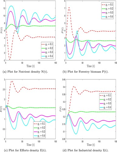
Numerical simulations are presented to study the dynamic complexity of compartments of the proposed time-fractional order forestry biomass system. Our analysis used the Adams-Bashforth technique along with Caputo-Fabrizio and F-F Caputo operators. To demonstrate the effectiveness of the suggested strategy, simulations were performed using MATLAB [32]. Table 1 shows the parameter values used for simulations derived from the literature. Fractional derivatives and fractal dimensions in time can be used to examine various intrinsic properties of the forestry biomass model, compared to classical order $\psi =1$ models. As a first step, we simulate different fractional order values with fixed parameter values. As a next step, we investigate the effects of changing the sensitive parameter values. Considering different values of fractional order, it is crucial to investigate the impact of these key parameters on solution profiles for crucial decisions.

Table 1. Displays the parameter values in the following manner.

Parameters	Numerical values	Description
Q	4	Constant input rate of nutrients
β	0.7	Utilization rate of nutrients by forestry biomass
$d_1$	0.3	Washout rate of nutrients
r	0.2	Modified intrinsic growth rate of forestry biomass
$r_0$	0.01	Constant
K	70	Carrying capacity of forestry biomass
$q_1$	0.2	Harvesting rate of forestry biomass
γ	0.1	New plantation rate
$d_2$	0.03	Illegal logging of forestry biomass
p	0.35	Fixed price unit of forestry biomass
τ	0.25	Tax per unit of forestry biomass
c	0.08	Fixed cost per unit of effort expanded to harvest forestry biomass
α	0.03	Constant
μ	0.1	Maximum growth due to alternative industries
$d_3$	0.3	Reduction rate of industries

Figure 2 shows the three-dimensional dynamic behaviour of the forestry biomass model (31(31) $\begin{array}{rl}{}^{\mathrm{FFP}}{}_{0+}{\mathfrak{D}}_t^{\psi ,\phi }N\left(t\right)& =Q-\text{β}P-d_{1}N,\\ {}^{\mathrm{FFP}}{}_{0+}{\mathfrak{D}}_t^{\psi ,\phi }P\left(t\right)& =r\left(N\right)P(1-\frac{P}{K})-q_1\mathrm{PE}-d_2\mathrm{PE}+\mathrm{\gamma P},\\ {}^{\mathrm{FFP}}{}_{0+}{\mathfrak{D}}_t^{\psi ,\phi }E\left(t\right)& =q_1(p-\tau )\mathrm{PE}+p{d}_2\mathrm{PE}-\mathrm{cE},\\ {}^{\mathrm{FFP}}{}_{0+}{\mathfrak{D}}_t^{\psi ,\phi }I\left(t\right)& =\mathrm{\alpha E}+\mathrm{\mu I}(1-\frac{P}{K})-d_{3}I.\end{array}$(31) ) at different fractional orders and fractal dimensions using F-F Caputo derivative. Figure 3 illustrates the two-dimensional dynamic behaviour of the forestry biomass model (31(31) $\begin{array}{rl}{}^{\mathrm{FFP}}{}_{0+}{\mathfrak{D}}_t^{\psi ,\phi }N\left(t\right)& =Q-\text{β}P-d_{1}N,\\ {}^{\mathrm{FFP}}{}_{0+}{\mathfrak{D}}_t^{\psi ,\phi }P\left(t\right)& =r\left(N\right)P(1-\frac{P}{K})-q_1\mathrm{PE}-d_2\mathrm{PE}+\mathrm{\gamma P},\\ {}^{\mathrm{FFP}}{}_{0+}{\mathfrak{D}}_t^{\psi ,\phi }E\left(t\right)& =q_1(p-\tau )\mathrm{PE}+p{d}_2\mathrm{PE}-\mathrm{cE},\\ {}^{\mathrm{FFP}}{}_{0+}{\mathfrak{D}}_t^{\psi ,\phi }I\left(t\right)& =\mathrm{\alpha E}+\mathrm{\mu I}(1-\frac{P}{K})-d_{3}I.\end{array}$(31) ) at different fractional orders and fractal dimensions using F-F Caputo derivative. Figure 4 represents the time series plots of the forestry biomass model (31(31) $\begin{array}{rl}{}^{\mathrm{FFP}}{}_{0+}{\mathfrak{D}}_t^{\psi ,\phi }N\left(t\right)& =Q-\text{β}P-d_{1}N,\\ {}^{\mathrm{FFP}}{}_{0+}{\mathfrak{D}}_t^{\psi ,\phi }P\left(t\right)& =r\left(N\right)P(1-\frac{P}{K})-q_1\mathrm{PE}-d_2\mathrm{PE}+\mathrm{\gamma P},\\ {}^{\mathrm{FFP}}{}_{0+}{\mathfrak{D}}_t^{\psi ,\phi }E\left(t\right)& =q_1(p-\tau )\mathrm{PE}+p{d}_2\mathrm{PE}-\mathrm{cE},\\ {}^{\mathrm{FFP}}{}_{0+}{\mathfrak{D}}_t^{\psi ,\phi }I\left(t\right)& =\mathrm{\alpha E}+\mathrm{\mu I}(1-\frac{P}{K})-d_{3}I.\end{array}$(31) ) at different fractional orders and fractal dimensions using F-F Caputo derivative. We observed that the nutrient density fluctuated at varied rates for combinations of ψ and φ before reaching a stable equilibrium point during the simulation. In contrast, the forestry biomass showed a quick drop, a rise, and a slow reduction for different fractional orders and dimensions. Similar trends were seen in the effort intensity measure, which rose and fell over time on varying pathways depending on the fractional orders. The industrial density increases quickly and then stabilizes after some time. Further, when the fractal dimension is fixed $\phi =1$, then we have analysed the behaviour of all state variables of proposed model. So, Figure 5 shows the three-dimensional dynamic behaviour of the forestry biomass model (31(31) $\begin{array}{rl}{}^{\mathrm{FFP}}{}_{0+}{\mathfrak{D}}_t^{\psi ,\phi }N\left(t\right)& =Q-\text{β}P-d_{1}N,\\ {}^{\mathrm{FFP}}{}_{0+}{\mathfrak{D}}_t^{\psi ,\phi }P\left(t\right)& =r\left(N\right)P(1-\frac{P}{K})-q_1\mathrm{PE}-d_2\mathrm{PE}+\mathrm{\gamma P},\\ {}^{\mathrm{FFP}}{}_{0+}{\mathfrak{D}}_t^{\psi ,\phi }E\left(t\right)& =q_1(p-\tau )\mathrm{PE}+p{d}_2\mathrm{PE}-\mathrm{cE},\\ {}^{\mathrm{FFP}}{}_{0+}{\mathfrak{D}}_t^{\psi ,\phi }I\left(t\right)& =\mathrm{\alpha E}+\mathrm{\mu I}(1-\frac{P}{K})-d_{3}I.\end{array}$(31) ) at different fractional orders. Figure 6 illustrates the two-dimensional dynamic behaviour of the forestry biomass model (31(31) $\begin{array}{rl}{}^{\mathrm{FFP}}{}_{0+}{\mathfrak{D}}_t^{\psi ,\phi }N\left(t\right)& =Q-\text{β}P-d_{1}N,\\ {}^{\mathrm{FFP}}{}_{0+}{\mathfrak{D}}_t^{\psi ,\phi }P\left(t\right)& =r\left(N\right)P(1-\frac{P}{K})-q_1\mathrm{PE}-d_2\mathrm{PE}+\mathrm{\gamma P},\\ {}^{\mathrm{FFP}}{}_{0+}{\mathfrak{D}}_t^{\psi ,\phi }E\left(t\right)& =q_1(p-\tau )\mathrm{PE}+p{d}_2\mathrm{PE}-\mathrm{cE},\\ {}^{\mathrm{FFP}}{}_{0+}{\mathfrak{D}}_t^{\psi ,\phi }I\left(t\right)& =\mathrm{\alpha E}+\mathrm{\mu I}(1-\frac{P}{K})-d_{3}I.\end{array}$(31) ) at different fractional orders. Figure 7 represents the time series plots of the forestry biomass model (31(31) $\begin{array}{rl}{}^{\mathrm{FFP}}{}_{0+}{\mathfrak{D}}_t^{\psi ,\phi }N\left(t\right)& =Q-\text{β}P-d_{1}N,\\ {}^{\mathrm{FFP}}{}_{0+}{\mathfrak{D}}_t^{\psi ,\phi }P\left(t\right)& =r\left(N\right)P(1-\frac{P}{K})-q_1\mathrm{PE}-d_2\mathrm{PE}+\mathrm{\gamma P},\\ {}^{\mathrm{FFP}}{}_{0+}{\mathfrak{D}}_t^{\psi ,\phi }E\left(t\right)& =q_1(p-\tau )\mathrm{PE}+p{d}_2\mathrm{PE}-\mathrm{cE},\\ {}^{\mathrm{FFP}}{}_{0+}{\mathfrak{D}}_t^{\psi ,\phi }I\left(t\right)& =\mathrm{\alpha E}+\mathrm{\mu I}(1-\frac{P}{K})-d_{3}I.\end{array}$(31) ) at different fractional orders. Additionally, as observed in this figure, the proposed model becomes rapidly stable when the fractional order ψ is changed compared to the integer model. Figure 8 exhibits the time series diagrams of the forestry biomass model (31(31) $\begin{array}{rl}{}^{\mathrm{FFP}}{}_{0+}{\mathfrak{D}}_t^{\psi ,\phi }N\left(t\right)& =Q-\text{β}P-d_{1}N,\\ {}^{\mathrm{FFP}}{}_{0+}{\mathfrak{D}}_t^{\psi ,\phi }P\left(t\right)& =r\left(N\right)P(1-\frac{P}{K})-q_1\mathrm{PE}-d_2\mathrm{PE}+\mathrm{\gamma P},\\ {}^{\mathrm{FFP}}{}_{0+}{\mathfrak{D}}_t^{\psi ,\phi }E\left(t\right)& =q_1(p-\tau )\mathrm{PE}+p{d}_2\mathrm{PE}-\mathrm{cE},\\ {}^{\mathrm{FFP}}{}_{0+}{\mathfrak{D}}_t^{\psi ,\phi }I\left(t\right)& =\mathrm{\alpha E}+\mathrm{\mu I}(1-\frac{P}{K})-d_{3}I.\end{array}$(31) ) at different fractal dimension orders and fractional order is fixed $\psi =1$. Next, we analysed the forestry biomass model with the Caputo-Fabrizio derivative. Figure 9 shows the three-dimensional dynamic behaviour of the forestry biomass model (6(6) $\begin{array}{rl}{}^{\mathrm{FFE}}{}_{0+}{\mathfrak{D}}_t^{\psi ,\phi }N\left(t\right)& =Q-\text{β}P-d_{1}N,\\ {}^{\mathrm{FFE}}{}_{0+}{\mathfrak{D}}_t^{\psi ,\phi }P\left(t\right)& =r\left(N\right)P(1-\frac{P}{K})-q_1\mathrm{PE}-d_2\mathrm{PE}+\mathrm{\gamma P},\\ {}^{\mathrm{FFE}}{}_{0+}{\mathfrak{D}}_t^{\psi ,\phi }E\left(t\right)& =q_1(p-\tau )\mathrm{PE}+p{d}_2\mathrm{PE}-\mathrm{cE},\\ {}^{\mathrm{FFE}}{}_{0+}{\mathfrak{D}}_t^{\psi ,\phi }I\left(t\right)& =\mathrm{\alpha E}+\mathrm{\mu I}(1-\frac{P}{K})-d_{3}I,\end{array}$(6) ) at different fractional orders using Caputo-Fabrizio derivative. Figure 10 illustrates the two-dimensional dynamic behaviour of the forestry biomass model (6(6) $\begin{array}{rl}{}^{\mathrm{FFE}}{}_{0+}{\mathfrak{D}}_t^{\psi ,\phi }N\left(t\right)& =Q-\text{β}P-d_{1}N,\\ {}^{\mathrm{FFE}}{}_{0+}{\mathfrak{D}}_t^{\psi ,\phi }P\left(t\right)& =r\left(N\right)P(1-\frac{P}{K})-q_1\mathrm{PE}-d_2\mathrm{PE}+\mathrm{\gamma P},\\ {}^{\mathrm{FFE}}{}_{0+}{\mathfrak{D}}_t^{\psi ,\phi }E\left(t\right)& =q_1(p-\tau )\mathrm{PE}+p{d}_2\mathrm{PE}-\mathrm{cE},\\ {}^{\mathrm{FFE}}{}_{0+}{\mathfrak{D}}_t^{\psi ,\phi }I\left(t\right)& =\mathrm{\alpha E}+\mathrm{\mu I}(1-\frac{P}{K})-d_{3}I,\end{array}$(6) ) at different fractional orders using Caputo-Fabrizio derivative. Figure 11 represents the time series plots of the forestry biomass model (6(6) $\begin{array}{rl}{}^{\mathrm{FFE}}{}_{0+}{\mathfrak{D}}_t^{\psi ,\phi }N\left(t\right)& =Q-\text{β}P-d_{1}N,\\ {}^{\mathrm{FFE}}{}_{0+}{\mathfrak{D}}_t^{\psi ,\phi }P\left(t\right)& =r\left(N\right)P(1-\frac{P}{K})-q_1\mathrm{PE}-d_2\mathrm{PE}+\mathrm{\gamma P},\\ {}^{\mathrm{FFE}}{}_{0+}{\mathfrak{D}}_t^{\psi ,\phi }E\left(t\right)& =q_1(p-\tau )\mathrm{PE}+p{d}_2\mathrm{PE}-\mathrm{cE},\\ {}^{\mathrm{FFE}}{}_{0+}{\mathfrak{D}}_t^{\psi ,\phi }I\left(t\right)& =\mathrm{\alpha E}+\mathrm{\mu I}(1-\frac{P}{K})-d_{3}I,\end{array}$(6) ) at different fractional orders using Caputo-Fabrizio derivative. Because even a tiny adjustment to the sensitive parameter will result in a significant change, it is essential to estimate extremely delicate parameters correctly. Adjusting a less sensitive parameter won't significantly impact the system's behaviour and will take time to calculate. The investigation has led us to the sensitive factors, $d_2$ and $q_1$. Moreover, we analysed the dynamic complexity of the different parameter values. So, Figure 12 exhibits 3D dynamic behaviour of the forestry biomass model (31(31) $\begin{array}{rl}{}^{\mathrm{FFP}}{}_{0+}{\mathfrak{D}}_t^{\psi ,\phi }N\left(t\right)& =Q-\text{β}P-d_{1}N,\\ {}^{\mathrm{FFP}}{}_{0+}{\mathfrak{D}}_t^{\psi ,\phi }P\left(t\right)& =r\left(N\right)P(1-\frac{P}{K})-q_1\mathrm{PE}-d_2\mathrm{PE}+\mathrm{\gamma P},\\ {}^{\mathrm{FFP}}{}_{0+}{\mathfrak{D}}_t^{\psi ,\phi }E\left(t\right)& =q_1(p-\tau )\mathrm{PE}+p{d}_2\mathrm{PE}-\mathrm{cE},\\ {}^{\mathrm{FFP}}{}_{0+}{\mathfrak{D}}_t^{\psi ,\phi }I\left(t\right)& =\mathrm{\alpha E}+\mathrm{\mu I}(1-\frac{P}{K})-d_{3}I.\end{array}$(31) ) at different illegal logging of forestry biomass $d_2=0.03,0.06,0.12,0.24$. Figure 13 illustrates the 2D dynamic behaviour of the forestry biomass model (31(31) $\begin{array}{rl}{}^{\mathrm{FFP}}{}_{0+}{\mathfrak{D}}_t^{\psi ,\phi }N\left(t\right)& =Q-\text{β}P-d_{1}N,\\ {}^{\mathrm{FFP}}{}_{0+}{\mathfrak{D}}_t^{\psi ,\phi }P\left(t\right)& =r\left(N\right)P(1-\frac{P}{K})-q_1\mathrm{PE}-d_2\mathrm{PE}+\mathrm{\gamma P},\\ {}^{\mathrm{FFP}}{}_{0+}{\mathfrak{D}}_t^{\psi ,\phi }E\left(t\right)& =q_1(p-\tau )\mathrm{PE}+p{d}_2\mathrm{PE}-\mathrm{cE},\\ {}^{\mathrm{FFP}}{}_{0+}{\mathfrak{D}}_t^{\psi ,\phi }I\left(t\right)& =\mathrm{\alpha E}+\mathrm{\mu I}(1-\frac{P}{K})-d_{3}I.\end{array}$(31) ) at different illegal logging of forestry biomass $d_2=0.03,0.06,0.12,\mathrm{0.24.}$ Figure 14 represents the time series plots of the forestry biomass model (31(31) $\begin{array}{rl}{}^{\mathrm{FFP}}{}_{0+}{\mathfrak{D}}_t^{\psi ,\phi }N\left(t\right)& =Q-\text{β}P-d_{1}N,\\ {}^{\mathrm{FFP}}{}_{0+}{\mathfrak{D}}_t^{\psi ,\phi }P\left(t\right)& =r\left(N\right)P(1-\frac{P}{K})-q_1\mathrm{PE}-d_2\mathrm{PE}+\mathrm{\gamma P},\\ {}^{\mathrm{FFP}}{}_{0+}{\mathfrak{D}}_t^{\psi ,\phi }E\left(t\right)& =q_1(p-\tau )\mathrm{PE}+p{d}_2\mathrm{PE}-\mathrm{cE},\\ {}^{\mathrm{FFP}}{}_{0+}{\mathfrak{D}}_t^{\psi ,\phi }I\left(t\right)& =\mathrm{\alpha E}+\mathrm{\mu I}(1-\frac{P}{K})-d_{3}I.\end{array}$(31) ) at different illegal logging of forestry biomass $d_2=0.03,0.06,0.12,0.24$. A decline in forestry biomass is observed when the rate of illegal logging increases; this relationship is illustrated in Figure 14. Figure 15 exhibits 3D dynamic behaviour of the forestry biomass model (31(31) $\begin{array}{rl}{}^{\mathrm{FFP}}{}_{0+}{\mathfrak{D}}_t^{\psi ,\phi }N\left(t\right)& =Q-\text{β}P-d_{1}N,\\ {}^{\mathrm{FFP}}{}_{0+}{\mathfrak{D}}_t^{\psi ,\phi }P\left(t\right)& =r\left(N\right)P(1-\frac{P}{K})-q_1\mathrm{PE}-d_2\mathrm{PE}+\mathrm{\gamma P},\\ {}^{\mathrm{FFP}}{}_{0+}{\mathfrak{D}}_t^{\psi ,\phi }E\left(t\right)& =q_1(p-\tau )\mathrm{PE}+p{d}_2\mathrm{PE}-\mathrm{cE},\\ {}^{\mathrm{FFP}}{}_{0+}{\mathfrak{D}}_t^{\psi ,\phi }I\left(t\right)& =\mathrm{\alpha E}+\mathrm{\mu I}(1-\frac{P}{K})-d_{3}I.\end{array}$(31) ) at different harvesting rate of forestry biomass $q_1=0.1,0.2,0.3,0.4$. Figure 16 illustrates the 2D dynamic behaviour of the forestry biomass model (31(31) $\begin{array}{rl}{}^{\mathrm{FFP}}{}_{0+}{\mathfrak{D}}_t^{\psi ,\phi }N\left(t\right)& =Q-\text{β}P-d_{1}N,\\ {}^{\mathrm{FFP}}{}_{0+}{\mathfrak{D}}_t^{\psi ,\phi }P\left(t\right)& =r\left(N\right)P(1-\frac{P}{K})-q_1\mathrm{PE}-d_2\mathrm{PE}+\mathrm{\gamma P},\\ {}^{\mathrm{FFP}}{}_{0+}{\mathfrak{D}}_t^{\psi ,\phi }E\left(t\right)& =q_1(p-\tau )\mathrm{PE}+p{d}_2\mathrm{PE}-\mathrm{cE},\\ {}^{\mathrm{FFP}}{}_{0+}{\mathfrak{D}}_t^{\psi ,\phi }I\left(t\right)& =\mathrm{\alpha E}+\mathrm{\mu I}(1-\frac{P}{K})-d_{3}I.\end{array}$(31) ) at different harvesting rate of forestry biomass $q_1=0.1,0.2,0.3,0.4$ Figure 17 represents the time series plots of the forestry biomass model (31(31) $\begin{array}{rl}{}^{\mathrm{FFP}}{}_{0+}{\mathfrak{D}}_t^{\psi ,\phi }N\left(t\right)& =Q-\text{β}P-d_{1}N,\\ {}^{\mathrm{FFP}}{}_{0+}{\mathfrak{D}}_t^{\psi ,\phi }P\left(t\right)& =r\left(N\right)P(1-\frac{P}{K})-q_1\mathrm{PE}-d_2\mathrm{PE}+\mathrm{\gamma P},\\ {}^{\mathrm{FFP}}{}_{0+}{\mathfrak{D}}_t^{\psi ,\phi }E\left(t\right)& =q_1(p-\tau )\mathrm{PE}+p{d}_2\mathrm{PE}-\mathrm{cE},\\ {}^{\mathrm{FFP}}{}_{0+}{\mathfrak{D}}_t^{\psi ,\phi }I\left(t\right)& =\mathrm{\alpha E}+\mathrm{\mu I}(1-\frac{P}{K})-d_{3}I.\end{array}$(31) ) at different harvesting rate of forestry biomass $q_1=0.1,0.2,0.3,0.4$. A decline in forestry biomass is observed when the rate of harvesting increases; this relationship is illustrated in Figure 17.

Figure 2. Numerical simulation of forestry biomass model (31(31) $\begin{array}{rl}{}^{\mathrm{FFP}}{}_{0+}{\mathfrak{D}}_t^{\psi ,\phi }N\left(t\right)& =Q-\text{β}P-d_{1}N,\\ {}^{\mathrm{FFP}}{}_{0+}{\mathfrak{D}}_t^{\psi ,\phi }P\left(t\right)& =r\left(N\right)P(1-\frac{P}{K})-q_1\mathrm{PE}-d_2\mathrm{PE}+\mathrm{\gamma P},\\ {}^{\mathrm{FFP}}{}_{0+}{\mathfrak{D}}_t^{\psi ,\phi }E\left(t\right)& =q_1(p-\tau )\mathrm{PE}+p{d}_2\mathrm{PE}-\mathrm{cE},\\ {}^{\mathrm{FFP}}{}_{0+}{\mathfrak{D}}_t^{\psi ,\phi }I\left(t\right)& =\mathrm{\alpha E}+\mathrm{\mu I}(1-\frac{P}{K})-d_{3}I.\end{array}$(31) ) at arbitrary values of ψ and φ. (a) Plot for Nutrient density N(t). (b) Plot for Forestry biomass P(t). (c) Plot for Efforts density E(t) and (d) Plot for Industrial density I(t).

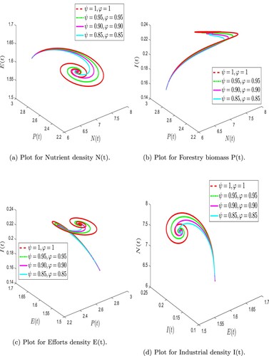
Figure 3. Numerical simulation of forestry biomass model (31(31) $\begin{array}{rl}{}^{\mathrm{FFP}}{}_{0+}{\mathfrak{D}}_t^{\psi ,\phi }N\left(t\right)& =Q-\text{β}P-d_{1}N,\\ {}^{\mathrm{FFP}}{}_{0+}{\mathfrak{D}}_t^{\psi ,\phi }P\left(t\right)& =r\left(N\right)P(1-\frac{P}{K})-q_1\mathrm{PE}-d_2\mathrm{PE}+\mathrm{\gamma P},\\ {}^{\mathrm{FFP}}{}_{0+}{\mathfrak{D}}_t^{\psi ,\phi }E\left(t\right)& =q_1(p-\tau )\mathrm{PE}+p{d}_2\mathrm{PE}-\mathrm{cE},\\ {}^{\mathrm{FFP}}{}_{0+}{\mathfrak{D}}_t^{\psi ,\phi }I\left(t\right)& =\mathrm{\alpha E}+\mathrm{\mu I}(1-\frac{P}{K})-d_{3}I.\end{array}$(31) ) at arbitrary values of ψ and φ. (a) Plot for Nutrient density N(t). (b) Plot for Forestry biomass P(t). (c) Plot for Efforts density E(t) and (d) Plot for Industrial density I(t).

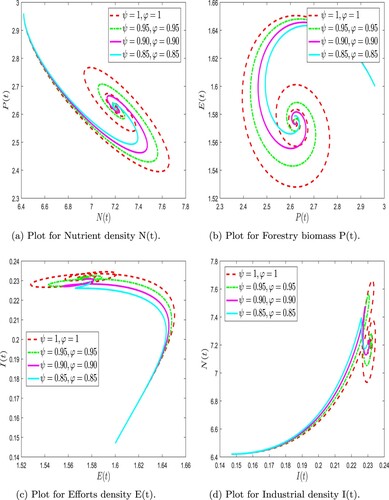
Figure 4. Numerical simulation of forestry biomass model (31(31) $\begin{array}{rl}{}^{\mathrm{FFP}}{}_{0+}{\mathfrak{D}}_t^{\psi ,\phi }N\left(t\right)& =Q-\text{β}P-d_{1}N,\\ {}^{\mathrm{FFP}}{}_{0+}{\mathfrak{D}}_t^{\psi ,\phi }P\left(t\right)& =r\left(N\right)P(1-\frac{P}{K})-q_1\mathrm{PE}-d_2\mathrm{PE}+\mathrm{\gamma P},\\ {}^{\mathrm{FFP}}{}_{0+}{\mathfrak{D}}_t^{\psi ,\phi }E\left(t\right)& =q_1(p-\tau )\mathrm{PE}+p{d}_2\mathrm{PE}-\mathrm{cE},\\ {}^{\mathrm{FFP}}{}_{0+}{\mathfrak{D}}_t^{\psi ,\phi }I\left(t\right)& =\mathrm{\alpha E}+\mathrm{\mu I}(1-\frac{P}{K})-d_{3}I.\end{array}$(31) ) at arbitrary values of ψ and φ. (a) Plot for Nutrient density N(t). (b) Plot for Forestry biomass P(t). (c) Plot for Efforts density E(t) and (d) Plot for Industrial density I(t).

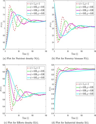
Figure 5. Numerical simulation of forestry biomass model (31(31) $\begin{array}{rl}{}^{\mathrm{FFP}}{}_{0+}{\mathfrak{D}}_t^{\psi ,\phi }N\left(t\right)& =Q-\text{β}P-d_{1}N,\\ {}^{\mathrm{FFP}}{}_{0+}{\mathfrak{D}}_t^{\psi ,\phi }P\left(t\right)& =r\left(N\right)P(1-\frac{P}{K})-q_1\mathrm{PE}-d_2\mathrm{PE}+\mathrm{\gamma P},\\ {}^{\mathrm{FFP}}{}_{0+}{\mathfrak{D}}_t^{\psi ,\phi }E\left(t\right)& =q_1(p-\tau )\mathrm{PE}+p{d}_2\mathrm{PE}-\mathrm{cE},\\ {}^{\mathrm{FFP}}{}_{0+}{\mathfrak{D}}_t^{\psi ,\phi }I\left(t\right)& =\mathrm{\alpha E}+\mathrm{\mu I}(1-\frac{P}{K})-d_{3}I.\end{array}$(31) ) at arbitrary values of ψ and fixed $\phi =1$. (a) Plot for Nutrient density N(t). (b) Plot for Forestry biomass P(t). (c) Plot for Efforts density E(t) and (d) Plot for Industrial density I(t).

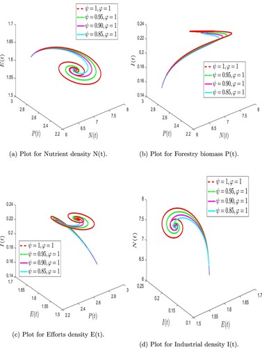
Figure 6. Numerical simulation of forestry biomass model (31(31) $\begin{array}{rl}{}^{\mathrm{FFP}}{}_{0+}{\mathfrak{D}}_t^{\psi ,\phi }N\left(t\right)& =Q-\text{β}P-d_{1}N,\\ {}^{\mathrm{FFP}}{}_{0+}{\mathfrak{D}}_t^{\psi ,\phi }P\left(t\right)& =r\left(N\right)P(1-\frac{P}{K})-q_1\mathrm{PE}-d_2\mathrm{PE}+\mathrm{\gamma P},\\ {}^{\mathrm{FFP}}{}_{0+}{\mathfrak{D}}_t^{\psi ,\phi }E\left(t\right)& =q_1(p-\tau )\mathrm{PE}+p{d}_2\mathrm{PE}-\mathrm{cE},\\ {}^{\mathrm{FFP}}{}_{0+}{\mathfrak{D}}_t^{\psi ,\phi }I\left(t\right)& =\mathrm{\alpha E}+\mathrm{\mu I}(1-\frac{P}{K})-d_{3}I.\end{array}$(31) ) at arbitrary values of ψ and fixed $\phi =1$. (a) Plot for Nutrient density N(t). (b) Plot for Forestry biomass P(t). (c)Plot for Efforts density E(t) and (d)Plot for Industrial density I(t).

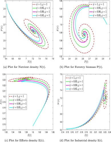
Figure 7. Numerical simulation of forestry biomass model (31(31) $\begin{array}{rl}{}^{\mathrm{FFP}}{}_{0+}{\mathfrak{D}}_t^{\psi ,\phi }N\left(t\right)& =Q-\text{β}P-d_{1}N,\\ {}^{\mathrm{FFP}}{}_{0+}{\mathfrak{D}}_t^{\psi ,\phi }P\left(t\right)& =r\left(N\right)P(1-\frac{P}{K})-q_1\mathrm{PE}-d_2\mathrm{PE}+\mathrm{\gamma P},\\ {}^{\mathrm{FFP}}{}_{0+}{\mathfrak{D}}_t^{\psi ,\phi }E\left(t\right)& =q_1(p-\tau )\mathrm{PE}+p{d}_2\mathrm{PE}-\mathrm{cE},\\ {}^{\mathrm{FFP}}{}_{0+}{\mathfrak{D}}_t^{\psi ,\phi }I\left(t\right)& =\mathrm{\alpha E}+\mathrm{\mu I}(1-\frac{P}{K})-d_{3}I.\end{array}$(31) ) at arbitrary values of ψ and fixed $\phi =1$. (a) Plot for Nutrient density N(t). (b) Plot for Forestry biomass P(t). (c) Plot for Efforts density E(t) and (d) Plot for Industrial density I(t).

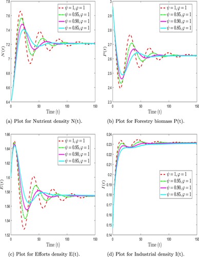
Figure 8. Numerical simulation of forestry biomass model (31(31) $\begin{array}{rl}{}^{\mathrm{FFP}}{}_{0+}{\mathfrak{D}}_t^{\psi ,\phi }N\left(t\right)& =Q-\text{β}P-d_{1}N,\\ {}^{\mathrm{FFP}}{}_{0+}{\mathfrak{D}}_t^{\psi ,\phi }P\left(t\right)& =r\left(N\right)P(1-\frac{P}{K})-q_1\mathrm{PE}-d_2\mathrm{PE}+\mathrm{\gamma P},\\ {}^{\mathrm{FFP}}{}_{0+}{\mathfrak{D}}_t^{\psi ,\phi }E\left(t\right)& =q_1(p-\tau )\mathrm{PE}+p{d}_2\mathrm{PE}-\mathrm{cE},\\ {}^{\mathrm{FFP}}{}_{0+}{\mathfrak{D}}_t^{\psi ,\phi }I\left(t\right)& =\mathrm{\alpha E}+\mathrm{\mu I}(1-\frac{P}{K})-d_{3}I.\end{array}$(31) ) at arbitrary values of φ and fixed $\psi =1$. (a) Plot for Nutrient density N(t). (b) Plot for Forestry biomass P(t). (c) Plot for Efforts density E(t) and (d) Plot for Industrial density I(t).

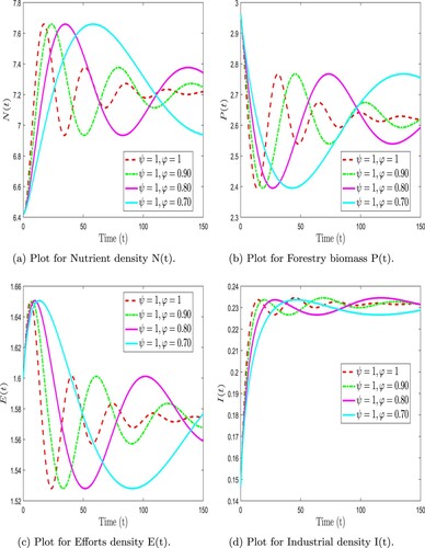
Figure 9. Numerical simulation of forestry biomass model (6(6) $\begin{array}{rl}{}^{\mathrm{FFE}}{}_{0+}{\mathfrak{D}}_t^{\psi ,\phi }N\left(t\right)& =Q-\text{β}P-d_{1}N,\\ {}^{\mathrm{FFE}}{}_{0+}{\mathfrak{D}}_t^{\psi ,\phi }P\left(t\right)& =r\left(N\right)P(1-\frac{P}{K})-q_1\mathrm{PE}-d_2\mathrm{PE}+\mathrm{\gamma P},\\ {}^{\mathrm{FFE}}{}_{0+}{\mathfrak{D}}_t^{\psi ,\phi }E\left(t\right)& =q_1(p-\tau )\mathrm{PE}+p{d}_2\mathrm{PE}-\mathrm{cE},\\ {}^{\mathrm{FFE}}{}_{0+}{\mathfrak{D}}_t^{\psi ,\phi }I\left(t\right)& =\mathrm{\alpha E}+\mathrm{\mu I}(1-\frac{P}{K})-d_{3}I,\end{array}$(6) ) at arbitrary values of ψ. (a) Plot for Nutrient density N(t). (b) Plot for Forestry biomass P(t). (c) Plot for Efforts density E(t) and (d) Plot for Industrial density I(t).

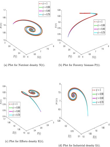
Figure 10. Numerical simulation of forestry biomass model (6(6) $\begin{array}{rl}{}^{\mathrm{FFE}}{}_{0+}{\mathfrak{D}}_t^{\psi ,\phi }N\left(t\right)& =Q-\text{β}P-d_{1}N,\\ {}^{\mathrm{FFE}}{}_{0+}{\mathfrak{D}}_t^{\psi ,\phi }P\left(t\right)& =r\left(N\right)P(1-\frac{P}{K})-q_1\mathrm{PE}-d_2\mathrm{PE}+\mathrm{\gamma P},\\ {}^{\mathrm{FFE}}{}_{0+}{\mathfrak{D}}_t^{\psi ,\phi }E\left(t\right)& =q_1(p-\tau )\mathrm{PE}+p{d}_2\mathrm{PE}-\mathrm{cE},\\ {}^{\mathrm{FFE}}{}_{0+}{\mathfrak{D}}_t^{\psi ,\phi }I\left(t\right)& =\mathrm{\alpha E}+\mathrm{\mu I}(1-\frac{P}{K})-d_{3}I,\end{array}$(6) ) at arbitrary values of ψ. (a) Plot for Nutrient density N(t). (b) Plot for Forestry biomass P(t). (c) Plot for Efforts density E(t) and (d) Plot for Industrial density I(t).

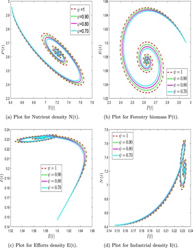
Figure 11. Numerical simulation of forestry biomass model (6(6) $\begin{array}{rl}{}^{\mathrm{FFE}}{}_{0+}{\mathfrak{D}}_t^{\psi ,\phi }N\left(t\right)& =Q-\text{β}P-d_{1}N,\\ {}^{\mathrm{FFE}}{}_{0+}{\mathfrak{D}}_t^{\psi ,\phi }P\left(t\right)& =r\left(N\right)P(1-\frac{P}{K})-q_1\mathrm{PE}-d_2\mathrm{PE}+\mathrm{\gamma P},\\ {}^{\mathrm{FFE}}{}_{0+}{\mathfrak{D}}_t^{\psi ,\phi }E\left(t\right)& =q_1(p-\tau )\mathrm{PE}+p{d}_2\mathrm{PE}-\mathrm{cE},\\ {}^{\mathrm{FFE}}{}_{0+}{\mathfrak{D}}_t^{\psi ,\phi }I\left(t\right)& =\mathrm{\alpha E}+\mathrm{\mu I}(1-\frac{P}{K})-d_{3}I,\end{array}$(6) ) at arbitrary values of ψ. (a) Plot for Nutrient density N(t). (b) Plot for Forestry biomass P(t). (c) Plot for Efforts density E(t) and (d) Plot for Industrial density I(t).

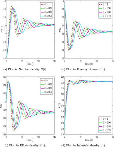
Figure 12. Numerical simulation of forestry biomass model (31(31) $\begin{array}{rl}{}^{\mathrm{FFP}}{}_{0+}{\mathfrak{D}}_t^{\psi ,\phi }N\left(t\right)& =Q-\text{β}P-d_{1}N,\\ {}^{\mathrm{FFP}}{}_{0+}{\mathfrak{D}}_t^{\psi ,\phi }P\left(t\right)& =r\left(N\right)P(1-\frac{P}{K})-q_1\mathrm{PE}-d_2\mathrm{PE}+\mathrm{\gamma P},\\ {}^{\mathrm{FFP}}{}_{0+}{\mathfrak{D}}_t^{\psi ,\phi }E\left(t\right)& =q_1(p-\tau )\mathrm{PE}+p{d}_2\mathrm{PE}-\mathrm{cE},\\ {}^{\mathrm{FFP}}{}_{0+}{\mathfrak{D}}_t^{\psi ,\phi }I\left(t\right)& =\mathrm{\alpha E}+\mathrm{\mu I}(1-\frac{P}{K})-d_{3}I.\end{array}$(31) ) at arbitrary values of $d_2$ with $\psi =0.99$. (a) Plot for Nutrient density N(t). (b) Plot for Forestry biomass P(t). (c) Plot for Efforts density E(t) and (d) Plot for Industrial density I(t).

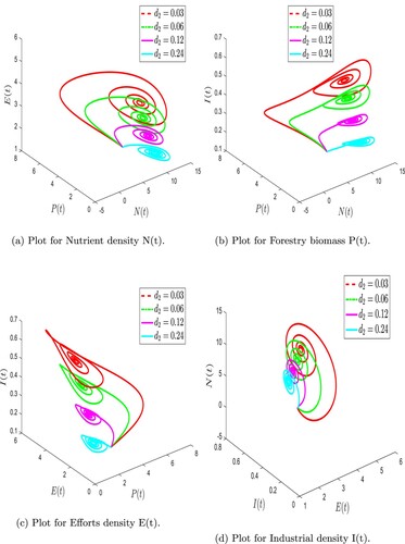
Figure 13. Numerical simulation of forestry biomass model (31(31) $\begin{array}{rl}{}^{\mathrm{FFP}}{}_{0+}{\mathfrak{D}}_t^{\psi ,\phi }N\left(t\right)& =Q-\text{β}P-d_{1}N,\\ {}^{\mathrm{FFP}}{}_{0+}{\mathfrak{D}}_t^{\psi ,\phi }P\left(t\right)& =r\left(N\right)P(1-\frac{P}{K})-q_1\mathrm{PE}-d_2\mathrm{PE}+\mathrm{\gamma P},\\ {}^{\mathrm{FFP}}{}_{0+}{\mathfrak{D}}_t^{\psi ,\phi }E\left(t\right)& =q_1(p-\tau )\mathrm{PE}+p{d}_2\mathrm{PE}-\mathrm{cE},\\ {}^{\mathrm{FFP}}{}_{0+}{\mathfrak{D}}_t^{\psi ,\phi }I\left(t\right)& =\mathrm{\alpha E}+\mathrm{\mu I}(1-\frac{P}{K})-d_{3}I.\end{array}$(31) ) at arbitrary values of $d_2$ with $\psi =0.99$. (a) Plot for Nutrient density N(t). (b) Plot for Forestry biomass P(t). (c) Plot for Efforts density E(t) and (d) Plot for Industrial density I(t).

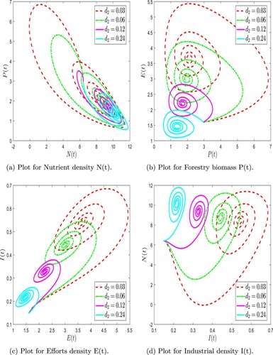
Figure 14. Numerical simulation of forestry biomass model (31(31) $\begin{array}{rl}{}^{\mathrm{FFP}}{}_{0+}{\mathfrak{D}}_t^{\psi ,\phi }N\left(t\right)& =Q-\text{β}P-d_{1}N,\\ {}^{\mathrm{FFP}}{}_{0+}{\mathfrak{D}}_t^{\psi ,\phi }P\left(t\right)& =r\left(N\right)P(1-\frac{P}{K})-q_1\mathrm{PE}-d_2\mathrm{PE}+\mathrm{\gamma P},\\ {}^{\mathrm{FFP}}{}_{0+}{\mathfrak{D}}_t^{\psi ,\phi }E\left(t\right)& =q_1(p-\tau )\mathrm{PE}+p{d}_2\mathrm{PE}-\mathrm{cE},\\ {}^{\mathrm{FFP}}{}_{0+}{\mathfrak{D}}_t^{\psi ,\phi }I\left(t\right)& =\mathrm{\alpha E}+\mathrm{\mu I}(1-\frac{P}{K})-d_{3}I.\end{array}$(31) ) at arbitrary values of $d_2$ with $\psi =0.99$. (a) Plot for Nutrient density N(t). (b) Plot for Forestry biomass P(t). (c) Plot for Efforts density E(t) and (d) Plot for Industrial density I(t).

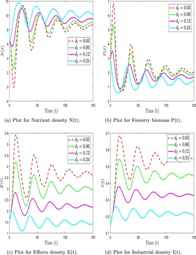
Figure 15. Numerical simulation of forestry biomass model (31(31) $\begin{array}{rl}{}^{\mathrm{FFP}}{}_{0+}{\mathfrak{D}}_t^{\psi ,\phi }N\left(t\right)& =Q-\text{β}P-d_{1}N,\\ {}^{\mathrm{FFP}}{}_{0+}{\mathfrak{D}}_t^{\psi ,\phi }P\left(t\right)& =r\left(N\right)P(1-\frac{P}{K})-q_1\mathrm{PE}-d_2\mathrm{PE}+\mathrm{\gamma P},\\ {}^{\mathrm{FFP}}{}_{0+}{\mathfrak{D}}_t^{\psi ,\phi }E\left(t\right)& =q_1(p-\tau )\mathrm{PE}+p{d}_2\mathrm{PE}-\mathrm{cE},\\ {}^{\mathrm{FFP}}{}_{0+}{\mathfrak{D}}_t^{\psi ,\phi }I\left(t\right)& =\mathrm{\alpha E}+\mathrm{\mu I}(1-\frac{P}{K})-d_{3}I.\end{array}$(31) ) at arbitrary values of $q_1$ with $\psi =0.99$. (a) Plot for Nutrient density N(t). (b) Plot for Forestry biomass P(t). (c) Plot for Efforts density E(t) and (d) Plot for Industrial density I(t).

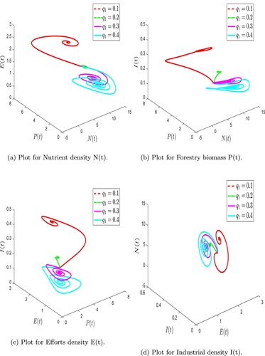
Figure 16. Numerical simulation of forestry biomass model (31(31) $\begin{array}{rl}{}^{\mathrm{FFP}}{}_{0+}{\mathfrak{D}}_t^{\psi ,\phi }N\left(t\right)& =Q-\text{β}P-d_{1}N,\\ {}^{\mathrm{FFP}}{}_{0+}{\mathfrak{D}}_t^{\psi ,\phi }P\left(t\right)& =r\left(N\right)P(1-\frac{P}{K})-q_1\mathrm{PE}-d_2\mathrm{PE}+\mathrm{\gamma P},\\ {}^{\mathrm{FFP}}{}_{0+}{\mathfrak{D}}_t^{\psi ,\phi }E\left(t\right)& =q_1(p-\tau )\mathrm{PE}+p{d}_2\mathrm{PE}-\mathrm{cE},\\ {}^{\mathrm{FFP}}{}_{0+}{\mathfrak{D}}_t^{\psi ,\phi }I\left(t\right)& =\mathrm{\alpha E}+\mathrm{\mu I}(1-\frac{P}{K})-d_{3}I.\end{array}$(31) ) at arbitrary values of $q_1$ with $\psi =0.99$. (a) Plot for Nutrient density N(t). (b) Plot for Forestry biomass P(t). (c) Plot for Efforts density E(t) and (d) Plot for Industrial density I(t).

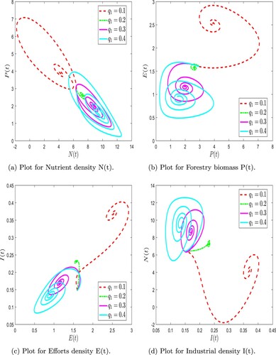
Figure 17. Numerical simulation of forestry biomass model (31(31) $\begin{array}{rl}{}^{\mathrm{FFP}}{}_{0+}{\mathfrak{D}}_t^{\psi ,\phi }N\left(t\right)& =Q-\text{β}P-d_{1}N,\\ {}^{\mathrm{FFP}}{}_{0+}{\mathfrak{D}}_t^{\psi ,\phi }P\left(t\right)& =r\left(N\right)P(1-\frac{P}{K})-q_1\mathrm{PE}-d_2\mathrm{PE}+\mathrm{\gamma P},\\ {}^{\mathrm{FFP}}{}_{0+}{\mathfrak{D}}_t^{\psi ,\phi }E\left(t\right)& =q_1(p-\tau )\mathrm{PE}+p{d}_2\mathrm{PE}-\mathrm{cE},\\ {}^{\mathrm{FFP}}{}_{0+}{\mathfrak{D}}_t^{\psi ,\phi }I\left(t\right)& =\mathrm{\alpha E}+\mathrm{\mu I}(1-\frac{P}{K})-d_{3}I.\end{array}$(31) ) at arbitrary values of $q_1$ with $\psi =0.99$. (a) Plot for Nutrient density N(t). (b) Plot for Forestry biomass P(t). (c) Plot for Efforts density E(t) and (d) Plot for Industrial density I(t).

7. Conclusion

In this research, we have demonstrated how illegal logging and tax imposition affect the utilization and preservation of forestry biomass. The proposed model study also assesses the impact of alternative resources on the development of industries. This research aims to analyse forestry biomass system dynamics utilizing effective approximation techniques for the F-F derivatives in the Caputo and C-F sense. Among the most fundamental features of these versions is the concept of memory. The F-F idea can predict the system complexity in two orders more precisely. First, we prove the existence and uniqueness of the fractional-order system and then the numerical solution of it through numerical simulation. The numerical analysis demonstrates that forestry biomass can be preserved more economically when government organizations implement the tax. Numerical simulations show more powerful converging effects of the forestry biomass model for different fractional orders resembling integer orders. The fractal fractional operator has been used in two senses to obtain the numerical results for the non-integer model presented here. The analysis shows that forestry biomass increases more quickly in the presence of tax $\left(\tau \right)$ than in the absence of tax. We identify sensitive parameters in the proposed model and analyse those to examine the behaviour of the numerical solution and its sensitivity to different transmission parameters. It has been shown that even a slight change in the order of derivatives and the system parameters can significantly influence the behaviour of a graphical representation. The techniques presented in this research can be extended along with other operators. In the future, it can be beneficial if we resolve the proposed model with the help of other different numerical techniques and compare the numerical solutions. Finding the best way for forestry biomass conservation and the optimal control policy applied.

Acknowledgement

Researchers Supporting Project number (RSPD2024R526), King Saud University, Riyadh, Saudi Arabia.

Authors contributions

All authors contributed equally and significantly in writing this paper and typed,read, and approved the final manuscript.

Disclosure statement

No potential conflict of interest was reported by the author(s).

Data availability statements

Data available on request from the authors.

References

- Hilfer R. Applications of fractional calculus in physics. Universität Mainz & Universität Stuttgart, Germany: World Scientific; 2000. p. 472. doi: 10.1142/3779
- Machado JT, Kiryakova V, Mainardi F. Recent history of fractional calculus. Commun Nonlinear Sci Numer Simul. 2011;16(3):1140–1153. doi: 10.1016/j.cnsns.2010.05.027
- Sabatier JATMJ, Agrawal OP, Machado JAT. Advances in fractional calculus. Vol. 4. Dordrecht: Springer; 2007. doi: 10.1007/978-1-4020-6042-7
- Das S. Functional fractional calculus. Vol. 1. Berlin Heidelberg: Springer-Verlag; 2011. doi: 10.1007/978-3-642-20545-3. ISBN 978-3-642-20544-6
- Atangana A, Araz S.I. New numerical approximation for chua attractor with fractional and fractal-fractional operators. Alex Eng J. 2020;59(5):3275–3296. doi: 10.1016/j.aej.2020.01.004
- Khan MA, Atangana A, Muhammad T, et al. Numerical solution of a fractal-fractional order chaotic circuit system. Rev Mex Fís. 2021;67(5):5. doi: 10.31349/RevMexFis.67.051401
- Atangana A. Fractal-fractional differentiation and integration: connecting fractal calculus and fractional calculus to predict complex system. Chaos Solitons Fract. 2017;102:396–406. doi: 10.1016/j.chaos.2017.04.027
- Wang W, Khan MA. Analysis and numerical simulation of fractional model of bank data with fractal–fractional atangana–baleanu derivative. J Comput Appl Math. 2020;369:112646. doi: 10.1016/j.cam.2019.112646
- Ghanbari B. On the modeling of the interaction between tumor growth and the immune system using some new fractional and fractional-fractal operators. Adv Differ Equ. 2020;2020(1):585. doi: 10.1186/s13662-020-03040-x
- Kumar P, Kumar A, Kumar S, et al. A fractional order co-infection model between malaria and filariasis epidemic. Arab J Basic Appl Sci. 2024;31(1):132–153.
- Khan MA. The dynamics of dengue infection through fractal-fractional operator with real statistical data. Alex Eng J. 2021;60(1):321–336. doi: 10.1016/j.aej.2020.08.018
- Diethelm K, Ford NJ, Freed AD. A predictor-corrector approach for the numerical solution of fractional differential equations. Nonlinear Dyn. 2002;29:3–22. doi: 10.1023/A:1016592219341
- Daftardar-Gejji V, Sukale Y, Bhalekar S. A new predictor–corrector method for fractional differential equations. Appl Math Comput. 2014;244:158–182.
- Ali Z, Rabiei F, Shah K, et al. Fractal-fractional order dynamical behavior of an hiv/aids epidemic mathematical model. Eur Phys J Plus. 2021;136(1):36. doi: 10.1140/epjp/s13360-020-00994-5
- Abro KA. Numerical study and chaotic oscillations for aerodynamic model of wind turbine via fractal and fractional differential operators. Numer Methods Partial Differ Equ. 2022;38(5):1180–1194. doi: 10.1002/num.v38.5
- Baleanu D, Diethelm K, Scalas E, et al. Fractional calculus: models and numerical methods. Vol. 3. Singapore: World Scientific; 2012. p. 428.
- Magin R. Fractional calculus in bioengineering, part 1. Crit Rev Biomed Eng. 2004;32(1):104. doi: 10.1615/critrevbiomedeng.v32.i1.10
- Kumar P, Kumar A, Kumar S. A study on fractional order infectious chronic wasting disease model in deers. Arab J Basic Appl Sci. 2023;30(1):601–625.
- Kumar A, Kumar S, Momani S, et al. A chaos study of fractal–fractional predator–prey model of mathematical ecology. Math Comput Simul. 2023. doi: 10.1016/j.matcom.2023.09.010. Corpus ID: 263718777
- Pratama MAA, Zikkah RN, Anggriani N, et al. A mathematical model to study the effects of population pressure on two-patch forest resources. In: AIP Conference Proceedings. Vol. 2264, AIP Publishing LLC; 2020. p. 050003.
- Datta J, Jana D, Upadhyay RK. Bifurcation and bio-economic analysis of a prey-generalist predator model with holling type iv functional response and nonlinear age-selective prey harvesting. Chaos Solitons Fract. 2019;122:229–235. doi: 10.1016/j.chaos.2019.02.010
- Devi S, Mishra RP. Preservation of the forestry biomass and control of increasing atmospheric CO 2 using concept of reserved forestry biomass. Int J Appl Comput Math. 2020;6(1):17. doi: 10.1007/s40819-019-0767-z
- Atangana A, Qureshi S. Modeling attractors of chaotic dynamical systems with fractal–fractional operators. Chaos Solitons Fract. 2019;123:320–337. doi: 10.1016/j.chaos.2019.04.020
- Z Liu ZL, Khan MA. Fractional investigation of bank data with fractal-fractional caputo derivative. Chaos Solitons Fract. 2020;131:109528. doi: 10.1016/j.chaos.2019.109528
- Ali Z, Shah K, Zada A, et al. Mathematical analysis of coupled systems with fractional order boundary conditions. Fractals. 2020;28(08):2040012. doi: 10.1142/S0218348X20400125
- Granas A, Dugundji J. Fixed point theory. Vol. 14. New York: Springer-Verlag; 2003. ISBN-10:0-387-00173-5
- Chaudhary M, Dhar J, Misra OP. A mathematical model for the conservation of forestry biomass with an alternative resource for industrialization: a modified leslie gower interaction. Model Earth Syst Environ. 2015;1:1–10. doi: 10.1007/s40808-015-0056-8
- Ghosh B, Kar TK. Sustainable use of prey species in a prey–predator system: jointly determined ecological thresholds and economic trade-offs. Ecol Modell. 2014;272:49–58. doi: 10.1016/j.ecolmodel.2013.09.013
- Chaudhary M, Dhar J, Misra OP. Deleterious effects of legal and illegal logging on forestry biomass using a dynamical model. In: AIP Conference Proceedings. Vol. 2451. AIP Publishing; 2022.
- Ali Z, Rabiei F, Hosseini K. A fractal–fractional-order modified predator–prey mathematical model with immigrations. Math Comput Simul. 2023;207:466–481. doi: 10.1016/j.matcom.2023.01.006
- Xu C, Saifullah S, Ali A, et al. Theoretical and numerical aspects of rubella disease model involving fractal fractional exponential decay kernel. ‘Res Phys. 2022;34:105287.
- The MathWorks Inc. Matlab version: 9.0 (r2016a). 2016.