Approximate solutions of fuzzy hybrid differential system using the RK–Fehlberg scheme of order 5

Abstract

The article exposes the use of the Runge-Kutta Fehlberg method of order five, a rarely studied methodology, to address the complexity involved in solving fuzzy hybrid differential equations. The study focuses on evaluating the reliability and accuracy of this method in contrast to recognized procedures, providing a thorough analysis of its performance. The article assesses the effectiveness of the RK-Fehlberg scheme by comparing its results with exact solutions, using thorough analysis and well-supported examples. This comparison analysis highlights the potential of the method to provide more accuracy compared to classic methods like Euler, improved, or modified schemes. The article demonstrates the strength and effectiveness of the method by using numerical examples. This not only helps improve computational techniques for solving fuzzy hybrid systems but also highlights the wide range of applications and reliability of the Runge–Kutta Fehlberg method in mathematical modeling and analysis.

Keywords:

• Hybrid differential equations
• fuzzy differential equations
• numerical solutions
• runge-kutta method
• runge-kutta fehlberg method

2020 Mathematics Subject Classifications:

• 00A05
• 00A06
• 00A08

1. Introduction

The foundations of differential equations (DE) are intricately intertwined with the fundamental concept of time, acting as a linchpin for our exploration of the dynamic changes occurring across various domains. This temporal perspective has paved the way for the investigation of an array of differential equations, ranging from ordinary differential equations (ODE) and partial differential equations (PDE) to more specialized forms like delay differential equations (DDE) and hybrid differential equations (HDE). The significance of these equations transcends disciplinary boundaries, permeating fields such as physics, biology, medicine, technology, and engineering. Nowadays many manuscripts extend their roots to the side of applications. One such application is epidemic modeling as seen in [1–3]. Also many authors provided tremendous contribution to the mathematical modeling via ODE and fractional differential equations (Fr.DE) [4–8] which paves a way a study this article numerically.

Despite the perpetual influx of innovative ideas in the realm of physical-mathematical research, a persistent challenge lies in the potential ambiguity surrounding discussions of solution values. In response to this, Lofti Zadeh's groundbreaking introduction of fuzzy logic in 1965 aimed to mitigate uncertainties and provide a more nuanced framework for handling imprecision in mathematical models [9]. The authors Kaleva, Kloedan and Lakshmikantham contributed major results to Fuzzy differential equations [10–13]. Authors like Rangasamy et al., [1, 2] and Kalpana et.al., [3] studied the epidmic models using ordinary and fractional differential equations. Authors such as Veeresha et.al., Khan et.al., Ghanbari et.al., and Kumar et. al.,[14–19] experimented different models on fractional differential equations.

The evolution of this conceptual landscape led to the inception of fuzzy differential equations (FDE), a paradigm that introduces fuzzy values within the constrained range of $0\le r\le 1$ to structure both variables and their derivatives. A notable advantage within this framework is the definition of variable D, strategically pinpointed as the maximum in the Hausdorff distance amidst diverse level sets. This investigation occurs within the metric of a convex set, characterized by a highly normal diffuse reflection.

The robust support for the fuzzy set within $E_n$ in FDE research becomes evident in the fuzzy value function applied to real variables, incorporating normal, convex, and semi-continuous merit values. Presently, the FDE report maintains Hukuhara differentiability and distinction, extending these concepts to encapsulate the notion of a fixed value. Delving into the intricacies of fuzzy hybrid differential equations, Section 2 of the report provides a comprehensive elucidation, unraveling the multifaceted nature of these equations and shedding light on their practical applications across various domains of scientific inquiry. The Section 3 provides the formula for fifth order Runge-Kutta Fehlberg method and the Section 4 presents the numerical examples to support the theory and finally in the Section 5 the entire study is concluded

2. Hybrid differential equations

The hybrid differential is modeled to represent a carefully proposed system of continuous dynamics and computer coding. That is, a hybrid system can be used to model the controlling of the system, which focuses on monitoring difficult math environments with multiple discrete programs and duration analysis. The system that includes the fuzzy specification interaction and classification and the discontinuous span driver is called HFDS. For the results of the analysis of the stability properties and the comparison theorems, readers are advised to consult [20–22].

Hybrid differential systems (HDS) are natural models of control systems by computer because they involve natural modeling and monitoring of very conscious behavior over continuous time. Initially, it was a system and equipment with limited computer tools. The theory of large sample data was previously reported to computer systems, where it was assumed that control measures and actions were taken with a fixed sampling frequency. Using the HDS model anyone can quickly adopt this approach. The hybrid model also captures more general formulas, where measurements are made based on computer interrupts. Sometimes this is closer to real-time implementation, as in embedded control systems.

As mentioned above, HDS is committed to modeling, designing, and verifying interactive software systems and continuous systems. A differential system that contains a function with fuzzy values and interacts with a discrete-time controller is called a hybrid fuzzy differential system (HFDE). Many people have used the Euler method and the Runge–Kutta method to study the numerical solutions of HFDE and discussed the representation theorem to solve HFD-initial value problems (HFDIVP). The differential system that contains functions with fuzzy values and interacts with discrete-time controllers is called Hybrid Fuzzy Differential Equations (HFDE).

It is not accurate to claim that all nonlinear differential equations lack exact solutions, as nonlinear ordinary differential equations (ODEs) fall into distinct classes. Previous literature by [23] reveals that Hybrid Differential Equations (HDE), despite being nonlinear, have exact solutions.

Hybrid systems, currently dominating research groups, offer global opportunities in engineering mathematics. These systems symbolically depict DE systems working on both continuity and discontinuity of solutions, referred to as fluctuation by engineers. Unlike traditional ODEs, PDEs, or DDEs, this hybrid system's features such as non-linearity, continuity, and discontinuity eliminate the need for seeking continuity in all parameters while modeling engineering objectives.

A notable advancement in engineering model pioneering is the incorporation of hybrid parameters in ODEs. This system not only addresses discontinuity-time and continuity problems separately but also enhances mathematical stability, as observed in technological studies.

Consequently, this research focuses on hybrid Fuzzy differential equations (HFDE), involving a comprehensive analysis that poses challenges and introduces ambiguity. Karl Henrik Johansson and colleagues provide numerous examples of how hybrid systems are utilized [24].

Some of the remarkable works are done by Jayakumar et al., and Dhandapani et al., Both of them focused on numerical methods by which the correct solutions to the fuzzy hybrid system are present [25, 26]. Recently, advanced solutions for FHDE were investigated by Dhandapani et al. Through advanced strategies, the authors identified the optimal sixth-order methods, specifically RK-Huta and RK–Butcher, for addressing the FHS. The authors assessed convergence consistency and conducted a comparative analysis of numerical results obtained from these two methods against analytical solutions through illustrative examples. Furthermore, the generalization of solutions achieved by RK-6 Huta and RK-6 Butcher methods, both belonging to the sixth-order but with different stage methods, was applied to the addressed problems. The utilization of these methods aimed at managing error propagation in accuracy control [27].

In this we are considering the classical definition of HFDE and the classical examples as the authors like Jayakumar et al., [25, 26] studied.

To consider HFDEs, first we shall define non-fuzzy HFDE (1) $\{\begin{array}{ll}{y}^{\prime }(t)=g(t,y(t),{\xi }_k(y_k)),& t\in [t_k,t_{k+1}],\\ y(t_k)=y_k,\end{array}$(1)

3. The fifth-order Runge–Kutta Fehlberg method

We are using numerical method whenever there is no chance of getting the exact solutions. Mostly, it is very tedious to find the soltions of nonlinear differential equations by direct integration. So this method can be used since its order is 5. It will give the better accuracy in approximations than euler methods such as Euler, modified Euler, Improved Euler and also fourth-order Runge–Kutta method. Though this method is having many advantages as said above we are going to check whether this method is better than RK-5 or not. For that, consider the HFDE, (2) $\{\begin{array}{ll}{\tilde{y}}^{\prime }(t)=\tilde{g}(t,y(t),{\xi }_k(y_k)),& t\in [t_k,t_{k+1}],\\ \tilde{y}(t_k)={\tilde{y}}_k.\end{array}$(2) where ${}^{\mathrm{\prime }}$ denotes Seikkala's differentiation. $0\le t_0<t_1<\cdots <t_k<\cdots ,t_k\to \mathrm{\infty }$,

$f\in C[R^{+}\times E^1\times E^1,E^1],{\xi }_k\in C[E^1,E^1]$. It was clear that the solution of (2(2) $\{\begin{array}{ll}{\tilde{y}}^{\prime }(t)=\tilde{g}(t,y(t),{\xi }_k(y_k)),& t\in [t_k,t_{k+1}],\\ \tilde{y}(t_k)={\tilde{y}}_k.\end{array}$(2) ) are point-wise differentiable in all points of the given interval for $t\in [t_n,t_{n+1}]$ for a fixed $y_n\in E^1$ and $n=0,1,2,\dots$

It may noted down, $y\in E^1$ by a couple of functions $(\underset{\_}{y}(r),\overline{y}(r)),0\le r\le 1$,

The alternative equivalent system of (2(2) $\{\begin{array}{ll}{\tilde{y}}^{\prime }(t)=\tilde{g}(t,y(t),{\xi }_k(y_k)),& t\in [t_k,t_{k+1}],\\ \tilde{y}(t_k)={\tilde{y}}_k.\end{array}$(2) ), (3) $\{\begin{array}{ll}{\underset{\_}{y}}^{\mathrm{\prime }}(t)=\underset{\_}{f}(t,y,{\xi }_k(y_k))=F_k(t,\underset{\_}{y},\overline{y}),& \underset{\_}{y}(t_k)={\underset{\_}{y}}_k,\\ {\overline{y}}^{\mathrm{\prime }}(t)=\overline{f}(t,y,{\xi }_k(y_k))=P_k(t,\underset{\_}{y},\overline{y}),& \overline{y}(t_k)={\overline{y}}_k.\end{array}$(3) For a fixed r, to integrate the system in (2(2) $\{\begin{array}{ll}{\tilde{y}}^{\prime }(t)=\tilde{g}(t,y(t),{\xi }_k(y_k)),& t\in [t_k,t_{k+1}],\\ \tilde{y}(t_k)={\tilde{y}}_k.\end{array}$(2) ) in $[t_0,t_1],[t_1,t_2],\dots$,$[t_R,t_{R+1}],\dots$, replace each interval by a set of $N_R+1$ discrete equally spaced grid points (including the endpoints) at which exact solution $y(t;r)=(\underset{\_}{y}(t;r),\overline{y}(t;r)$ is approximated by some $({\underset{\_}{y}}_R(t;r),{\overline{y}}_k(t;r)$. For each the chosen grid points on $[t_R,t_{R+1}]$ at $t_{R,n}=t_R+n{h}_R,h_k=\frac{t_{R+1}-t_R}{N_R}$, $0\le n\le N_R$.

Let, $({\underset{\_}{Y}}_R(t;r),{\overline{Y}}_R(t;r))\equiv (\underset{\_}{y}(t;r),\overline{y}(t;r)),({\underset{\_}{Y}}_R(t;r),{\overline{Y}}_R(t;r)),$$({\underset{\_}{y}}_R(t;r),{\overline{y}}_R(t;r))$ may be denoted respectively by $({\underset{\_}{Y}}_{R,n}(r),{\overline{Y}}_{R,n}(r)),({\underset{\_}{y}}_{R,n}(r),{\overline{y}}_{R,n}(r))$. Allow the $R_n$'s to vary over the $[t_R,t_{R+1}]$'s so that the $h_R$'s may be comparable.

The RKF-5 method is an approximation of ${\underset{\_}{Y}}_R^{\prime }(t;r)\text{and}{\overline{Y}}_R^{\prime }(t;r).$To develop the RKF-5 for HFDE (2(2) $\{\begin{array}{ll}{\tilde{y}}^{\prime }(t)=\tilde{g}(t,y(t),{\xi }_k(y_k)),& t\in [t_k,t_{k+1}],\\ \tilde{y}(t_k)={\tilde{y}}_k.\end{array}$(2) ), define (4) $\begin{array}{rl}{y}_{R,n+1}(r)-y_{R,n}(r)& =\sum _{i=1}^6{l}_i{R}_i(t_{R,n};y_{R,n}(r)),\\ U_R[t_{R,n},{\underset{\_}{y}}_{R,n}(r),{\overline{y}}_{R,n}(r)]& =\frac{16}{135}{\underset{\_}{R}}_1(t_{R,n},y_{R,n}(r)[phone]\frac{\mathrm{}}{\mathrm{}}{\underset{\_}{R}}_3(t_{R,n},y_{R,n}(r))\\ & [phone]\frac{\mathrm{}}{\mathrm{}}{\underset{\_}{R}}_4(t_{R,n},y_{R,n}(r))-\frac{9}{50}{\underset{\_}{R}}_5(t_{R,n},y_{R,n}(r))\\ & +\frac{2}{55}{\underset{\_}{R}}_6(t_{R,n},y_{R,n}(r)),\\ V_R[t_{R,n},{\underset{\_}{y}}_{R,n}(r),{\overline{y}}_{R,n}(r)]& =\frac{16}{135}{\overline{R}}_1(t_{R,n},y_{R,n}(r)[phone]\frac{\mathrm{}}{\mathrm{}}+{\overline{R}}_3(t_{R,n},y_{R,n}(r))\\ & [phone]\frac{\mathrm{}}{\mathrm{}}{\overline{R}}_4(t_{R,n},y_{R,n}(r))-\frac{9}{50}{\overline{R}}_5(t_{R,n},y_{R,n}(r))\\ & +\frac{2}{55}{\overline{R}}_6(t_{R,n},y_{R,n}(r)).\end{array}$(4) where $l_1,l_2,l_3,l_4,l_5$ & $l_6$ are constants and with, $\begin{array}{rl}{\tilde{R}}_1(t_{R,n};y_{R,n}(r))& =\{h_{R}g(t_{R,n},q,{\xi }_R(q_R)),\\ {\tilde{R}}_2(t_{R,n};y_{R,n}(r))& =\{h_{R}g(t_{R,n}+\frac{h_R}{4},q,{\xi }_R(q_R)),\\ {\tilde{R}}_3(t_{R,n};y_{R,n}(r))& =\{h_{R}g(t_{R,n}+\frac{3h_R}{8},q,{\xi }_R(q_R)),\\ {\tilde{R}}_4(t_{R,n};y_{R,n}(r))& =\{h_{R}g(t_{R,n}+\frac{12h_R}{13},q,{\xi }_R(q_R)),\\ {\tilde{R}}_5(t_{R,n};y_{R,n}(r))& =\{h_{R}g(t_{R,n}+h_R,q,{\xi }_R(q_R)),\\ {\tilde{R}}_6(t_{R,n};y_{R,n}(r))& =\{h_{R}g(t_{R,n}+\frac{h_R}{2},q,{\xi }_R(q_R)),\end{array}$such that, $\begin{array}{rl}& \text{At}{\tilde{R}}_1,q\in [{\underset{\_}{y}}_{R,n}(r),{\overline{y}}_{R,n}(r)],q_R\in [{\underset{\_}{y}}_{R,0}(r),\overline{\ast }{y}_{R,0}(r)]\}\\ & \text{At}{\tilde{R}}_2,q\in [{\underset{\_}{m}}_{R_1}(t_{R,n},y_{R,n}(r)),{\overline{m}}_{R_1}(t_{R,n},y_{R,n}(r))],q_R\in [{\underset{\_}{y}}_{R,0}(r),{\overline{y}}_{R,0}(r)]\}\\ & \text{At}{\tilde{R}}_3,q\in [{\underset{\_}{m}}_{R_2}(t_{R,n},y_{R,n}(r)),{\overline{m}}_{R_2}(t_{R,n},y_{R,n}(r))],q_R\in [{\underset{\_}{y}}_{R,0}(r),{\overline{y}}_{R,0}(r)]\}\\ & \text{At}{\tilde{R}}_4,q\in [{\underset{\_}{m}}_{R_3}(t_{R,n},y_{R,n}(r)),{\overline{m}}_{R_3}(t_{R,n},y_{R,n}(r))],q_R\in [{\underset{\_}{y}}_{R,0}(r),{\overline{y}}_{R,0}(r)]\}\\ & \text{At}{\tilde{R}}_5,q\in [{\underset{\_}{m}}_{R_4}(t_{R,n},y_{R,n}(r)),{\overline{m}}_{R_4}(t_{R,n},y_{R,n}(r))],q_R\in [{\underset{\_}{y}}_{R,0}(r),{\overline{y}}_{R,0}(r)]\}\\ & \text{At}{\tilde{R}}_6,q\in [{\underset{\_}{m}}_{R_5}(t_{R,n},y_{R,n}(r)),{\overline{m}}_{R_5}(t_{R,n},y_{R,n}(r))],q_R\in [{\underset{\_}{y}}_{R,0}(r),{\overline{y}}_{R,0}(r)]\}\end{array}$where, $\begin{array}{rl}{m}_{R_1}(t_{R,n},y_{R,n}(r))& ={\overline{y}}_{R,n}(r)+\frac{1}{4}{\overline{R}}_1(t_{R,n},y_{R,n}(r)),\\ m_{R_2}(t_{R,n},y_{R,n}(r))& ={\overline{y}}_{R,n}(r)+\frac{3}{32}{\overline{R}}_1(t_{R,n},y_{R,n}(r))+\frac{9}{32}{\overline{R}}_2(t_{R,n},y_{R,n}(r)),\\ m_{R_3}(t_{R,n},y_{R,n}(r))& ={\overline{y}}_{R,n}(r)[phone]\frac{\mathrm{}}{\mathrm{}}{\overline{R}}_1(t_{R,n},y_{R,n}(r))\\ & -\frac{7200}{2197}{\overline{R}}_2(t_{R,n},y_{R,n}(r))[phone]\frac{\mathrm{}}{\mathrm{}}{\overline{R}}_3(t_{R,n},y_{R,n}(r)),\\ m_{R_4}(t_{R,n},y_{R,n}(r))& ={\overline{y}}_{R,n}(r)+\frac{439}{216}{\overline{R}}_1(t_{R,n},y_{R,n}(r))-8{\underset{\_}{R}}_2(t_{R,n},y_{R,n}(r))\\ & +\frac{3680}{513}{\overline{R}}_3(t_{R,n},y_{R,n}(r))-\frac{845}{4104}{\overline{R}}_4(t_{R,n};y_{R,n}(r)),\\ m_{R_5}(t_{R,n},y_{R,n}(r))& ={\overline{y}}_{R,n}(r)-\frac{8}{27}{\overline{R}}_1(t_{R,n},y_{R,n}(r))+2{\overline{R}}_2(t_{R,n},y_{R,n}(r))\\ & -\frac{3544}{2565}{\overline{R}}_3(t_{R,n},y_{R,n}(r))[phone]\frac{\mathrm{}}{\mathrm{}}{\overline{R}}_4(t_{R,n};y_{R,n}(r))\\ & -\frac{11}{40}{\overline{R}}_5(t_{R,n},y_{R,n}(r)).\end{array}$The mere solution solution is given by (5) $\{\begin{array}{l}{\underset{\_}{y}}_{R,n+1}(r)={\underset{\_}{y}}_{R,n}(r)+S_R[t_{R,n},{\underset{\_}{y}}_{R,n}(r),{\overline{y}}_{R,n}(r)],\\ {\overline{y}}_{R,n+1}(r)={\overline{y}}_{R,n}(r)+T_R[t_{R,n},{\overline{y}}_{R,n}(r),{\overline{y}}_{R,n}(r)].\end{array}$(5)

4. Numerical example

We are studying the classical problems below. Authors like Jayakumar et al., [25, 26] compared the methods of different orders like RK-4 and RKF but we feel that the result is not obvious when we compare the methods of the same orders which arises the study.

4.1. Example

Consider the HFIVP [25, 26], (6) $\{\begin{array}{ll}{y}^{\mathrm{\prime }}(t)=y(t)+j(t){\xi }_{k}y(t_k),& t\in [t_k,t_{k+1}],t_k=k,k=0,1,2,3,\dots ,\\ y(0;r)=[(0.75+0.25r),& (1.125-0.125r)],0\le r\le 1,\end{array}$(6) where, $j(t)=\{\begin{array}{ll}2(t(\text{mod1}))& \mathrm{if}t(\text{mod1})\le 0.5,\\ 2(1-t(\text{mod1}))& \mathrm{if}t(\text{mod1})>0.5,\end{array}$and, ${\xi }_k(\mu )=\{\begin{array}{ll}\hat{0},& \mathrm{if}k=0,\\ \mathrm{mu},& \mathrm{if}k\in \{1,2,\dots \}.\end{array}$To obtain the approximate numerical solutions, we solve the above HFIVP (6(6) $\{\begin{array}{ll}{y}^{\mathrm{\prime }}(t)=y(t)+j(t){\xi }_{k}y(t_k),& t\in [t_k,t_{k+1}],t_k=k,k=0,1,2,3,\dots ,\\ y(0;r)=[(0.75+0.25r),& (1.125-0.125r)],0\le r\le 1,\end{array}$(6) ), applying the RKF-5 with N = 2 to obtain $y_{1,2}(r)$ approximating $y(2.0;r)$.The exact and approximate solutions by RKF-5 and RKF-5 are compared at t = 2 in both tables and in figures. Since the exact solution for $t\in [1.5,2]$ is $y(t;r)=y(1;r)(2t-2+{\mathrm{e}}^{t-1.5}(3\sqrt{e}-4)),0\le r\le 1.$Therefore $y(2.0;r)=y(1;r)(2+3e-4\sqrt{e}).$Then, $y(2.0;r)$ is approximately 9.676975672 and $y_1(2.0;1)$ is approximately 9.676975795. The correct and mere solutions by RKF-5 and RK-5 is compared and plotted at t = 2 (see Tables 1, 2 and Figure 1), and error in RKF-5 method and RK-5 is given at t = 2 (see Table 3).

Figure 1. Comparison of exact and approximate solutions (for h$=0.1$, t$=2$).

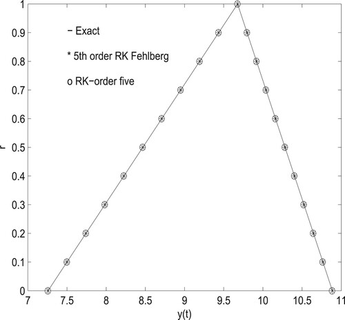
Table 1. Approximate Solution by RK-5 and RKF-5.

	R-K order five		RKF-5
r	$\underset{\_}{y}(t_i;r)$	$\overline{y}(t_i;r)$	$\underset{\_}{y}(t_i;r)$	$\overline{y}(t_i;r)$
0	7.2577293788874	10.886594068331	7.2577315354883	10.886597303232
0.1	7.4996536915170	10.765631912016	7.4996559200046	10.765635110974
0.2	7.7415780041465	10.644669755701	7.7415803045209	10.644672918716
0.3	7.9835023167761	10.523707599386	7.9835046890372	10.523710726458
0.4	8.2254266294057	10.402745443072	8.2254290735535	10.402748534200
0.5	8.4673509420353	10.281783286757	8.4673534580697	10.281786341941
0.6	8.7092752546649	10.160821130442	8.7092778425860	10.160824149683
0.7	8.9511995672944	10.039858974127	8.9512022271023	10.039861957425
0.8	9.1931238799240	9.9188968178128	9.1931266116186	9.9188997651674
0.9	9.4350481925536	9.7979346614980	9.4350509961349	9.7979375729093
1.0	9.6769725051832	9.6769725051832	9.6769753806511	9.6769753806511

Table 2. Exact solution.

	Exact solution
r	$\underset{\_}{y}(t_i;r)$	$\overline{y}(t_i;r)$
0	7.2577317542683	10.886597631402
0.1	7.4996561460772	10.765635435498
0.2	7.7415805378862	10.644673239593
0.3	7.9835049296951	10.523711043689
0.4	8.2254293215041	10.402748847784
0.5	8.4673537133130	10.281786651880
0.6	8.7092781051220	10.160824455975
0.7	8.9512024969309	10.039862260071
0.8	9.1931268887398	9.9189000641667
0.9	9.4350512805488	9.7979378682622
1.0	9.6769756723577	9.6769756723577

Table 3. Error in R-K order five and fifth-order R-K Fehlberg method.

	Error in R-K order five		Error in R-K Fehlberg method
r	$\underset{\_}{Y}(t_i;r)$	$\overline{Y}(t_i;r)$	$\underset{\_}{Y}(t_i;r)$	$\overline{Y}(t_i;r)$
0	2.3753809$\times {10}^{-6}$	3.5630714$\times {10}^{-6}$	2.187799$\times {10}^{-7}$	3.281699$\times {10}^{-7}$
0.1	2.4545602$\times {10}^{-6}$	3.5234817$\times {10}^{-6}$	2.260726$\times {10}^{-7}$	3.245236$\times {10}^{-7}$
0.2	2.5337396$\times {10}^{-6}$	3.4838921$\times {10}^{-6}$	2.333652$\times {10}^{-7}$	3.208773$\times {10}^{-7}$
0.3	2.6129190$\times {10}^{-6}$	3.4443023$\times {10}^{-6}$	2.406579$\times {10}^{-7}$	3.172309$\times {10}^{-7}$
0.4	2.6920983$\times {10}^{-6}$	3.4047126$\times {10}^{-6}$	2.479506$\times {10}^{-7}$	3.135846$\times {10}^{-7}$
0.5	2.7712777$\times {10}^{-6}$	3.3651229$\times {10}^{-6}$	2.552432$\times {10}^{-7}$	3.099382$\times {10}^{-7}$
0.6	2.8504571$\times {10}^{-6}$	3.3255333$\times {10}^{-6}$	2.625359$\times {10}^{-7}$	3.062920$\times {10}^{-7}$
0.7	2.9296364$\times {10}^{-6}$	3.2859436$\times {10}^{-6}$	2.698286$\times {10}^{-7}$	3.026456$\times {10}^{-7}$
0.8	3.0088158$\times {10}^{-6}$	3.2463539$\times {10}^{-6}$	2.771212$\times {10}^{-7}$	2.989992$\times {10}^{-7}$
0.9	3.0879952$\times {10}^{-6}$	3.2067642$\times {10}^{-6}$	2.844139$\times {10}^{-7}$	2.953529$\times {10}^{-7}$
1.0	3.1671745$\times {10}^{-6}$	3.1671745$\times {10}^{-6}$	2.917066$\times {10}^{-7}$	2.917066$\times {10}^{-7}$

4.2. Example

Consider the HFIVP [25, 26], (7) $\{\begin{array}{ll}{y}^{\mathrm{\prime }}(t)=y(t)+j(t){\xi }_{k}y(t_k),& t\in [t_k,t_{k+1}],t_k=k,k=0,1,2,3,\dots ,\\ y(t;r)=[(0.75+0.25r){\mathrm{e}}^t,(1.125-0.125r){\mathrm{e}}^t],& 0\le r\le 1,\end{array}$(7) where, $\begin{array}{rl}j(t)& =|\sin (\mathrm{\pi t})|,k=0,1,2,\dots ,\\ {\xi }_k(\mu )& =\{\begin{array}{ll}\hat{0},& \text{if}k=0\\ \mu ,& \text{if}k\in \{1,2,\dots \}.\end{array}\end{array}$Then $y(t)+j(t){\xi }_k(y(t_k)$ is continuous function of t, y and ${\xi }_k(y(t_k).$ solving similar to the previous example we obtain the numerical results as follows $\begin{array}{rl}y(1;r)& =[(0.75+0.25r)e,(1.125-0.125r)e],\\ y(2;r)& =(\frac{\pi }{{\pi }^2+1}+e(1+\frac{\pi }{{\pi }^2+1}))y(1;r).\end{array}$Then $y(2.0;1)$ is approximately 10.31033432 where as $y_1(2.0;1)$ is approximately 10.31033708. The exact and approximate solutions by RKF-5 and RK-5 are compared and plotted at t = 2(see Tables 4, 5 and Figure 2), and error in RKF-5 and RK-5 is given at t = 2 (See Table 6).

Figure 2. Comparison of exact and approximate solutions (for h$=0.1$, t$=2$).

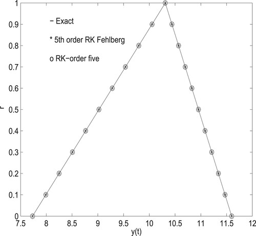
Table 4. Approximate Solution by RK-5 and RKF-5.

	R-K order five		RKF-5
r	$\underset{\_}{y}(t_i;r)$	$\overline{y}(t_i;r)$	$\underset{\_}{y}(t_i;r)$	$\overline{y}(t_i;r)$
0	7.7327611483619	11.599141722542	7.7327508000140	11.599126200021
0.1	7.9905198533073	11.470262370070	7.9905091600145	11.470247020020
0.2	8.2482785582527	11.341383017597	8.2482675200150	11.341367840020
0.3	8.5060372631981	11.212503665124	8.5060258800154	11.212488660020
0.4	8.7637959681435	11.083624312652	8.7637842400159	11.083609480020
0.5	9.0215546730889	10.954744960179	9.0215426000164	10.954730300019
0.6	9.2793133780343	10.825865607706	9.2793009600169	10.825851120019
0.7	9.5370720829797	10.696986255234	9.5370593200173	10.696971940019
0.8	9.7948307879251	10.568106902761	9.7948176800178	10.568092760019
0.9	10.052589492870	10.439227550288	10.052576040018	10.439213580019
1.0	10.310348197815	10.310348197815	10.310334400018	10.310334400018

Table 5. Exact solution.

	Exact Solution
r	$\underset{\_}{y}(t_i;r)$	$\overline{y}(t_i;r)$
0	7.7327507380331	11.599126107049
0.1	7.9905090959676	11.470246928082
0.2	8.2482674539020	11.341367749115
0.3	8.5060258118364	11.212488570148
0.4	8.7637841697709	11.083609391180
0.5	9.0215425277053	10.954730212213
0.6	9.2793008856398	10.825851033246
0.7	9.5370592435742	10.696971854279
0.8	9.7948176015086	10.568092675312
0.9	10.052575959443	10.439213496344
1.0	10.310334317377	10.310334317377

Table 6. Error in R-K order five and fifth-order R-K Fehlberg method.

	Error in R-K order five		Error in RKF-5
r	$\underset{\_}{Y}(t_i;r)$	$\overline{Y}(t_i;r)$	$\underset{\_}{Y}(t_i;r)$	$\overline{Y}(t_i;r)$
0	1.0410328$\times {10}^{-5}$	1.5615493$\times {10}^{-5}$	6.19809$\times {10}^{-8}$	9.29714$\times {10}^{-8}$
0.1	1.0757339$\times {10}^{-5}$	1.5441987$\times {10}^{-5}$	6.40469$\times {10}^{-8}$	9.19384$\times {10}^{-8}$
0.2	1.1104350$\times {10}^{-5}$	1.5268482$\times {10}^{-5}$	6.61129$\times {10}^{-8}$	9.09054$\times {10}^{-8}$
0.3	1.1451361$\times {10}^{-5}$	1.5094976$\times {10}^{-5}$	6.81790$\times {10}^{-8}$	8.98723$\times {10}^{-8}$
0.4	1.1798372$\times {10}^{-5}$	1.4921471$\times {10}^{-5}$	7.02450$\times {10}^{-8}$	8.88393$\times {10}^{-8}$
0.5	1.2145383$\times {10}^{-5}$	1.4747965$\times {10}^{-5}$	7.23110$\times {10}^{-8}$	8.78062$\times {10}^{-8}$
0.6	1.2492394$\times {10}^{-5}$	1.4574460$\times {10}^{-5}$	7.43771$\times {10}^{-8}$	8.67733$\times {10}^{-8}$
0.7	1.2839405$\times {10}^{-5}$	1.4400954$\times {10}^{-5}$	7.64431$\times {10}^{-8}$	8.57403$\times {10}^{-8}$
0.8	1.3186416$\times {10}^{-5}$	1.4227449$\times {10}^{-5}$	7.85091$\times {10}^{-8}$	8.47072$\times {10}^{-8}$
0.9	1.3533427$\times {10}^{-5}$	1.4053943$\times {10}^{-5}$	8.05752$\times {10}^{-8}$	8.36742$\times {10}^{-8}$
1.0	1.3880438$\times {10}^{-5}$	1.3880438$\times {10}^{-5}$	8.26412$\times {10}^{-8}$	8.26412$\times {10}^{-8}$

5. Conclusion and discussion

The study emphasizes how important mathematical models are, especially when dealing with complex systems that have both discrete and continuous behaviors. Fuzzy hybrid differential equations present a flexible analytical tool that is effective in capturing the fuzziness that is inherent in real-world phenomena. Of the various approaches that can be used, the rarely studied Runge-Kutta Fehlberg scheme stands out as an excellent option to address the complex problems that hybrid fuzzy systems present. The introduction of the fifth-order Runge-Kutta Fehlberg algorithm is crucial, demonstrating how well it can handle the intricacy of hybrid fuzzy differential equations and produce accurate and consistent solutions in the end.

Moreover, this work's contribution goes beyond simple theoretical investigation. This work establishes the foundation for real-world applications in a variety of domains by presenting the idea of hybrid differential equations and then converting them into fuzzy hybrid differential equations. A major breakthrough in computational techniques, the Runge-Kutta Fehlberg method of order 5 for solving FHDEs promises improved accuracy and dependability.

A comparison of the traditional fifth-order Runge-Kutta method and the Runge-Kutta Fehlberg method provides strong evidence for the superiority of the former. It is clear from careful inspection and error analysis that the RKF-5 approach performs better than the other one, providing answers that are closer to the exact answers. While there are differences between RKF-5 and RK-5 solutions, the fact that they agree with exact solutions highlights how reliable and effective both approaches are.

All things considered, this work not only advances our knowledge of mathematical modeling in complex systems but also emphasizes the usefulness and consistency of the Runge-Kutta Fehlberg approach. It opens the door to more precise and effective computational methods for solving fuzzy hybrid differential equations, enhancing mathematical modeling and analysis across a variety of domains. This is achieved by connecting theoretical understanding with empirical validation.

Author contributions:

All the authors contributed equally to the preparation of the complete manuscript.

Disclosure statement

No potential conflict of interest was reported by the author(s).

Additional information

Funding

This research was not supported by any type of funds.

References

- Rangasamy M, hesneau C, Martin-Barreiro C, et al. On a novel dynamics of SEIR epidemic models with a potential application to COVID-19. Symmetry. 2022;14:1–19.
- Rangasamy M, Alessa N, Dhandapani PB, et al. Dynamics of a novel IVRD pandemic model of a large population over a long time with efficient numerical methods. Symmetry. 2022;1919:1–17.
- Kalpana U, Balaganesan P, Renuka J, et al. On the decomposition and analysis of novel simultaneous SEIQR epidemic model. AIMS Math. 2023;10:5918–5933.
- Zeb A, Alzahrani E, Erturk VS, et al. Mathematical model for coronavirus disease 2019 (COVID-19) containing isolation class. Biomed Res Int. 2020;2020:7. Article ID 3452402. doi:10.1155/2020/3452402
- Zeb A, Zaman G, Momani S. Square-root dynamics of a giving up smoking model. Appl Math Model. 2013;37(7):5326–5334. doi: 10.1016/j.apm.2012.10.005
- Bushnaq S, Saeed T, Torres DFM, et al. Control of COVID-19 dynamics through a fractional-order model. Alex Eng J. 2021;60(4):3587–3592. doi: 10.1016/j.aej.2021.02.022
- Zeb A, Atangana A, Khan ZA, et al. A robust study of a piecewise fractional order COVID-19 mathematical model. Alex Eng J. 2022;61(7):5649–5665. doi: 10.1016/j.aej.2021.11.039
- Nazir G, Zeb A, Shah K, et al. Study of COVID-19 mathematical model of fractional order via modified Euler method. Alex Eng J. 2021;60(6):5287–5296. doi: 10.1016/j.aej.2021.04.032
- Zadeh LA. Fuzzy sets. Inf Control. 1965;8:338–353. doi: 10.1016/S0019-9958(65)90241-X
- Kaleva O. Fuzzy differential equations. Fuzzy Sets Syst. 1987;24:301–317. doi: 10.1016/0165-0114(87)90029-7
- Kaleva O. The Cauchy problem for fuzzy differential equations. Fuzzy Sets Syst. 1990;35:389–396. doi: 10.1016/0165-0114(90)90010-4
- Kloeden PE. Fuzzy dynamical systems. Fuzzy Sets Syst. 1982;7:275–296. doi: 10.1016/0165-0114(82)90056-2
- Lakshmikantham V. Uncertain systems and fuzzy differential equations. J Math Anal Appl. 2000;251:805–817. doi: 10.1006/jmaa.2000.7053
- Veeresha P, Prakasha DG, Kumar S. A fractional model for propagation of classical optical solitons by using nonsingular derivative. Math Meth Appl Sci. 2020;2020:1–15. doi: 10.1002/mma.6335
- Khan MA, Ullah S, Kumar S. A robust study on 2019-nCOV outbreaks through non-singular derivative. Eur Phys J Plus. 2021;168:136. doi: 10.1140/epjp/s13360-021-01159-8
- Ghanbari B, Kumar S. A study on fractional predator–prey–pathogen model with Mittag–Leffler kernel-based operators. Numer Methods Partial Differ Equ. 2024;40:e22689. doi: 10.1002/num.22689
- Kumar S, Kumar A, Samet B, et al. A study on fractional host–parasitoid population dynamical model to describe insect species. Numer Methods Partial Differ Equ. 2021;37:1673–1692. doi: 10.1002/num.22603
- Kumar S, Kumar R, Momani S, et al. A study on fractional COVID-19 disease model by using Hermite wavelets. Math Meth Appl Sci. 2023;46(7):7671–7687. doi: 10.1002/mma.7065
- Kumar S, Chauhan RP, Momani S, et al. Numerical investigations on COVID-19 model through singular and non-singular fractional operators. Numer Methods Partial Differ Equ. 2024;40(1):e22707. doi: 10.1002/num.22707
- Lakshmikantham V, Liu XZ. Impulsive hybrid systems and stability theory. Int J Nonlinear Differ Equ. 1999;5:9–17.
- Lakshmikantham V, Mohapatra RN. Theory of fuzzy differential equations and inclusions. United Kingdom: Taylor and Francis; 2003.
- Sambandham M. Perturbed Lyapunov-like functions and hybrid fuzzy differential equations. Int J Hybrid Syst. 2002;2:23–34.
- Pederson S, Sambandham M. The Runge-Kutta method for hybrid fuzzy differential equations. Nonlinear Anal Hybrid Syst. 2008;2:626–634. doi: 10.1016/j.nahs.2006.10.013
- Johansson KH, Lygeros J, Sastry S. Control systems, robotics and automation – Vol. XV – modeling of hybrid systems, 2004.
- Jayakumar T, Kanagarajan K. Numerical solution for hybrid fuzzy system by Runge-Kutta method of order five. Int J Appl Math Sci. 2012;6:3591–3606.
- Jayakumar T, Kanagarajan K. Numerical solution for hybrid fuzzy system by Runge-Kutta Fehlberg method. Int J Math Anal. 2012;6:2619–2632.
- Dhandapani PB, Thippan J, Bundit U, et al. On new solutions of fuzzy hybrid differential equations by novel approaches. J Math. 2023;2023:1–18. doi: 10.1155/2023/7865973Article Id 7865973.