Deep learning with convolutional neural networks for EEG-based music emotion decoding and visualization

Abstract

Purpose: Emotion is the reflection of individual's perception and understanding of various things, which needs the synergy of various brain regions. A large number of emotion decoding methods based on electroencephalogram (EEG) have been proposed. But extracting the most discriminative and cognitive features to construct a model is yet to be determined. This paper aims to construct a model that can extract the most discriminative and cognitive features.

Materials and methods: Here, we collected EEG signals from 24 subjects in a musical emotion induction experiment. Then, an end-to-end branch LSTM-CNN (BLCNN) was used to extract emotion features from the laboratory dataset and DEAP dataset for emotion decoding. Finally, the extracted features were visualized on the laboratory dataset using saliency map.

Result: The classification results showed that the accuracy of the three classification of the laboratory dataset was 95.78% ± 1.70%, and the accuracy of the four classification of the DEAP dataset was 80.97% ± 7.99%. We found that the discriminating features of positive emotion were distributed in the left hemisphere, at the same time, negative emotion features were distributed in the right hemisphere, where mainly in the frontal, parietal and occipital lobes.

Conclusion: In this paper, we proposed a neural network model, namely BLCNN. The model obtained good results in laboratory dataset and DEAP dataset. Through the visual analysis of the features extracted by BLCNN, it was found that the features were consistent with emotional cognition. Therefore, this paper provided a new perspective for the practical application of human-computer emotional interaction.

Keywords:

• EEG
• emotion
• CNN
• LSTM
• deep learning
• visualization

1. Introduction

Emotion reflects people’s perception and cognition of various things. It contains a variety of components, including subjective experience, cognitive process, behavioral expression, psychological and physiological changes [1]. Emotions play an important role in daily life. For example, if a person cannot deal with emotional fluctuations properly caused by psychological or physical injury, psychological disorders such as autism and depression may be developed [2]. Over the past few decades, there has been a growing body of research on emotions in a wide range of fields, including psychology [3], medicine [4], social [5] and computer science [6].

In the experiment of studying emotions, it is the premise of effective research to select the appropriate inducing method and produce emotion successfully. Researchers often use auditory, visual or audio-visual stimuli with emotional content to induce different emotions in subjects. For example, Tian et al. [7] designed an emotion induction experiment by using faces with emotion and no external features as stimulus materials, and different faces were used to induce different emotional states of the subjects. Koelstra et al. [8] used music video clips with emotions as stimulus materials to design an experiment, which recorded participants' emotional state scores, physiological signals, facial expressions and electroencephalogram (EEG) data, and established a multi-modal dataset for analyzing human emotional states. Zheng et al. [9] used movies with emotions as stimulus materials to conduct an emotion induction experiment. Different movie clips were used to induce different emotional states of the subjects. In Zheng’s experiment, happiness, sadness, fear or neutral emotional states of the subjects and EEG data and eye movement information were collected. In auditory stimulation, music is art with great emotional rendering power, which has a great guiding effect on the audience's emotions [10]. Music can elicit deeper and longer emotional experiences than any other stimulus material. Therefore, this paper adopts the EEG data of music-induced emotion collected by our laboratory to conduct emotion recognition research.

In recent years, many emotion recognition methods based on EEG have been proposed. Liu et al. [11] proposed a new deep neural network for emotion classification, which combined convolutional neural network (CNN), sparse auto encoder (SAE) and deep neural network (DNN) for recognition research. Liu’s method was applied to the DEAP dataset, and the highest recognition accuracy of valence and arousal was 89.49% and 92.86%, respectively. In the SEED dataset, the best recognition accuracy reached 96.77%. Salama et al. [12] used a multi-channel EEG signal to construct a 3 D data representation and used it as data input of the 3 D CNN model. DEAP dataset was used to validate the method, and the recognition accuracy of valence and arousal reached 87.44% and 88.49%, respectively. Although these methods all use neural networks for feature extraction and classification, the EEG data need to be transformed before entering neural networks, which increases the computational complexity in the real-time application and is not conducive to the construction of BCI. Moreover, the process of deep learning is like a black box: its internal mechanism is unknown [13]. Therefore, we should not only pay attention to the accuracy of classification but also pay attention to whether the features extracted by CNN conform to the relevant cognitive characteristics.

To solve the above problems, this paper proposed an end-to-end deep learning model, BLCNN, which did not require complex EEG data conversion processes. BLCNN used a dual-branch structure to extract features from EEG signals. One branch used CNN to extract temporal and spatial features, while the other branch used long short term memory (LSTM) to extract time series features. The features extracted from the two branches were concatenated, and then emotion recognition was performed. Finally, a saliency map was used to visualize the features and explored whether the features extracted by our model conform to the cognitive characteristics.

2. Materials and methods

2.1. Participants

Twenty-four healthy students (14 males, average age: 18.50 ± 0.91 years old) from Chongqing University of Posts and Telecommunications participated in the experiment. None of them had mental or neurological problems. Each subject had normal or corrected visual acuity and was right-handed. The subjects received appropriate monetary compensation after the experiment.

2.2. EEG experiment

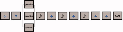
Participants were asked to listen to 18 pieces of music and rate each piece of music for valence, arousal, familiarity, and liking using the self-assessment mannequin (SAM). The music was divided into three types, corresponding to different emotions (positive, neutral and negative). Each type of emotion had 6 pieces of music, divided into 6 blocks, and each block contained three pieces of music that contained positive, neutral and negative emotions. Each piece of music was then composed of three 20 seconds clips. Each block was composed of the following parts: (1) Spontaneous EEG acquisition in the first 10 seconds; (2) Music attribute prompt for 3 seconds;(3) 20 seconds of music clips and 3 seconds of spontaneous EEG recordings were repeated 3 times;(4) Spontaneous EEG acquisition for 10 seconds; (5) Complete SAM. There are 9 trials in the whole block, including 3 trials of positive emotion, 3 trials of neutral emotion, and 3 trials of negative emotion. Each block of the experiment is shown in Figure 1.

Figure 1. Design of each block of the experiment.

2.3. EEG recording

Subjects were asked to sit in a comfortable chair and listen to a music clip through headphones while focusing on the cross symbol on the screen. During the experiment, subjects were asked to remain relaxed and awake. A 64-channel Neuracle acquisition device was used to acquire EEG data. The sampling rate was set to 1000 Hz, meanwhile, the recording reference was set to the vertex, and all electrode impedance was kept at 5 kΩ online.

2.4. Data processing

The collected data were down-sampled from the original sampling rate of 1000 Hz to 250 Hz, and band-pass filtered from 0.1 to 80 Hz. In order to eliminate the interference from the electric supply, the data had been filtered with a 50 Hz notch. Finally, perform operations such as artefact removal, re-reference and baseline correction on the EEG data.

A total of 55 electrodes (Fp1/2, AF3/4, AF7/8, Fz, F1/2, F3/4, F5/6, F7/8, FCz, FC1/2, FC3/4, FC5/6, FT7/8, Cz, C1/2, C3/4, C5/6, T7/8, CP1/2, CP3/4, CP5/6, TP7/8, Pz, P3/4, P5/6, P7/8, POz, PO3/4, PO7/8, O1/2) were used for our analysis. After pre-processing, each trial of length 20 s is divided into 20 epochs of length 1 s used as input to the neural network.

2.5. DEAP dataset

DEAP (http://www.eecs.qmul.ac.uk/mmv/datasets/deap/) is a multimodal dataset used to analyse human emotional states [8]. During the experiment, 32 participants watched 40 one-minute music videos while EEG and peripheral physiological signals were recorded. At the end of each trial, participants self-rated their arousal (calm to excited), valence (unhappy to happy), and liking (dislike to like) indicators. Here, a 10–20 system was used to collect 32 channels of EEG signals with a sampling frequency of 512 Hz. The other eight channels record peripheral physiological signals such as skin temperature, blood volume, electromyography and galvanic skin response. In this paper, only EEG data were used for analysis. Each EEG data was downsampled to 128 Hz, then the artefacts were removed, and finally, band-pass filtering and average re-reference were performed at 4–45Hz.

In terms of data division of DEAP dataset, we deleted baseline data, 3 seconds after the beginning and 3 seconds before the end of each trial, and then divided the remaining 54 seconds of data into 18 epochs, each with a length of 3 seconds. We used the valence-arousal (VA) model and divided the valence arousal space into four parts: low arousal-low valence (LALV), high arousal-low valence (HALV), low arousal-high valence (LAHV) and high arousal-high valence (HAHV). Similar to the literature [14], we also added a gap in the VA space to retain data with wake and potency scores between 4.8 and 5.2.

2.6. Proposed model

The framework of our model (BLCNN) was shown in Figure 2, which consisted of two modules: time sequence feature extractor and time and space feature extractor. The input to both modules is the EEG signals after pre-processing. The sequential feature extractor used two layers of LSTM to capture temporal features recorded by multi-channel EEG. The time and space feature extractor used CNN to obtain the spatial and temporal features of EEG signals respectively.

Figure 2. BLCNN model structure.

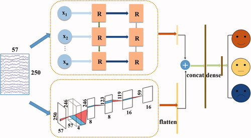
In the sequential feature extractor, two layers of LSTM were used. The number of hidden neurons was 64. In the output sequence, a single hidden state value was returned. In the time and space feature extractor, CNN was used. The first layer was composed of four convolution kernels with a size of 1 × 5, and each kernel performed the convolution of time. The second layer was composed of eight convolution kernels with a size of a number of channels × 1. Each convolution kernel performed spatial filtering on all possible electrode pairs and weighted the previous temporal convolution filters. The third layer used a maximum pooling layer with a size of 1 × 2 to reduce the dimension of data. In the fourth layer, 16 convolution kernels with a size of 1 × 5 were used to further extract time features. In the fifth layer, a maximum pooling layer with a size of 1 × 2 was used to further reduce the dimension of features. Finally, the extracted features were flattened. In order to prevent the gradient disappearance and explosion, we add batch normalization [15] and linear activation function ReLU [16] after the second and fourth layers. To solve the problem of overfitting the model during training, dropout technology was used [17]. Finally, the features extracted by the two branches were concatenated by columns and input into a dense layer.

2.7. Model Training

We used the ten-fold cross-validation strategy to train the data of each subject separately. Next, we used the softmax function to calculate the final probability distribution and used the cross entropy loss function to optimize. To prevent model overfitting, we set the dropout value to 0.5. Adam optimizer with a 0.001 learning rate was used in the model, and the Batch size value was set to 32.

2.8. Saliency map

For feature visualization of a neural network, we used a Saliency map, the essence of a Saliency map is the gradient of CNN output relative to its input. A saliency map is often applied to images, such as one image $I,$ corresponding to the category t. Our model $S_t(I)$ is a linear model, as shown below: (1) $$S_t\left(I\right)=W_t^{T}I+b_t$$(1)

where $w_t$ and $b_t$ are the weights and biases of the classification model, and $I$ is the input image. Then we can see the corresponding important information of each pixel by observing the size of $w_t.$ EEG signals can be viewed as images when using a saliency map.

For deep neural networks, model $S_t\left(I\right)$ is a complex nonlinear function, and the above inferences about linear functions are not suitable, so another inference is required at this time. For a given image $I,$ a first-order Taylor expansion of the model $S_t(I)$ can be performed around $I$ as follows: (2) $$S_t\left(I\right)\approx W_t^{T}I+b_t$$(2)

where $w$ is the derivative of the model $S_t(I)$ with respect to $I$ at point $I_0.$ (3) $$w={\displaystyle {\frac{\partial S_t}{\partial I}|}_{I_0}}$$(3)

Therefore, we need to calculate the value of $w,$ and then we can calculate the important information corresponding to each pixel, and finally get the gradient of the CNN output relative to the input.

3. Results

3.1. Classification results and evaluation

The music emotion data collected by our laboratory were applied to the proposed model. It was compared with the traditional machine learning classification method Support Vector Machine (SVM) [18] and two classical reproductions of deep learning models (DeepNet and ShallowNet) [19]. The classification and evaluation results of each classifier applied to the laboratory dataset were shown in Table 1 and Figure 3, and the classification and evaluation results of the DEAP dataset were shown in Table 2 and Figure 4. In three classifications (positive, neutral and negative) accuracy of our BLCNN in the laboratory dataset reached 95.78% ± 1.70%. The accuracy of the four classifications (HAHV vs. HALV vs. LAHV vs. LALV) in the DEAP dataset reached 80.97% ± 7.99%. As be seen from the performance of each classifier, our BLCNN had superior performance both in classification accuracy and in the number of model parameters. We used the confusion matrix to evaluate the performance of our BLCNN in emotion recognition. In Figure 5, neutral and negative emotions were better identified in the laboratory dataset, and HAHV was better identified in the DEAP dataset. In general, this model was robust and effective in emotion recognition.

Figure 3. Average classification results of laboratory dataset on different classifiers.

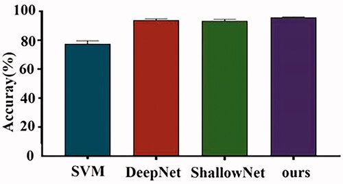
Figure 4. Average classification results of DEAP dataset on different classifiers.

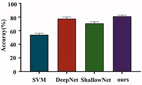
Figure 5. Classification confusion matrix for two kinds of datasets. (a) Confusion matrix for laboratory dataset. (b) Confusion matrix for DEAP dataset.

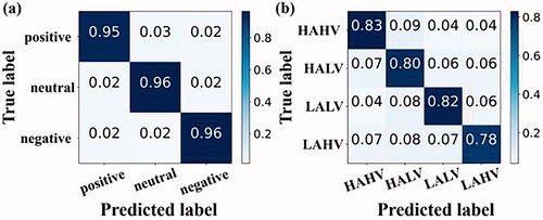
Table 1. Training results and evaluation in laboratory dataset (%).

Method	Accuracy	Macro precision	Macro recall	Params
SVM	77.48 ± 10.27	78.24 ± 10.16	77.48 ± 10.49	$-$
DeepNet	93.89 ± 4.39	94.62 ± 3.25	93.89 ± 4.49	175503
ShallowNet	93.38 ± 5.36	93.57 ± 5.37	93.38 ± 5.47	95523
Ours	95.78 ± 1.70	95.85 ± 1.71	95.78 ± 1.74	69891

Table 2. Training results and evaluation in DEAP dataset (%).

Method	Accuracy	Macro precision	Macro recall	Params
SVM	53.84 ± 10.08	54.04 ± 11.09	53.84 ± 11.06	$-$
DeepNet	77.57 ± 11.43	82.06 ± 9.05	77.61 ± 11.72	174,279
ShallowNet	70.56 ± 11.02	72.93 ± 10.49	70.47 ± 11.35	72,564
Ours	80.97 ± 7.99	81.52 ± 8.20	80.97 ± 8.19	68180

3.2. Feature visualization

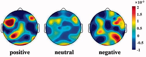
A saliency map was used for feature visualization. The closer the gradient value was to the two ends, the more discriminative the feature was in classification. The saliency map was calculated in the laboratory dataset, and then the gradients of different emotions of all subjects were averaged. Finally, the results were plotted on the topographic map of the head (as shown in Figure 6). It can be seen from Figure 6 that the features with discrimination for emotion classification were distributed in the frontal lobe, parietal lobe, occipital lobe. For positive emotions, the features with discrimination were mainly distributed in the left brain region, while for negative emotions, the features with discrimination were mainly distributed in the right brain region, namely emotions have hemispheric asymmetry.

Figure 6. Visualization of features extracted from laboratory dataset by BLCNN.

4. Discussion

In order to demonstrate the effectiveness of our model, our proposed model was validated in the laboratory emotion dataset and DEAP dataset. Tables 1 and 2, and Figures 3 and 4 showed the comparison of classification performance between our method and classical models. It can be seen that the model we proposed had the least number of parameters among these models, and in terms of accuracy, the accuracy of our model reached 95.78% ± 1.70% in the laboratory dataset, the accuracy of the DEAP dataset is 80.97% ± 7.99%. In terms of the number of parameters and classification accuracy, our model demonstrated superior performance in emotion recognition.

Deep learning has shown its superior classification performance in various fields, but the interpretability of the deep learning model has always been a concern of people. Therefore, a Saliency map was used to visualize the features extracted by our model to explore whether the features proposed by the model are consistent with the cognitive characteristics of emotions. As can be seen from Figure 6, the most discriminating features extracted from positive emotions were mainly distributed in the left frontal lobe, left parietal lobe and occipital lobe. Negative emotions were mainly distributed in the right frontal lobe, right parietal lobe and occipital lobe. Generally speaking, positive emotions were distributed in the left brain regions, while negative emotions were distributed in the right brain regions, presenting hemispheric asymmetry. Just as Schmidt et al. [20] found that asymmetric frontal EEG activity patterns differentiated the valence of music excerpts, subjects showed greater relative left frontal EEG activity under happy music clips and greater right frontal EEG activity under fearful and sad music clips. Similarly, Ahern et al. [21] observed different lateralization of positive and negative emotions in the frontal lobe, with activation of the relative left hemisphere of positive emotion and activation of the relative right hemisphere of negative emotion. Wheeler et al. [22] found that larger activation of the left frontal lobe was associated with stronger positive movies, while larger activation of the right frontal lobe was associated with stronger negative movies. Lin et al. [23] found that features from the frontal and parietal lobes can provide identification information related to affective processing. Zhuang et al. [24] found that the prefrontal and occipital lobes were prominent in identifying emotions. It can be seen from these research results that the features extracted by our proposed model were consistent with the emotional cognition mechanism.

5. Conclusion

In this work, we proposed a BLCNN model, which had achieved good results in both the laboratory dataset and DEAP dataset. The visualization results showed that our proposed model conformed to the emotion cognitive characteristics in terms of feature extraction. Our work could provide a new perspective on human-computer emotional interaction in practical applications.

Disclosure statement

The authors declare that the research was conducted in the absence of any commercial or financial relationships that could be construed as a potential conflict of interest.

Additional information

Funding

The present research was supported by the Nature Science Foundation of Chongqing (cstc2019jcyj-msxmX0275) and the Chongqing Graduate Research and Innovation Projects (#CYS21325).

References

- Bradley MM, Lang PJ. Emotion and motivation. In: Handbook of Psychophysiology. New York: Cambridge University Press; 2007. p. 581–607.
- Gross JJ, Muñoz RF. Emotion regulation and mental health. Clin Psychol Sci Pract. 1995;2(2):151–164.
- C. G L. The mechanism of the emotions. Classical Psychol. 1885;:672–684.
- Ofri D. What doctors feel: how emotions affect the practice of medicine. Boston, MA: Beacon Press; 2013.
- Burkitt I. Social relationships and emotions. Sociology. 1997;31(1):37–55.
- Liu Y, Fu Q, Fu X. The interaction between cognition and emotion. Chin Sci Bull. 2009;54(22):4102–4116.
- Tian Y, Zhang H, Pang Y, et al. Classification for single-trial N170 during responding to facial picture with emotion. Front Comput Neurosci. 2018;12:68.
- Koelstra S, Muhl C, Soleymani M, et al. Deap: a database for emotion analysis; using physiological signals. IEEE Trans Affective Comput. 2011;3(1):18–31.
- Zheng W-L, Liu W, Lu Y, et al. Emotionmeter: a multimodal framework for recognizing human emotions. IEEE Trans Cybern. 2019;49(3):1110–1122.
- Krumhansl CL. An exploratory study of musical emotions and psychophysiology. Can J Exp Psychol. 1997;51(4):336–353.
- Liu J, Wu G, Luo Y, et al. EEG-based emotion classification using a deep neural network and sparse autoencoder. Front Syst Neurosci. 2020;14:43.
- Salama ES, A. El-Khoribi R, E. Shoman M, et al. EEG-based emotion recognition using 3D convolutional neural networks. IJACSA. 2018;9(8):329–337.
- Yosinski J, Clune J, Nguyen A, et al. “Understanding neural networks through deep visualization,” arXiv preprintarXiv:1506.065792015.
- Zheng W-L, Zhu J-Y, Lu B-L. Identifying stable patterns over time for emotion recognition from EEG. IEEE Trans. Affective Comput. 2019;10(3):417–429.
- Ioffe S, Szegedy C. “Batch normalization: Accelerating deep network training by reducing internal covariate shift,” International conference on machine learning. PMLR, p. 448–456. 2015.
- Glorot X, Bordes A, Bengio Y. “Deep sparse rectifier neural networks,”Proceedings of the fourteenth international conference on artificial intelligence and statistics. JMLR Workshop and Conference Proceedings, p. 315–323. 2011.
- Srivastava N, Hinton G, Krizhevsky A, et al. Dropout: a simple way to prevent neural networks from overfitting. J Mach Learn Res. 2014;15(1):1929–1958.
- Duan R-N, Zhu J-Y, Lu B-L. Differential entropy feature for EEG-based emotion classification. In: 2013 6th International IEEE/EMBS Conference on Neural Engineering (NER). IEEE; 2013. p. 81–84.
- Schirrmeister RT, Springenberg JT, Fiederer LDJ, et al. Deep learning with convolutional neural networks for EEG decoding and visualization. Hum Brain Mapp. 2017;38(11):5391–5420.
- Schmidt LA, Trainor LJ. Frontal brain electrical activity (EEG) distinguishes valence and intensity of musical emotions. Cogn Emot. 2001;15(4):487–500.
- Ahern GL, Schwartz GE. Differential lateralization for positive and negative emotion in the human brain: EEG spectral analysis. Neuropsychologia. 1985;23(6):745–755.
- Wheeler RE, Davidson RJ, Tomarken AJ. Frontal brain asymmetry and emotional reactivity: a biological substrate of affective style. Psychophysiology. 1993;30(1):82–89.
- Lin Y-P, Wang C-H, Jung T-P, et al. EEG-based emotion recognition in music listening. IEEE Trans Biomed Eng. 2010;57(7):1798–1806.
- Zhuang N, Zeng Y, Yang K, et al. Investigating patterns for self-induced emotion recognition from EEG signals. Sensors. 2018;18(3):841.