Abstract
The Shewhart Xbar chart is effective in detecting large shifts in a process but unable to find moderate shifts. We show that this blind spot allows shifts smaller than one standard deviation to continue undetected for long periods, thereby incurring much larger total costs than do rapidly detected large shifts. Augmenting the Shewhart chart with a cumulative sum chart largely plugs this gap, leading to much more effective process monitoring.
Introduction
Quality control has always been open to improvement. Rather than being a tradition handed down from generation to generation, quality follows new techniques that do the job better. Do we not all have an enthusiasm and a new wave of interest for the Six Sigma™ quality procedures that have been presented? Were we not all impressed by the beautiful simplicity of the Shewhart control techniques when we first learned them? Shewhart's simple, sturdy charts have made their contribution for nearly a century, focusing users' attention on common and special causes. Recent Six Sigma thinking sharpens awareness of the value of more advanced statistical methods: As Citation5 asserts, “current business system + Six Sigma=TQM.”
This thinking has raised the technical statistical level from the computationally easy methods of the early twentieth century to such techniques (Citation7) as multifactorial designed experiments, response surfaces, robust design, and multiple regression. With these advances, there is also a need to improve on the basic Shewhart charts. The Xbar chart is effective in finding large changes in mean resulting from some special cause but cannot find small changes. This was previously felt tolerable since a small change incurs a small loss, so failing to detect it is not catastrophic. That reasoning is wrong and this article will help us to get a feeling of why this is so.
Statistical Formulation Of Step Change
When an industrial process is in control, it produces readings with mean (or central value) μ 0 and a standard deviation (or spread) σ 0. One reason for charting is to identify special causes in the process and make timely repair. Special causes can lead to a change in the mean or a change in the variability. We will concentrate on just changes in the mean, but our conclusions and warnings apply just as strongly to changes in the variability. So writing X i for the stream of process readings, we suppose that some special cause occurs at some time and changes the mean from the in-control value μ 0 to an out-of-control value μ 1. Examples of this sort of “persistent” special cause would be the point of a cutting tool chipping or a supplier sending a large batch of raw material that, unnoticed by anyone, was a little different than the current feedstock. The purpose of statistical process controls is to detect this change as soon as possible, diagnose the cause, and remove it or perhaps accommodate it by adjusting process settings.
The classic tool for this purpose is the Shewhart chart. The Shewhart I chart plots successive process readings along with a center line at μ
0 and control limits at 3 standard deviations from the central value μ
0. The Shewhart Xbar chart plots the means of “rational groups” of size m, say, and uses the same center line but has control limits at The control limits are wide enough that readings that fall outside them should be seriously investigated as evidence of special causes.
Another classical but less familiar chart is the cumulative sum (CUSUM) chart. See Citation2 for a brief description, and Citation3 for a deeper discussion. The DI (decision interval) CUSUM for an upward change in mean using “reference value” k somewhat above the in-control mean is defined by:
The CUSUM is attractive because it is the most powerful diagnostic there is for a step change from one value (the in-control mean) to another specified out-of-control value. To get this optimal test, you set the reference value k halfway between the in-control and the out-of-control mean.
We'll illustrate some aspects of CUSUM design with the problem of control of filling of bottles on a cola line. The following numbers, based on a textbook example (Citation6), are not real but intended to be realistic. Suppose the bottles have a nominal content of 12 oz of cola. The actual amount of cola in a bottle is not of course constant; let's suppose it follows a normal distribution with mean μ and standard deviation 0.25 oz. The mean μ is hard to set exactly, as it depends on environmental and other variables, but it is easy to adjust it upward or downward.
To avoid legal problems related to labeling, the manufacturer aims to set μ high enough that only 10% of bottles will have a content less than the nominal 12 oz. An easy calculation shows that this requires setting μ=12+1.28*0.25=12.32 oz, which is therefore the desired in-control mean.
If the mean μ drifts upward, you get bottles containing more cola than is required, which represents either a free gift to the consumer or wasted cola spilling from overfilled bottles. Suppose the cola costs the manufacturer $0.004 per oz and that the line fills 5000 bottles per hour. Then each 1-oz upward drift in μ costs $0.004*5000=$20 per hour, or $480 per day.
A daily loss of $120 would therefore correspond to a mean overfill of 0.25 oz, which is given by a mean of 12.32+0.25=12.57 oz. If you want to tune the CUSUM for maximum sensitivity to a shift of this magnitude, then you should use a reference value of (12.32+12.57)/2=12.445 oz.
The resulting CUSUM does not give the best possible performance if the mean actually changes to, say, 12.8 oz (for that change the optimal diagnostic would be a CUSUM using a reference value (12.32+12.80)/2=12.56 oz), but the performance of the CUSUM is quite robust in that it is close to optimal for the range of changes close to the change for which it was designed.
The “decision interval” is fixed by deciding how often you are willing to give a false alarm and diagnose a change that did not actually occur. The average run length (ARL) is the average number of observations seen up until when the chart signals.
The Shewhart chart, as commonly defined with 3-sigma control limits, has an ARL of 740 between false alarms of an upward change. When designing a CUSUM, you can choose the decision interval of the CUSUM to match this false alarm rate of the Shewhart or set it to give any other false-alarm rate you think advisable.
Calculating the decision interval that gives a particular in-control ARL is conveniently done using the software described in Citation3, which can be downloaded from the Web site www.stat.umn.edu/users/cusum/software.htm.
To illustrate use of the software, the following interchange with the program ANYGETH from the site shows how to find the appropriate decision interval so that the CUSUM has an in-control ARL of 740 readings, matching that of the Shewhart chart. The computer output is in regular type; the user responses in bold.
Which distribution do you want? (Give its number from this menu:)
1 Normal location
2 Normal variance
3 Poisson
4 Binomial
5 Negative binomial
6 Inv Gaussian mean
1
Give the in-control mean and standard deviation: 12.32 0.25
Give the out-of-control mean: 12.57
The reference value is 12.445
What are the Winsorizing constants?
(Say −999 999 if you don't want to winsorize or don't understand question:) −999 999
Want zero-start (say Z), steady state (say S) or FIR (say F?): Z
Enter ARL:
740
h 4.6810 arls 673.3 644.4 666.1
h 4.7739 arls 740.1 709.4 733.0
DI 1.193, IC ARL 740.1, OOC ARL 9.9, FIR ARL 6.1, SS ARL 5.9
Ignoring the winsorizing and start refinements to the basic CUSUM, the program tells you that the desired in-control ARL of 740 readings requires a decision interval of 1.193. It also reports that if the mean shifts to 12.57 right when you start the CUSUM, the ARL to detection will be 9.9 readings.
You can make the in-control ARL any value you like. For example, to cut down the false-alarm frequency from 1 in 740 to, say, 1 in 2000, you rerun ANYGETH and discover that this needs a decision interval of 1.439.
To complete the scheme, this CUSUM for an upward change is usually complemented by one for a downward change to achieve full control on the mean. The CUSUM for the downward change is defined by:
If you could live with a $120 per day overfill cost, but worried about a larger shift, perhaps $240 per day, resulting from a jump of 0.5 oz in the mean fill, then you would use a reference value of (12.32+12.82)/2=12.57. Getting an in-control ARL of 740 readings would need (as reported by ANYGETH) a decision interval of 0.629. If the mean were to go to 12.82 oz right after you started charting, the ARL to detection would be 3.3 readings.
These targets of $120 and $240 correspond (in this particular problem) to a mean shift by one standard deviation and two standard deviations, respectively. Expressing shifts in multiples of the standard deviation standardizes CUSUM problems; an in-control ARL of 740 for a CUSUM aimed at a one standard deviation shift requires a decision interval of 4.77 standard deviations, and an in-control ARL of 740 for a CUSUM tuned for a two standard deviation shift requires a decision interval of 2.52 standard deviations.
Following up a CUSUM Signal
A fringe benefit of controlling with a CUSUM is that it not only signals a shift but also estimates when the shift occurred and how large the shift is. Suppose that you use the CUSUM with k=12.445, h=1.193 oz, and that at reading number 273 the CUSUM has a value of 1.20, exceeding the decision interval. You follow the CUSUM back to where it most recently had the value 0. Suppose this was at reading 259. The estimated time when the shift occurred is then right after reading 259. The estimated magnitude of the shift is the slope of this last segment of the CUSUM, 1.20/(273−259)=0.086, plus the difference between the reference value and the in-control mean, 12.445−12.32=0.125. This gives the estimate 0.211 of the amount by which the current mean exceeds the in-control level. If you know the gain of the fill adjustment mechanism, this estimate then tells you how much adjustment is needed to bring the mean fill back to specification.
Detuning the CUSUM to Ignore Tiny Changes
As an aside, sometimes the CUSUM is too powerful to use in its native state. In the cola example, consider an upward shift in mean of 0.05 oz, to 12.37 oz, leading to a loss of $24 per day in overfill. It might be felt that $24 per day was not worth fixing or even knowing about, particularly if the mean fill had some random flutter, making small shifts like this a common occurrence. If this is the case, then you would like to design the CUSUM to have a long ARL at even this elevated level. This detuning is easily accomplished by doing the design plugging in the elevated mean for the in-control value. Running ANYGETH with an in-control mean of 12.37, and the same out-of-control target of 12.57, leads to k=12.47; setting the in-control ARL to 740 requires a decision interval of h=1.427.
You almost certainly would not want to detune the downward CUSUM; small downward shifts in mean lead to substantial increases in the percentage of underfilled bottles and legal troubles, so you would want the full power of the CUSUM for even small downward shifts.
The Importance Of Small But Not Tiny Changes
The Shewhart chart is well known not to be effective in detecting small to moderate changes in mean. This has apparently not bothered its users too much, as evidenced by the continuing widespread use of Shewhart charts without any backup chart (such as a CUSUM) for small changes. This can be rationalized by the argument that small changes incur small losses and so it does not matter if you can not detect them quickly.
For the cola filling example, suppose a bottle is sampled every 2 hours and its exact content measured. The cost of running at an elevated mean fill is directly proportional to the amount by which the mean fill exceeds the target level multiplied by the length of time for which the process runs at the elevated mean, i.e.;
We should mention another cost that we seem to overlook—the cost of stopping the process and trying to diagnose the special cause. This cost is a constant that is incurred whenever there is a signal—whether true or false. We will leave it out of the discussion because ignoring it does not affect the relative rankings of different charting methods so long as they are tuned for the same in-control run length.
Staying with our cola example and adding the performance of the SPC scheme, if the mean fill shifts to some level μ>12.32 oz and stays there until the SPC scheme gives a signal and the overfill is corrected, the expected loss will be:
Figure shows the expected loss for varying mean changes μ−μ 0 of three schemes—a Shewhart I chart; a CUSUM with k=0.5, h=4.77 standard deviations; and a CUSUM with k=1, h=2.52 standard deviations. (These are the two CUSUM designs developed above and aimed at losses of $120 and $240 per day, respectively.) The vertical axis is measured in dollars per incident and the horizontal axis in standard deviations. All three schemes are based on taking one reading every 2 hours and have an in-control ARL of 740 readings (and therefore 1480 hours) before a signal of an upward change. Table shows some of the numbers used to plot the figure.
Figure 1. Comparison of loss, cola example.
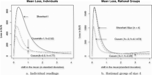
Table 1. Time to signal and loss
The shape of the curve for the Shewhart chart may be a surprise. There is a minimum around four standard deviations. Although the loss per unit time for a change this big is large, this loss is offset by the rapid detection of the change. Although not shown, larger changes in mean incur larger expected losses. This is no surprise since, even though the change is detected almost at once, some bad production slips through first. The surprise is how high the curve for the Shewhart chart goes for small changes. These changes are large enough to incur a perceptible penalty but small enough to escape quick detection by the Shewhart chart. In particular, the Shewhart chart has a severe blind spot for changes of about 0.3 standard deviation, or 0.08 oz of overfill. If a drift of this size occurs, the plant will lose an average of well over $800 before it is detected.
The two CUSUM charts have much lower expected loss than the Shewhart chart for changes below 3 standard deviations and are nearly as good above 3 standard deviations. As expected, the k=0.5 chart is the best of the three charts for changes smaller than 1 standard deviation.
For this fill loss problem, the cost of being out of control is linear in the mean. Taguchi's quadratic loss function (Citation9 Citation10) penalizes departures more severely than does this linear loss. Under it, if a product or process has a specification of μ 0, then the “cost to society” of running the process at mean μ for time t is taken as L(μ)=kt(μ−μ 0)2, where k is a unit cost of nonconformity. Changing over to this loss function does not change the broad picture of Fig. .
Rational Grouping
The poor performance of the Shewhart I chart for changes that are less than huge is well known and leads to the standard response of using rational groups and not individuals. So if, for example, you sample the line every 2 hours, standard Shewhart methodology would be to group the four readings characterizing a manufacturing shift together and plot their mean on an Xbar chart as a single point representing that shift (the rational group). But, surprisingly, although doing this does improve the sensitivity of the Shewhart chart, it turns out to leave it still generally inferior to the CUSUM chart and may even make things worse than with the I chart.
The reason for this is not hard to see. The Shewhart Xbar chart will be producing one chart datum per shift and not one every 2 hours. Thus, no matter how large the shift, it could take 8 hours to show up on the Xbar chart versus at most 2 hours on the I chart. Turning to the CUSUMs, if you so choose, you can use the rational group means as the raw data for the CUSUM and produce one new CUSUM chart datum per shift also. The results of this choice would be essentially Fig. with different scaling. But the CUSUMs give an option not available to the Xbar chart: rather than wait to the end of the shift to plot one point, we can add points as they are collected—one every 2 hours—as indeed is recommended practice for CUSUMs (Citation3). Doing so does not at all impair the ability of the CUSUM to detect small changes. In fact, it also makes it possible to signal a massive change in mean as little as 2 hours into a manufacturing shift, and 6 hours before the shift's Xbar will become available.
Because of this, the CUSUM charts will beat the Shewhart charts, not only for small changes but also for large changes. This is shown in Fig. .
Figure needs some clarification. The Shewhart charts have an in-control ARL of 740 rational groups, which with rational groups of size 4 means 2960 process readings. To keep the comparison fair, we need to set the decision interval of the CUSUMs so that they too have an in-control ARL of 2960 readings. This requires decision intervals (given by ANYGETH) of 3.2 and 6.15 standard deviations for the CUSUMs with reference values k=1 and k=0.5 standard deviations above the in-control mean.
The first thing to see in Fig. is that the Shewhart chart is indeed more competitive with the CUSUM and the range of mean changes incurring high costs is a lot narrower. Despite this, the Shewhart chart is nowhere better than either of the CUSUMs and is perceptibly worse in most of the range.
The price paid for this improvement at small changes is that the Shewhart is now worse for very large changes—the sort that the CUSUM would detect almost at once inside the manufacturing shift.
Note also that the cost axis of Fig. is around double the height of Fig. . This is a consequence of the fact that the in-control ARL in Fig. is four times longer than that in Fig. . You have traded a fourfold decrease in the cost of wild goose chases for a roughly twofold increase in the loss when there is a real but small change. Whether or not this is a good trade will depend on the frequency with which the filler drifts out of control and the cost of stopping the line and adjusting the fill.
There is another approach to sensitizing the Shewhart chart—adding supplementary runs rules, like the “two out of three points outside 2 sigma on the same side signals a shift.” But using these rules destroys much of the elegant simplicity of the Shewhart chart while leaving its performance below that of the CUSUM. See, for example Citation1.
Having Your Cake And Eating It Too
The preceding material may seem like a prescription for getting rid of the Shewhart chart and replacing it with a CUSUM. It is not. It is intended to illustrate that (i) the Shewhart chart is never the best way to pick up systematic persistent changes in means and (ii) moderately sized changes in mean are a source of concern in a high-quality manufacturing environment in that, even if they do not lead to visibly high scrap rates, they nevertheless impact quality seriously because of their ability to persist under the radar.
Not all changes persist though; some special causes operate for a short period and then resolve themselves. The CUSUMs are not effective for detecting this type of special cause. They are also ineffective for the sort of exploratory data analysis that turns up, for example, unexpected periodicities. A better approach is to use combined Shewhart-CUSUM control, in which the process readings are used in both Shewhart and CUSUM charts, with signals potentially coming from either chart. This combined chart was proposed by Citation11 and popularized by Citation4.
Conclusion
This article does more than just show how ineffective the Shewhart chart is for detecting small changes. It also provides strong reasons why you should care about detection of the more moderate-sized changes that the Shewhart charts miss. These smaller changes can cumulatively do a lot of damage. We have concentrated on the CUSUM control chart, but the exponentially weighted moving average (EWMA) has a performance quite close to that of the CUSUM. Like the CUSUM, it involves an extra tuning step of deciding what magnitude of change to look for. On the one hand, that adds complexity to the methods; on the other, it adds a flexibility that is lacking in the Shewhart chart with 3- sigma control limits.
We have only discussed changes in mean. Exactly the same conclusions hold for changes in variability. The Shewhart R and S charts are similarly ineffective for detecting moderate increases in variability large enough to have substantial impact on quality. Equally telling in these days of quality improvement through reduction in variance, the Shewhart R and S charts applied with the usual fairly small rational groups have little or no ability to detect reductions in variability. Here too, the optimal diagnostic for a step change is a CUSUM, and so CUSUMs for variability should accompany Shewhart R and S charts just as much as their companions for mean changes.
Acknowledgments
The authors are grateful for the editor's suggested improvements. This work was supported by the National Science Foundation under grant DMS 9803622.
References
- Champ , C. W. and Woodall , W. H. 1987 . Exact results for Shewhart control charts with supplementary runs rules . Technometrics , 29 : 393 – 399 .
- Hawkins , D. M. 1993 . A cumulative sum control charting: an underutilized SPC tool . Qual. Eng. , 5 : 463 – 467 .
- Hawkins , D. M. and Olwell , D. H. 1998 . Cumulative Sum Chart and Charting for Quality Improvement Springer .
- Lucas , J. M. 1982 . Combined Shewhart-CUSUM quality control schemes . J. Qual. Technol. , 14 : 51 – 59 .
- Lucas , J. M. 2002 . The essential six sigma . Qual. Prog. , : 27 – 31 . January
- Montgomery , D. C. 1996 . Introduction to Statistical Quality Control , 3rd Ed. Wiley .
- Pyzdek , T. 1999 . The Six Sigma Handbook New York : McGraw-Hill . Six Sigma is a Registered Trade Mark of Motorola Corporation
- Taguchi , G. 1986 . Introduction to Quality Engineering White Plains, New York : UNIPUB .
- Taguchi , G. and Wu , Y. 1980 . Introduction to Off-line Quality Control Nagoya, Japan : Central Japan Quality Control Association .
- Westgard , J. O. , Groth , T. , Aronson , T. and de Verdier , C. 1977 . Combined Shewhart-CUSUM control chart for improved quality control in clinical chemistry . Clin. Chem. , 23 ( 10 ) : 1881 – 1887 . [PUBMED] [INFOTRIEVE]