Electronic states of graphene nanoribbons and analytical solutions

Abstract

Graphene is a one-atom-thick layer of graphite, where low-energy electronic states are described by the massless Dirac fermion. The orientation of the graphene edge determines the energy spectrum of π-electrons. For example, zigzag edges possess localized edge states with energies close to the Fermi level. In this review, we investigate nanoscale effects on the physical properties of graphene nanoribbons and clarify the role of edge boundaries. We also provide analytical solutions for electronic dispersion and the corresponding wavefunction in graphene nanoribbons with their detailed derivation using wave mechanics based on the tight-binding model. The energy band structures of armchair nanoribbons can be obtained by making the transverse wavenumber discrete, in accordance with the edge boundary condition, as in the case of carbon nanotubes. However, zigzag nanoribbons are not analogous to carbon nanotubes, because in zigzag nanoribbons the transverse wavenumber depends not only on the ribbon width but also on the longitudinal wavenumber. The quantization rule of electronic conductance as well as the magnetic instability of edge states due to the electron–electron interaction are briefly discussed.

• graphene
• graphene nanoribbon
• tight-binding model
• edge orientation
• edge state
• analytical solution
• chirality
• wave mechanics

Introduction

Graphene, a single-layer hexagonal lattice of carbon atoms, has emerged recently as a fascinating system for fundamental studies in condensed matter physics, as well as a promising candidate material for future applications in carbon-based nanoelectronics and molecular devices [1, 2]. The honeycomb crystal structure of graphene consists of two nonequivalent sublattices and has a unique band structure for the itinerant π-electrons near the Fermi energy, which behave as massless Dirac fermions. The valence and conduction bands converge conically at two nonequivalent Dirac points, called the K₊ and K₋ points, which have opposite chiralities and form a time-reversed pair. The chirality and a Berry phase of π at the two Dirac points provide an environment for highly unconventional and fascinating two-dimensional electronic properties [3–5] such as the half-integer quantum Hall effect [6–8], the absence of backward scattering [4, 9, 10], Klein tunneling [11] and the π-phase shift of the Shubnikov–de Haas oscillations [12]. Owing to its high electronic mobility [13] and thermal conductivity [14], graphene is recognized as one of the key materials for realizing next-generation electronic devices.

The successive miniaturization of graphene-based electronic devices requires clarification of the effect of edges on the electronic structure and electronic transport properties of nanometer-sized graphene. The presence of edges in graphene has strong implications for the low-energy spectrum of the π-electrons [15–17]. There are two basic edge shapes, armchair and zigzag, which determine the properties of graphene ribbons. It was shown that ribbons with zigzag edges (zigzag ribbons) possess localized edge states with energies close to the Fermi level [15–19]. In contrast, edge states are absent for ribbons with armchair edges. Because zigzag edges can induce a strong magnetic response [15, 17, 18, 20, 21], considerable effort has been devoted to studying the effect of edges in graphitic nanomaterials. Recent experiments using scanning tunneling microscopy [22–24] and high-resolution angle-resolved photoemission spectroscopy (ARPES) [25] have provided evidence of edge-localized states.

The presence of graphene edge states results in a relatively large contribution to the density of states (DOS) near the Fermi energy in a nanoscale system. Thus, these edge states play an important role in the magnetic properties of nanosized graphitic systems. Even weak electron–electron interactions make the edge states magnetic, and the ferrimagnetic spin alignment along the zigzag edge is favored [15, 18]. The existence of such magnetic states has been confirmed using mean-field theory [15, 18, 26–30], the density matrix renormalization group for the Hubbard model [31] and density functional theory [21, 32–34]. Recent studies have shown the robustness of edge states to changes in their size and geometry [35–40]. Since the structural or chemical modification of graphene edges affects the electronic states near the Fermi energy [32, 41–44], they can be used to design the functionality of nanocarbon systems.

Recently, several experimental routes have been realized for the synthesis of graphene nanoribbons. The lithographic patterning of graphene samples [45, 46] can yield graphene nanoribbons; however, the reported ribbons had large widths of 15–100 nm with a small electronic band gap of up to 200 meV due to the significant edge roughness. Another route [47], which utilizes chemical methods such as solution-dispersion and sonication, has demonstrated that graphene sheets spontaneously break into narrow ribbons with smooth edges. Recently, carbon nanotubes have been successfully cut along their axis and flattened out to form graphene nanoribbons [48, 49]. A bottom-up approach can also yield linear two-dimensional (2D) graphene nanoribbons with lengths of up to 12 nm [50]. However, control of the edge structure, which is necessary for the application of nanographene to nanoelectronic devices, is still unsatisfactory. Transport measurements carried out by several groups show the existence of a transport gap near the Dirac point at low temperatures due to the edge roughness and/or conduction through electron–hole puddles [45, 51–56]. Experimental trials on controlling edge structures have been reported recently using Joule heating [57], anisotropic etching [58] and a bottom-up chemical approach [59]. A combination of these new methods may lead to the design of graphene nanoribbons and nanostructures with controlled edge orientation and electronic properties.

From the theoretical viewpoint, electronic transport through graphene nanoribbons exhibits a number of intriguing phenomena due to their peculiar electronic properties. Graphene nanojunction structures can provide zero-conductance Fano resonances in their low-energy electronic transport [60–63], which can be used for current control and on/off switching in graphene devices [60–63]. It was also suggested that the same type of geometrical configuration can be used as a filtering device to distinguish the valley states of the graphene wavefunction [64]. Furthermore, the ferrimagnetic spin-polarized state of a zigzag edge can be used for half-metallic conduction by applying an electric field in the transverse direction of a nanoribbon [20]. Interestingly, the electronic states of zigzag nanoribbons with the explicit inclusion of spin–orbit interaction can be an initial minimum model for studying the spin Hall effect [65] or topological insulators [66]. Recent theoretical studies have demonstrated a strong even–odd parity effect in p–n junctions [67–69], the large fluctuation of conductance near the Dirac point due to the presence of zero-conductance Fano resonances [70], and specular Andreev reflection at the interface between a normal metal superconductor and graphene [71].

Graphene nanoribbons can be viewed as a new class of quantum wires, and therefore one might expect that random impurities inevitably cause Anderson localization, i.e. conductance decays exponentially with increasing system length L and eventually vanishes in the limit of L→∞. However, it was shown that zigzag nanoribbons with long-range impurities possess a perfectly conducting channel [72, 73]. This finding is in strong contrast to the behavior of quantum wires composed of heavy free electrons.

In this review, we discuss some fundamental issues regarding the electronic properties of graphene nanoribbons by deriving analytical solutions of the energy eigenvalue problem in graphene nanoribbons within the nearest-neighbor tight-binding model. Although many theoretical papers on nanoribbons have been published on this topic, derivations of analytical expressions for the energy spectrum and corresponding wavefunctions in graphene nanoribbons, even within the nearest-neighbor tight-binding model, have not been presented in a simple and intuitive manner, perhaps because of the complications originating from the open boundary condition due to the presence of graphene edges. However, in this review, we present simple derivations of the energy spectrum and wavefunctions for graphene nanoribbons using the tight-binding model and a wave mechanics approach. In section 3, we summarize the analytical expressions for the energy spectrum and wavefunctions for graphene nanoribbons, and their detailed derivations are presented in appendices A and B. We show that the energy band structures of armchair nanoribbons can be obtained by making the transverse wavenumber discrete, in accordance with the edge boundary condition, which is analogous to the case of carbon nanotubes [74, 75]. However, because in zigzag nanoribbons the transverse wavenumber depends not only on the ribbon width but also on the longitudinal wavenumber, the energy band structure cannot be obtained simply by slicing the bulk graphene band structure, i.e. the simple analogy with carbon nanotubes cannot be applied. In section 4, we briefly discuss the conductance quantization rule in graphene nanoribbons and show that it depends on the edge structure. Section 5 describes the magnetic instability of edge states due to the electron–electron interaction and the possible spin-polarization structures near the zigzag edges.

Electronic states of graphene

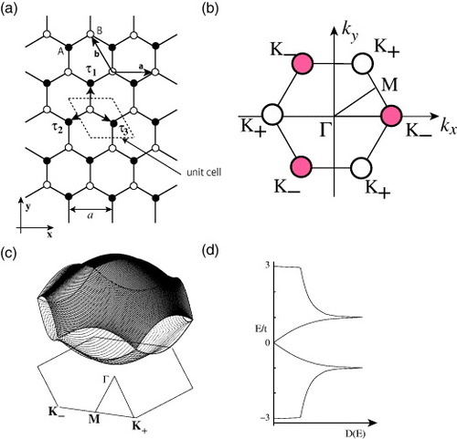
We start our discussion by reviewing the π-band structure of a graphene sheet [76]. Figures 1(a) and (b) show the lattice structure and the first Brillouin zone (BZ) of graphene, respectively. Graphene has a honeycomb lattice structure, and thus the first BZ is hexagonal. The corners of the first BZ are called K_± points, or Dirac points, because the low-energy spectrum at the corners can be described by the massless Dirac equation.

Figure 1 (a) Graphene sheet in real space, where the black (white) circles mean an A(B)-sublattice site; a is the lattice constant and a=(a, 0) and are the primitive vectors. Here , and . (b) First Brillouin zone of graphene. , , . (c) The π-band structure and (d) the density of states of a graphene sheet. The valence and conduction bands make contact at the degeneracy point K_±.

In this section, we employ a single-orbital nearest-neighbor tight-binding model for the π-electron network. The Hamiltonian can written as 1 where H.c. stands for the Hermitian conjugate; operators a^†_RA (b^†_RB) create and a_RA (b_RB) annihilate an electron at R_A (R_B) site of the A(B)-sublattice. These operators satisfy the Fermion anticommutation relations 2 3 and other combinations of anticommutation are zero; t is the transfer integral between nearest-neighbor carbon sites, which is roughly estimated as 3.0 eV in a graphene system. We apply the following Fourier transformation to the above Hamiltonian; 4 5 Here k= (k_x, k_y), and L_x(L_y) denotes the number of unit cells in the x(y)-direction. 6 Here we insert a one-particle state, 7 into the Schrödinger equation 8 Here |0〉 denotes the vacuum state. Note that α_k|0〉=β_k|0〉=0. Thus, we have 9 with 10 Thus, the energy bands are given by E_s=s|f_AB(k)|, namely, 11 with s=±1. Because one carbon site has one π-electron on average, only the E₋(k) band is completely occupied. The corresponding wavefunction can be written as 12 Thus, the Bloch wavefunction of graphene has phase and amplitude differences between A and B sublattice sites. This intrinsic phase structure determines many properties of graphene; it is the origin of the π-Berry phase around the Dirac K-points [4, 10] and of the chiral-dependent Klein tunneling [11]. As shown in the next section, this relative phase structure is preserved in the presence of an armchair edge; however, the presence of a zigzag edge has a detrimental effect. The DOS is calculated as 13 where the k-integration is taken over the first BZ, and η is an infinitesimally small real number.

Figures 1(c) and (d) depict the energy dispersion of π-bands in the first BZ and the corresponding DOS, respectively. Near the Γ point, both valence and conduction bands can be expressed as quadratic functions of k_x and k_y, i.e. E_k=±(3−3|k|²/4). At the M points, which are the midpoints of sides of the hexagonal first BZ, a saddle point appears in the energy dispersion, and the DOS diverges logarithmically. Near the K point at the corner of the hexagonal first BZ, the energy dispersion is a linear function of the magnitude of the wave vector, , where the DOS linearly depends on energy. Here, is the lattice constant. The Fermi energy is located at the K points, and there is no energy gap at these points because there E_k vanishes owing to the hexagonal symmetry.

Graphene nanoribbons and edge states

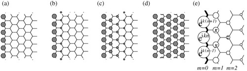
There are two types of a graphene edge; armchair and zigzag edges. These two edges have a 30° difference in their orientation within the graphene sheet. Here we briefly discuss the origin of the large difference in the π electronic structures induced by the two types of graphene edges [15]. In particular, a zigzag edge exhibits localized states, whereas an armchair edge does not induce such localized states.

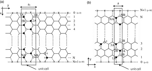
A simple and useful method of studying the edge and size effects is to use the graphene nanoribbon models shown in figures 2(a) and (b). We define the width of a graphene ribbon as N, where N is the number of dimer (two carbon sites) lines for the armchair nanoribbon and the number of zigzag lines for the zigzag nanoribbon. It is assumed that all dangling bonds at graphene edges are terminated by hydrogen atoms and thus do not contribute to the electronic states near the Fermi level. We employ a single-orbital tight-binding model for the π electron network. Details of the energy spectrum and wavefunction are given in the following subsection and in the appendices, and here we quickly overview the electronic states of graphene nanoribbons.

Figure 2 Structure of graphene nanoribbons with (a) armchair edges (armchair ribbon) and (b) zigzag edges (zigzag ribbon). The dashed rectangles define the unit cells; a_T and a are the respective unit cell widths for armchair and zigzag nanoribbons; N defines the ribbon width. The × marks indicate the missing carbon atoms for the edge boundary condition.

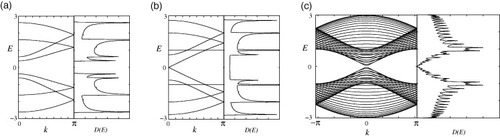
Figures 3(a)–(c) show the DOS and the energy band structures of armchair ribbons for three different ribbon widths. The wavenumber k is normalized by the length of the primitive translation vector of each graphene nanoribbon, and the energy E is scaled by the transfer integral t. The top of the valence band and the bottom of the conduction band are located at k=0. Note that the ribbon width determines whether the system is metallic or semiconducting. As shown in figure 3(b), the system is metallic when N=3M−1, where M is an integer. For semiconducting ribbons, the direct band gap decreases with increasing ribbon width and approaches zero in the limit of very large N. For narrow undoped metallic armchair nanoribbons, an energy gap can be formed by Peierls instabilities at low temperatures [77], which is consistent with density functional theory calculations [21, 35, 78].

Figure 3 Energy band structure E(k) and density of states D(E) of armchair ribbons of various widths: (a) N=4, (b) N=5 and (c) N=30. Adapted from [89].

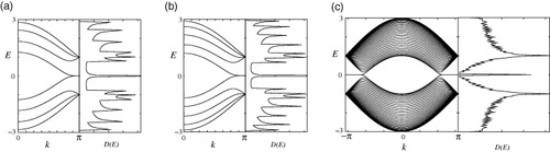
For zigzag ribbons, however, a remarkable feature arises in the band structure, as shown in figures 4(a)–(c). The top of the valence band and the bottom of the conduction band are always degenerate at k=π, and the degeneracy of the center bands at k=π does not originate from the intrinsic band structure of the graphene sheet. These two special center bands flatten with increasing ribbon width. A pair of partial flat bands appears within the region 2π/3≤|k|≤π, where the bands are located in the vicinity of the Fermi level.

Figure 4 Energy band structure E(k) and density of states D(E) of zigzag ribbons of various widths: (a) N=4, (b) N=5 and (c) N=30. Adapted from [89].

The electronic states in the partial flat bands of the zigzag ribbons can be understood as localized states near the zigzag edge by examining the charge density distribution [15–17, 22–24]. Here we show that the puzzling emergence of the edge states can be explained by considering a semi-infinite graphite sheet with a zigzag edge. First we show the distribution of charge density in flat band states for different wavenumbers in figures 5(a)–(d), where the amplitude is proportional to the circle radius. The wavefunction has a nonbonding character, i.e. it only has a finite amplitude on one of the two sublattices that include the edge sites. It is completely localized at the edge site when k=π and starts to gradually penetrate into the inner sites when k deviates from π, reaching an extended state at k=2π/3.

Figure 5 Charge density plot for analytical solution of the edge states in a semi-infinite graphene sheet for various wavenumber: (a) k=π, (b) k=8π/9, (c) k=7π/9 and (d) k=2π/3. (e) Analytical form of the edge state for a semi-infinite graphite sheet with a zigzag edge, shown by the bold lines. Each carbon site is specified by a location index n on the zigzag chain and by a chain order index m, which increases from the edge. The magnitude of the charge density at each site, such as x, y and z, is obtained analytically (see text). The radius of each circle is proportional to the charge density on each site, and the drawing corresponds to k=7π/9. Adapted from [89].

Considering the translational symmetry, we can start constructing the analytical solution for the edge state by letting the Bloch components of the linear combination of atomic orbitals (LCAO) wavefunction be …, e^ik(n−1), e^ikn, e^ik(n+1), … on successive edge sites, where n denotes a site located on the edge. Then, the mathematical condition necessary for the wavefunction to be exact for E=0 is that the sum of the components of the complex wavefunction over the nearest-neighbor sites becomes zero. In figure 5(e), the above condition implies that e^ik(n+1)+e^ikn+x=0, e^ikn+e^ik(n−1)+y=0 and x+y+z=0. Therefore, the wavefunction components x, y and z are found to be D_ke^ik(n+1/2), D_ke^ik(n−1/2) and D_k²e^ikn, respectively. Here, D_k=−2 cos(k/2). Thus, the charge density is proportional to D_k^2(m−1) at each non-nodal site of the mth zigzag chain from the edge. Then the convergence condition of |D_k|≤1 is required, for otherwise the wavefunction would diverge in a semi-infinite graphite sheet. This convergence condition defines the region 2π/3≤|k|≤π, where the flat bands appear.

The edge states are reasonably robust even if the graphene edge does not have a clear zigzag edge. Actually, a general edge structure that is not parallel to the armchair edge can have a zero-energy edge state, which was shown by using an analogy to the condition of the zero-energy Andreev bound state in an unconventional superconductor [73]. The robustness of edge states has been confirmed by numerical calculations [79]. Even for the armchair edge, a localized state and a complete flat band can be obtained in the case of a strong imbalance of the on-site potential energy between sublattice sites A and B [42]. The existence of edge states crucially affects the physical properties of nanographene systems as shown below.

Energy spectrum and wavefunctions

The entire energy spectrum and the wavefunction can also be obtained by solving the equation of motion for the nearest-neighbor tight-binding model. In the appendices, we show how to derive them using simple wave mechanics techniques, and here we summarize the results.

Armchair nanoribbons

For an armchair nanoribbon with width N, the energy spectrum is given by 14 Here, s=±1 and ∊_p=2 cos(p). s=+1 (s=−1) corresponds to the conduction (valence) energy band. The transverse wavenumber p is determined through the edge boundary condition by 15

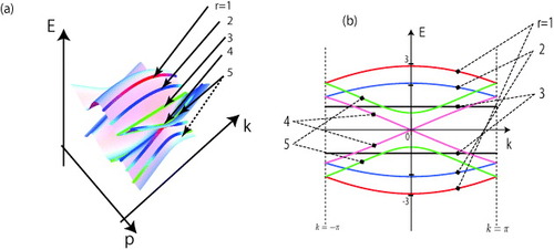
Figure 6(a) shows the energy surfaces given by equation (1414 ) for N=5 and discrete wavenumber p. Figure 6(b) is the corresponding projected energy band structure of a graphene nanoribbon with N=5. Note that E_s=0 at k=0 whenever N=3r−1 (r=1, 2, 3, …), which is simply the condition for metallic armchair nanoribbons. The energy band structures of armchair nanoribbons can be obtained by slicing the band structure of graphene, as in the case of carbon nanotubes [74, 75].

Figure 6 (a) 3D plot of bulk graphene band structure with translational invariance along the armchair axis (equation (1414 )) in the region of |k|π and |p|π. The bold lines correspond to the ribbon width N=5 and discrete transverse wavenumber p. (b) Energy band structure of armchair nanoribbon (N=5) with subband indexes, which is equivalent to the projection of the 3D plot onto the E−k plane; t and a_T are set equal to unity.

The wavefunction is written as 16 Here N_c is the normalization constant, which is explicitly derived in appendix A.

Zigzag nanoribbons

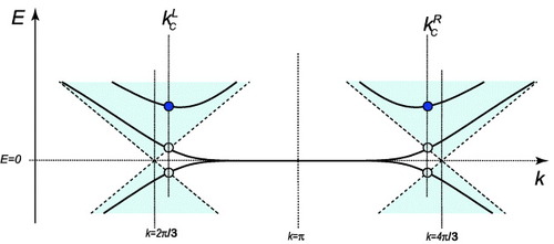
Zigzag nanoribbons have partially flat bands owing to the edge states, and thus we must discriminate between extended states and localized states; these states depend on the wavenumber k. As shown in figure 7, the energy spectrum for zigzag nanoribbons of width N has N extended eigenstates if E>0 and 0kk^L_c; however, it has N−1 extended eigenstates and a localized edge state if E>0 and k^L_ckπ, where k_c is given by 17

Figure 7 Schematic energy band dispersion near E=0 for zigzag nanoribbons. The bold lines indicate the energy subband of zigzag nanoribbons. The shaded area indicates the bulk graphene spectrum. Here t and a are set to unity.

The energy spectrum of zigzag nanoribbons for extended states can be given by 18 where s=±1 and g_k=2 cos(k/2). The transverse wavenumber p=p(k,N) is given as the solution of the equation 19 There are N solutions for p if 0kk^L_c or k^Rk2π but only (N−1) solutions if k^L_c<k<k^R. Since p depends not only on the ribbon width N but also on the longitudinal wavenumber k, we cannot obtain the energy band structures of zigzag nanoribbons simply by slicing the graphene band structure as in the case of armchair nanoribbons.

The wavefunction can be written as 20 with the normalization constant N_c.

The missing state corresponds to the edge state, which can be obtained by analytical continuation, i.e. p→π±iη for k_c^L<k<π, and p→0±iη for π<k<k_c^R. The corresponding energy spectrum is given as 21 and η is determined through the relation 22 The wavefunction for edge states is 23 where the normalization constant N_c is explicitly derived in appendix B.

Note that the wavefunction for armchair nanoribbons given by equation (1616 ) has a phase difference between sublattice sites A and B due to the chiral nature of graphene. On the other hand, the wavefunction for zigzag nanoribbons is always real and thus has no phase, irrespective of whether the state is extended or localized. This difference in wavefunctions between armchair and zigzag nanoribbons is related to the nature of pseudospin in graphene [80], and to some physical properties such as Kohn anomalies [81] and their effect on Raman scattering [82].

Energy band gap

Next we analytically show that both the energy gap Δ_a at k=0 for armchair ribbons and the energy gap Δ_z at k=2π/3 for zigzag ribbons are inversely proportional to the width of the graphite ribbon. This result indicates that the physical quantities related to the energy gap can be scaled by the ribbon width.

Armchair nanoribbons

As the direct gap always appears at k=0, we obtain E_s=s(1+∊_p) from the analytical solution given in the previous subsection. Thus, the energy gap Δ_a is given by 24 where m=1, 2, 3, ⋅⋅⋅. After expressing N in terms of , which is the ribbon width in the unit of the lattice constant a, and performing the Taylor expansion under the condition of 1/W≪1, we obtain the following results: 25 Thus, Δ_a is inversely proportional to the ribbon width.

Zigzag nanoribbons

Because in zigzag ribbons two states are degenerate at k=π, the gap of the zigzag ribbons is always zero and the system is always metallic. However, the energy bands have a gap at k=2π/3, because the bonding and antibonding configurations between the two edge states originating from both edges develop toward k=2π/3 from k=π. According to the projection of the band structure of a graphite sheet onto the first BZ of zigzag ribbons, the degenerate points of the valence and conduction bands of a graphene sheet meet at k=2π/3. Thus, in the limit of infinite ribbon width, the energy gap Δ_z at k=2π/3 is zero. The Hamiltonian of zigzag ribbons at k=2π/3 is rewritten as 26 which is equivalent to the tight-binding model for a one-dimensional lattice having 2N sites. The site index i corresponds to iA, if i is an odd number, and to iB, if i is an even number. The eigenvalues are evaluated as ∊=−2t cos(nπ/(2N+1)) (n=1, 2, …, 2N), and the corresponding eigenfunction at the jth site, Ψ_j, is Ψ_j=B sin (njπ/2N+1), where B is the normalization factor. Therefore, Δ_z is given as 27 A Taylor expansion under the condition of 1/N≪1 yields 28 Here, W=3N/2−1 is the ribbon width in the unit of the lattice constant. Thus, Δ_a is also inversely proportional to the ribbon width.

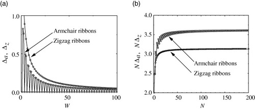
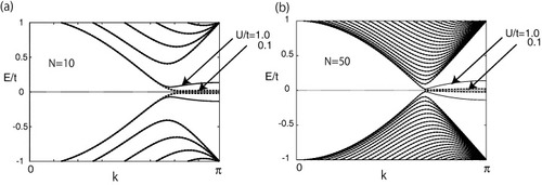
Figure 8(a) shows the width dependence of the energy gap for armchair and zigzag ribbons and figure 8(b) shows a plot of NΔ versus N. NΔ becomes constant for values greater than about N=30 (N=60) for zigzag (armchair) ribbons.

Figure 8 (a) Width dependence of the energy gap of armchair ribbons at k=0 (Δ_a) and zigzag ribbons at k=2π/3 (Δ_z). (b) Plot of NΔ_a and NΔ_z versus N. Adapted from [19].

Electronic transport properties

When the phase coherence length is larger than the system size, the electrical conductance of the system can be evaluated with the Landauer formula. In general, electron scattering in a quantum wire is described by a scattering matrix [83]. Through the scattering matrix S, the amplitudes of the scattered waves O are related to the incident waves I as 29 Here, r and r′ are reflection matrices, t and t′ are transmission matrices, and L and R denote the left and right lead lines, respectively. The Landauer–Büttiker formula [84] relates the scattering matrix to the conductance of the sample as 30 For simplicity, throughout this review we evaluate the electronic conductance in the unit of quantum conductance (e²/πℏ), i.e. as dimensionless conductance g(E).

Since the transmission probability is unity in the clean limit, the dimensionless conductance at zero temperature is equal to the number of channels, i.e. the number of subbands across the Fermi energy. Thus, the dimensionless conductance is given as 31 where n=0, 1, 2, ….

Graphene nanoribbons can be viewed as a new class of quantum wires. Thus, one might expect that random impurities inevitably cause Anderson localization, i.e. conductance decays exponentially with increasing system length L and vanishes in the limit of L→∞. In zigzag nanoribbons, however, subbands with partially flat bands appear owing to the edge states, which produce chiral modes separately in two valleys. There are two such modes with opposite orientation in each of the two valleys, which are well separated in k-space. It has been shown that such a chiral propagating mode provides a perfectly conducting channel, i.e. the zigzag nanoribbons with long-range impurities do not show Anderson localization [72]. This mechanism of the perfectly conducting channel is suppressed if intervalley scattering prevails due to the presence of strong short-range impurities such as in the case of a large concentration of vacancies and the strong fluctuation of ribbon width by random rough-edge structures [72]. In such a situation, zero-conductance Fano resonances appear in the low-energy transport regime, resulting in perfect backward scattering [85, 86].

On the other hand, the low-energy spectrum of armchair nanoribbons is described as the superposition of two nonequivalent Dirac points of graphene. In spite of the lack of two well-separated valleys, the single-channel transport in the presence of long-range impurities is nearly perfectly conducting, and the backward-scattering matrix elements vanish at the lowest order owing to the internal phase structure of the wavefunction [87]. More precisely, the backward-scattering matrix elements vanish at the lowest order close to the edge region, and they vanish at all orders in the bulk. This nearly perfect conduction mechanism in the metallic armchair nanoribbons can also be interpreted as the manifestation of a nontrivial Berry π phase for the single-channel linear band originating from the Dirac spectrum [88]. For a multichannel energy regime, however, conventional exponential decay of the average conductance occurs. The perfectly conducting channel might be the origin of the robust conduction mechanism of zigzag nanoribbons, in contrast to armchair nanoribbons [89–94].

Magnetic instability

The presence of a sharp peak in the DOS should induce lattice distortion via the electron–phonon interaction and/or magnetic polarization via the electron–electron interaction. Because of the nonbonding character of the edge states, lattice distortion in the vicinity of zigzag edges is unlikely, with the expected strength of the electron–phonon coupling [77]. The absence of lattice distortion was also confirmed by a density functional theory approach [20, 78]. Thus, we examine the effect of the electron–electron interaction using the Hubbard model with the unrestricted Hartree–Fock (HF) approximation. Here we find the possibility of spontaneous magnetic ordering near the edge, peculiar to nanometer-scale fragments of graphite.

The Hamiltonian is written as 32 where the operator c^†_{i, s} creates an electron with spin s on site i, and n_{i, s}=c^†_{i, s}c_{i, s}. The indexes of the sites in graphite ribbons are depicted in figures 2(a) and (b). The parameters t and U are the nearest-neighbor transfer integral and on-site Coulomb repulsion, respectively; 〈⋅⋅⋅〉 denotes the expectation value in the HF state. We solve the unrestricted HF Hamiltonian with the self-consistent conditions, i.e. , where m_i denotes the magnetic moment at site i in the unit of the Bohr magneton.

Figure 9 shows the U dependence of magnetization m for zigzag ribbons of N=2 (a), 3 (b) and 10 (c). The dashed lines are HF solutions for a 2D graphite sheet. Figure 10 shows the corresponding results for armchair ribbons of N=3 (a), 4 (b) and 5 (c). A peculiar feature of the zigzag ribbons is that large magnetic moments emerge on the edge carbon atoms, even for a small U, which is explained as follows: 2D graphite is a zero-gap semiconductor with DOS equal to zero at the Fermi level, and thus the slope of the broken line rapidly increases at U=U_C. This is consistent with the fact that graphite is nonmagnetic; thus, U is expected to be much smaller than t. On the other hand, the zigzag ribbons have a large DOS at the Fermi level originating from the edge states. Thus, nonzero magnetic solutions can emerge for infinitesimally small U as indicated in the present mean-field result. However, special emphasis should be placed on the behavior of the magnetization at edge site 1A. As shown in figure 9, the magnetization at the site 1A rapidly increases with the ribbon width and reaches about 0.2, even at small U≈0.1.

Figure 9 U dependence of the magnetization m for zigzag ribbons with (a) N=2, (b) N=3 and (c) N=10. The dashed lines correspond to the mean-field solutions for the graphite sheet. Adapted from [19].

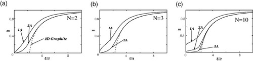
Figure 10 U dependence of the magnetization m for armchair ribbons with (a) N=3, (b) N=4 and (c) N=5. The dashed lines correspond to the mean-field solutions for the graphite sheet. Adapted from [19].

Note that the armchair ribbons do not show such singular magnetic behavior as shown in figures 10(a)–(c).

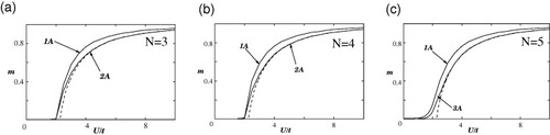
Next, we focus on the local ferrimagnetic structure of zigzag ribbons. We present the magnetic structure of the ribbon with N=10 at U/t=0.1 in figure 11(a), where spin alignment is visible at both edge sites. The origin of this structure can also be explained from the nature of the edge states, which are responsible for the magnetization. The amplitude of the edge state is nonzero only on one of the two sublattices at an edge and decreases in the inward direction. Thus, the magnetic moment selectively increases on this sublattice forming a local ferrimagnetic spin configuration, whereas it rapidly decreases at the inner sites. The opposite edge sites, however, belong to different sublattices, and the total magnetization of the zigzag graphite ribbon is zero, although the vanishing total spin for the ground state is consistent with the exact statement of the half-filled Hubbard model [95]. Figure 11(b) shows the dependence of magnetization at the outermost site (1A or NB) on the ribbon width N. Magnetization rapidly increases with the ribbon width and then saturates at approximately N=10. The energy band structure is shown in figure 12 for U/t=0.1 and 1.0 and N=10 (a) or 50 (b). Since the edge states are responsible for the edge spin polarization, the energy band gap does not uniformly open in the region 2π/3≤|k|≤π, i.e. the band gap is larger near k=π than near k=2π/3. The order of the energy band gap at k=π is about Um/t. Consequently, the corresponding spin wave modes become unconventional [18].

Figure 11 (a) Schematic magnetic structure of the zigzag ribbon with N=10 at U/t=0.1. (b) Dependence of the magnetization at the outermost site (1A) on the ribbon width N. The magnetization at site NB has the same magnitude but opposite sign to that at site 1A. Adapted from [19].

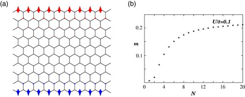
Figure 12 Energy dispersion for zigzag nanoribbons with (a) N=10 and (b) N=50 when U/t=0.1 and 1.0.

The ferrimagnetic spin polarizations along the zigzag edges are interesting from the viewpoint of the magnetic properties of nanographites. Nevertheless, the long-range order derived from the mean-field calculation is spurious, because no finite-momentum long-range spin order is expected in a one-dimensional system with full spin-rotation symmetry [96]. We may even argue that a quasi-long-range order, similar to that of the spin-1/2 Heisenberg chain, is not realized in zigzag ribbons of any finite width because the unit cell of the ribbons contains an even number of sites; thus, Haldane's conjecture applies, i.e. the system should exhibit a spin gap [97]. This is very similar to the case of ladder systems with an even number of legs, which display a resonating valence bond ground state, i.e. a short range correlated spin-liquid state. With increasing ribbon width, however, random phase approximation analysis shows that the spin gap Δ_s decreases exponentially owing to the diminished overlap between the two edges [18]. This means that zigzag edges favor spin polarization with the ferromagnetic alignment. Thus, a systematic analysis of the topological networks in nanographenes or nanographites will provide helpful guidelines for designing the new magnetic carbon materials [26, 32, 43, 44, 98, 99].

Summary

In this review, we have briefly introduced nanoscale effects on the electronic, transport and magnetic properties of graphene. Starting from basic facts about the electronic states of graphene, we have discussed how the electronic structures are modified as a result of the existence of the graphene edge by analyzing the electronic structures of graphene nanoribbons. We have shown that the analytical solution of the nearest-neighbor tight-binding model for graphene nanoribbons can be obtained in a simple and intuitive manner. Energy band structures of armchair nanoribbons were obtained by making the transverse wavenumber discrete, in accordance with the edge boundary condition. The electronic states are analogous to the case of carbon nanotubes [74, 75]. However, in zigzag nanoribbons the transverse wavenumber depends not only on the ribbon width N but also on the longitudinal wavenumber k, and thus the energy band structure cannot be obtained simply by slicing the bulk graphene band structure. The wavefunctions for armchair nanoribbons have a phase difference between A and B sublattice sites owing to the chiral nature of graphene; however, zigzag nanoribbons do not have such internal phase structures, i.e. their wavefunction is real irrespective of whether the state is extended or localized. This essential difference due to the edge orientation has a decisive effect on the transport, magnetic and optical properties of nanoscale graphene.

Acknowledgment

This work was financially supported by a Grant-in-Aid for Scientific Research (No. 20001006) from the Ministry of Education, Culture, Sports, Science and Technology (MEXT), Japan.

Appendix A Armchair nanoribbons

In this section, we outline a solution of the eigenvalue problem for armchair graphene nanoribbons (see figure 2(a)). The tight-binding Hamiltonian for armchair nanoribbons can be explicitly written as A.1 A.2 where a^†_l(m) and b^†_l(m) are the creation operators of an electron at the mA and mB sites in the lth unit cell, respectively. Similarly, a_l(m) and b_l(m) are the corresponding annihilation operators. The first line in the Hamiltonian represents the longitudinal hopping of electrons along the y-axis, and the second line describes the transverse hopping. The operators must satisfy the anticommutation relations A.3 A.4 and other anticommutations are zero. We have assumed that the system has L_y unit cells and the periodic boundary condition along the y-axis, i.e. A.5 Hereafter, the width of the unit cell a_T and the transfer integral are set to 1, for simplicity.

To derive the equations of motion, we apply the Fourier transformation to the tight-binding Hamiltonian along the translationally invariant y-axis, A.6 A.7 where y_{l, mA} (y_{l, mB}) is the y-coordinate of the mA (mB) site in the lth unit cell. To be precise, the y-coordinates of mA and (m+1)B (m=1, 2, 3, …) are not identical, and differ by a_cc/2 (a_cc() is the C–C bond length) due to the honeycomb lattice structure. Since the extra phase due to such a difference can be absorbed into the wavefunctions, we define the y-coordinates for the carbon sites in the unit cell as A.8 A.9

Because we use the periodic boundary condition along the y-axis, i.e. e^ikL_y=1, from the fact that a_l+Ly(m)=a_l(m) and b_l+Ly(m)=b_l(m), the longitudinal wavenumber k is given by A.10 In graphene nanoribbons, one can assume that L_y is infinite and k is continuous. However, it is worth noting that the electronic states of armchair nanotubes with finite length N and its circumstance L_ya_T can be analytically obtained if we assume that L_y has a finite value. The case of the open boundary condition in the longitudinal direction was recently studied using the monomer Green's function approach [100, 101].

Here we define the one-particle state A.11 where |0〉 denotes a vacuum state. Note that α_k(m)|0〉=β_k(m)|0〉=0. Inserting this one-particle state into the Schrödinger equation A.12 we obtain the following set of equations of motion: A.13 A.14 where m=1, 2, 3, …, N. The range of the wavenumber is −π≤k≤π. However, since the 0B, 0A, (N+1)A and (N+1)B sites are missing, the equations of motion are modified at the armchair edge to A.15 A.16 A.17 A.18 Thus, we assume the boundary condition for armchair nanoribbons as A.19 To solve the equations of motion, we assume that the generic solutions for ψ_{m, A} and ψ_{m, B} have the form A.20 A.21 Here A, B, C and D are arbitrary coefficients, which will be determined under the above boundary condition; p is the wavenumber in the transverse direction, which is also given by the boundary condition. From the boundary condition, we have the following relations: A.22 A.23 A.24 A.25 where z=e^ip(N+1). Thus, we have A.26 A.27 Substituting these functions into the equations of motion, we obtain the relation A.28 where ∊_p=2 cos(p). The condition for a nontrivial solution for A and C, i.e. A.29 is A.30 Then, we immediately obtain the solution for the eigenenergy as A.31 Here, s=±1, and s=+1 (s=−1) corresponds to the conduction (valence) energy band.

We can set the condition for the transverse wavenumber p as follows. Since the boundary condition yields z⁻¹B=−zA and B=−A, we have B=−z²A=z²B, i.e. z²=e^i2p(N+1)=1. Therefore, A.32 Note that E_s=0 at k=0 whenever N=3r−1 (r=1, 2, 3, …), which is simply the condition for metallic armchair nanoribbons.

The wavefunction is written as A.33 Here N_c is the normalization constant, which satisfies the equation A.34 A simple calculation yields A.35 then we have A.36

The real-space wavefunction (Ψ_{m, A}(y_{l, mA}), Ψ_{m, B}(y_{l, mB})) can be obtained by the Fourier transform of (ψ_{m, A}, ψ_{m, B}), defined in a similar manner to equation (A.7A.37 ). Thus, A.37

Further remarks can be made for the case of a semi-infinite graphene sheet with an armchair edge. Since the boundary condition ψ_{N+1, A}=ψ_{N+1, B}=0 is used only for determining the transverse wavenumber p (see equation (A.32A.32 )), the electronic states of a semi-infinite graphene sheet with an armchair edge can be obtained simply by removing this condition and by treating p as a continuous variable. This result is consistent with the results of studies using a continuous model [80, 102].

Appendix B Zigzag nanoribbons

In this section, we outline a solution of the eigenvalue problem for zigzag graphene nanoribbons (see figure 2(b)). The tight-binding Hamiltonian for zigzag nanoribbons can be explicitly written as B.1 B.2 where a^†_l(m) and b^†_l(m) are the creation operators of an electron at the mA and mB sites in the lth unit cell, respectively. Similarly, a_l(m) and b_l(m) are the corresponding annihilation operators. The first line in the Hamiltonian represents the longitudinal hopping of electrons along the x-axis, and the second line describes the transverse hopping. The operators must satisfy the anticommutation relations B.3 B.4 and other anticommutations are zero. We have assumed that the system has L_y unit cells. Similarly to the case of armchair ribbons, the lattice constant a and the transfer integral are set to 1 for simplicity.

To derive the equations of motion, we apply the Fourier transformation to the tight-binding Hamiltonian along the translationally invariant x-axis, B.5 B.6 where x_{l, mA} (x_{l, mB}) is the x-coordinate of the mA (mB) site in the lth unit cell. Because we have used the periodic boundary condition along the x-axis, i.e. e^ikL_x=1, from the fact that a_l+Lx(m)=a_l(m) and b_l+Lx(m)=b_l(m), the transverse wavenumber k is given by B.7 In graphene nanoribbons, one can assume that L_x is infinite and k is continuous. However, it is worth noting that the electronic states of zigzag nanotubes with finite length N and its circumstance L_xa can be analytically obtained if we assume that L_x shas a finite value.

Here we define the one-particle state B.8 where |0〉 denotes a vacuum state. Note that α_k(m)|0〉=β_k(m)|0〉=0. Inserting this one-particle state into the Schrödinger equation B.9 we obtain the following set of equations of motion: B.10 B.11 Here g_k=2 cos(k/2), and the site index m=0, 1, 2, …, N+1. However, since the 0B and (N+1)A sites are missing, the equations of motion are modified at the zigzag edge site to B.12 B.13 Thus, we give the boundary condition for zigzag nanoribbons as ψ_{0, B}=ψ_{N+1, A}=0.

We assume the generic solution for ψ_{m, A} and ψ_{m, B} to be B.14 B.15 Here A, B, C and D are arbitrary coefficients, which will be determined under the above boundary condition; p is the wavenumber in the transverse direction, which is also given by the boundary condition.

From the boundary condition, we have the following relations: B.16 B.17 where z=e^ip(N+1). Thus, we have B.18 B.19 Substituting these functions into the equations of motion, we obtain the relation B.20 with B.21 The condition for a nontrivial solution for A and C, i.e. (A, C)^T≠0, is det M=0. However, note that the solutions of p=0 and ±π should be excluded as unphysical because matrix M becomes zero for these values of p. In other words, such values yield ψ_{m, A}=ψ_{m, B}=0 for arbitrary m, i.e. electrons are absent in the system. Therefore, we can find solutions that satisfy det M=0 for arbitrary m except when p=0, ±π. After some arithmetic, we can show that det M=0 has the following form: B.22 where v, w and x are functions of E, g_k and z. Thus, all the coefficients of e^±i2pm terms and the constant term should be equal to zero. From the coefficient of e^±i2pm, we obtain the energy spectrum B.23 Thus, the energy eigenvalue is B.24 where s=±1, and s=+1 (s=−1) corresponds to the conduction (valence) energy band. Similarly, from the condition that the constant term should also be equal to zero, B.25 which yields the condition for the transverse wavenumber p. Substituting equation (B.23B.23 ) into equation (B.25B.25 ) to eliminate E², we obtain B.26 This equation yields the transverse wavenumber p=p(k,N), which is, however, not a simple form as in the case of armchair nanoribbons. The transverse wavenumber depends not only on the width N but also on the longitudinal wavenumber k. These properties of p can be also observed using the approach of the massless Dirac equation [19, 103].

We can obtain the relation C=−Az from the parity of the zigzag nanoribbon, i.e. ψ_{N+1−m, A}=ψ_{m, B}, and thus the generic form of the wavefunction can be written as B.27 with the normalization constant N_c.

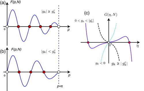
We now closely inspect the analytic properties for the condition F(p,N)=0, which determines the transverse wavenumber p for a given g_k. As F(p, N) is a periodic odd function, i.e. F(p+2π,N)=F(p,N) and F(−p,N)=−F(p,N), it is sufficient to search for the solutions within the range 0<p<π.

B.1 Extended states

Figure B1 schematically shows F(p, N) for (a) |g_k|≥g_k^c and (b) |g_k|<g_k^c in the case of N=4. Let us define the solutions F(p,N)=0 for fixed N as p_i (i=1, 2, …, p_n) within 0<p<π, i.e. excluding p=0, π. All these p_i solutions give the extended states. The number of p_i depends on the value of g_k, B.28 As shown below, g^c_k depends on the ribbon width N and becomes g^c_k∼1 for N≫1; g^c_k is analytically given as B.29 and can be written explicitly as B.30 Using the relation g_k=2 cos(k/2), we can obtain the critical k_c that yields g^c_k as B.31 In general, there are two solutions k_c(=k^L_c, k^R_c) within 0kπ as shown in figure 7. In the limit of large N, g_c=±1, and k_c^L=2π/3 and k_c^R=4π/3, which correspond to the Dirac K_± points.

Figure B1 Schematic figure of F(p, N) for (a) |g_k|≥g_k^c and (b) |g_k|<g_k^c in the case of N=4. Note that p=0 and π (empty circles) are unphysical solutions. There are N (4 filled circles) solutions corresponding to extended states for |g_k|≥g_k^c, but only N−1 (3 filled circles) solutions corresponding to extended states (filled circles) for |g_k|<g_k^c. The missing state corresponds to edge states, which can be found as the nonzero η-solution of G(η,N)=0 shown in (c). Note that the η=0 solution (empty circle) is unphysical. Nonzero η-solutions (filled circles) can appear for 0<g_k<|g_k^c|.

The wavefunction for extended states is written as B.32 with the normalization constant N_c, where B.33 B.34

The real-space wavefunction (Ψ_{m, A}(x_{l, mA}), Ψ_{m, B}(x_{l, mB})) can be obtained by the Fourier transform of (ψ_{m, A}, ψ_{m, B}), which is defined in a similar manner to equation (B.6B.6 ). Thus, B.35

B.2 Edge states

As we can see from equation (B.28B.28 ), one solution is missing for |g_k|≥g^c_k. This solution can be obtained by analytical continuation as B.36 B.37 The transverse imaginary wavenumber that damps the wavefunction toward the inner sites is given by the following relation: B.38 Each of them yields a single η solution corresponding to the edge state. B.39 Figure B1(c) schematically shows G(η,N) in the case of N=4. One can see that G(η,N) has a nonzero η solution if 0<g_k<|g_k^c|.

After analytical continuation, we can obtain the wavefunction for the edge states as B.40 and B.41 with a common normalization constant N_c, B.42 B.43

The real-space wavefunction (Ψ_{m, A}(x_{l, mA}), Ψ_{m, B}(x_{l, mB})) can be given by B.44 and B.45

The equation of motion for zigzag nanoribbons (equation (B.11B.11 )) can be rewritten by eliminating ψ_{m, B} to obtain the recurrence relation with three terms [17, 104, 105]: B.46 with a=E²−1−g_k² and b=−g_k, and we can solve this equation directly, provided we have the edge boundary condition [105]. On the other hand, the equation of motion for armchair nanoribbons can be expressed as a five-term recurrence equation [17], and its solution cannot be easily obtained. Our wave mechanics approach and the boundary condition for armchair nanoribbons might include some hidden symmetry to avoid this problem. A discussion of this case will be published elsewhere.

References

- NovoselovK SGeimA KMorozovS VJiangDZhangYDubonosS VGrigorievaI VFirsovA A 2004 Science 306 666 http://dx.doi.org/10.1126/science.1102896
- GeimA KNovoselovK S 2007 Nat. Mater. 6 183 http://dx.doi.org/10.1038/nmat1849
- Castro NetoA HGuineaFPeresN MNovoselovK SGeimA K 2009 Rev. Mod. Phys. 81 109 http://dx.doi.org/10.1103/RevModPhys.81.109
- AndoT 2005 J. Phys. Soc. Japan 74 777 http://dx.doi.org/10.1143/JPSJ.74.777
- AndoT 2008 Prog. Theor. Phys. Suppl. 176 203 http://dx.doi.org/10.1143/PTPS.176.203
- NovoselovK SGeimA KMorozovS VJiangDKatsnelsonM IGrigorievaI VDubonosS VFirsovA A 2005 Nature 438 197 http://dx.doi.org/10.1038/nature04233
- ZhangYTanY WStormerH LKimP 2005 Nature 438 201 http://dx.doi.org/10.1038/nature04235
- NovoselovK SMcCannEMorozovS VFal'koV IKatsnelsonM IZeitlerUJiangDSchedinFGeimA K 2006 Nat. Phys. 2 177 http://dx.doi.org/10.1038/nphys245
- AndoTNakanishiT 1998 J. Phys. Soc. Japan 67 1704 http://dx.doi.org/10.1143/JPSJ.67.1704
- AndoTNakanishiTSaitoR 1998 J. Phys. Soc. Japan 67 2857 http://dx.doi.org/10.1143/JPSJ.67.2857
- KatsnelsonM INovoselovK SGeimA K 2006 Nat. Phys. 2 620 http://dx.doi.org/10.1038/nphys384
- Luk'yanchukI AKopelevichY 2004 Phys. Rev. Lett. 93 166402 http://dx.doi.org/10.1103/PhysRevLett.93.166402
- BolotinK ISikesK JJiangZKlimaMFudenbergGHoneJKimPStormerH L 2008 Solid State Commun. 146 351 http://dx.doi.org/10.1016/j.ssc.2008.02.024
- BalandinA AGhoshSBaoW ZCalizoITeweldebrhanDMiaoFLauC N 2008 Nano Lett. 8 902 http://dx.doi.org/10.1021/nl0731872
- FujitaMWakabayashiKNakadaKKusakabeK 1996 J. Phys. Soc. Japan 65 1920 http://dx.doi.org/10.1143/JPSJ.65.1920
- NakadaKFujitaMDresselhausGDresselhausM S 1996 Phys. Rev. B 54 17954 http://dx.doi.org/10.1103/PhysRevB.54.17954
- WakabayashiKFujitaMAjikiHSigristM 1999 Phys. Rev. B 59 8271 http://dx.doi.org/10.1103/PhysRevB.59.8271
- WakabayashiKSigristMFujitaM 1998 J. Phys. Soc. Japan 67 2089 http://dx.doi.org/10.1143/JPSJ.67.2089
- WakabayashiK 2000PhD Thesis University of Tsukuba http://www.tulips.tsukuba.ac.jp/dspace/handle/2241/2592
- SonY WCohenM LLouieS G 2006 Nature 444 347 http://dx.doi.org/10.1038/nature05180
- SonY MCohenM LLouieS G 2006 Phys. Rev. Lett. 97 216803 http://dx.doi.org/10.1103/PhysRevLett.97.216803
- KobayashiYFukuiKEnokiTKusakabeKKaburagiY 2005 Phys. Rev. B 71 193406 http://dx.doi.org/10.1103/PhysRevB.71.193406
- KobayashiYFukuiKEnokiT 2006 Phys. Rev. B 73 125415 http://dx.doi.org/10.1103/PhysRevB.73.125415
- NiimiYMatsuiTKambaraHTagamiKTsukadaMFukuyamaH 2006 Phys. Rev. B 73 085421 http://dx.doi.org/10.1103/PhysRevB.73.085421
- SugawaraKSatoTSoumaSTakahashiTSuematsuH 2006 Phys. Rev. B 73 045124 http://dx.doi.org/10.1103/PhysRevB.73.045124
- WakabayashiKHarigayaK 2003 J. Phys. Soc. Japan 72 998 http://dx.doi.org/10.1143/JPSJ.72.998
- YamashiroAShimoiYHarigayaKWakabayashiK 2003 Phys. Rev. B 68 193410 http://dx.doi.org/10.1103/PhysRevB.68.193410
- HarigayaKEnokiT 2002 Chem. Phys. Lett. 351 128 http://dx.doi.org/10.1016/S0009-2614(01)01338-0
- YoshiokaH 2003 J. Phys. Soc. Japan 72 2145 http://dx.doi.org/10.1143/JPSJ.72.2145
- KumazakiHHirashimaD S 2008 J. Phys. Soc. Japan 77 044705 http://dx.doi.org/10.1143/JPSJ.77.044705
- HikiharaTHuXLinH-HMouC-Y 2003 Phys. Rev. B 68 035432 http://dx.doi.org/10.1103/PhysRevB.68.035432
- KusakabeKMaruyamaM 2003 Phys. Rev. B 67 092406 http://dx.doi.org/10.1103/PhysRevB.67.092406
- PalaciosJ JFernández-RossierJBreyL 2008 Phys. Rev. B 77 195428 http://dx.doi.org/10.1103/PhysRevB.77.195428
- Fernández-RossierJPalaciosJ J 2007 Phys. Rev. Lett. 99 177204 http://dx.doi.org/10.1103/PhysRevLett.99.177204
- HodOBaroneVScuseriaG E 2008 Phys. Rev. B 77 035411 http://dx.doi.org/10.1103/PhysRevB.77.035411
- HodOBaroneVPeraltaJ EScuseriaG E 2007 Nano Lett. 7 2295 http://dx.doi.org/10.1021/nl0708922
- HodOPeraltaJ EScuseriaG E 2007 Phys. Rev. B 76 233401 http://dx.doi.org/10.1103/PhysRevB.76.233401
- EzawaM 2008 Physica E 40 1421 http://dx.doi.org/10.1016/j.physe.2007.09.031
- EzawaM 2007 Phys. Rev. B 76 245415 http://dx.doi.org/10.1103/PhysRevB.76.245415
- KundinK N 2008 ACS Nano 2 516 http://dx.doi.org/10.1021/nn700229v
- WassmannTSeitsonenA PSaittaMLazzeriMMauriF 2007 Phys. Rev. Lett. 101 096402 http://dx.doi.org/10.1103/PhysRevLett.101.096402
- WakabayashiKOkadaSTomitaRFujimotoSNatsumeY 2010 J. Phys. Soc. Japan 79 034706 http://dx.doi.org/10.1143/JPSJ.79.034706
- DuttaS 2009 Phys. Rev. Lett. 102 096601 http://dx.doi.org/10.1103/PhysRevLett.102.096601
- KanE 2008 J. Am. Chem. Soc. 130 42224
- HanM YÖzyilmazBZhangYKimP 2007 Phys. Rev. Lett. 98 206805 http://dx.doi.org/10.1103/PhysRevLett.98.206805
- ChenZLinY-MRooksM JAvourisP 2007 Physica E 40 228 http://dx.doi.org/10.1016/j.physe.2007.06.020
- LiXWangXZhangLLeeSDaiH 2008 Science 319 1229 http://dx.doi.org/10.1126/science.1150878
- JiaoLZhangLWangXDiankovGDaiH 2009 Nature 458 877 http://dx.doi.org/10.1038/nature07919
- KosynkinD VHigginbothamA LSinitskiiALomedaJ RDimievAPriceB KTourJ M 2009 Nature 458 872 http://dx.doi.org/10.1038/nature07872
- YangXDouXRouhanipourAZhiLRäderJMüllenK 2008 J. Am. Chem. Phys. 130 4216
- MolitorFGüttingerJStampferCGrafDIhnTEnsslinK 2007 Phys. Rev. B 76 245426 http://dx.doi.org/10.1103/PhysRevB.76.245426
- WangXOuyangYLiXWangHGuoJDaiH 2008 Phys. Rev. Lett. 100 206803 http://dx.doi.org/10.1103/PhysRevLett.100.206803
- TapasztoLDobrikGLambinPBiróL P 2008 Nat. Nanotech. 3 397 http://dx.doi.org/10.1038/nnano.2008.149
- StampferCGüttingerJHellmüllerEnsslinM KIhnT 2009 Phys. Rev. Lett. 102 056403 http://dx.doi.org/10.1103/PhysRevLett.102.056403
- MiyazakiH et al 2008 Appl. Phys. Express 1 024001 http://dx.doi.org/10.1143/APEX.1.024001
- GüttingerStampferCLibischFFreyTBurgdörfeJIhnTEnsslinK 2009 Phys. Rev. Lett. 103 046810 http://dx.doi.org/10.1103/PhysRevLett.103.046810
- JiaX et al 2009 Science 323 1701 http://dx.doi.org/10.1126/science.1166862
- CamposL CManfrinatoV RSanchez-YamgishiJ DKongJJarillo-HerreroP 2009 Nano Lett. 9 2600 http://dx.doi.org/10.1021/nl900811r
- CaiJ et al 2010 Nature 466 470 http://dx.doi.org/10.1038/nature09211
- WakabayashiKSigristM 2000 Phys. Rev. Lett. 84 3390 http://dx.doi.org/10.1103/PhysRevLett.84.3390
- WakabayashiK 2001 Phys. Rev. B 64 125428 http://dx.doi.org/10.1103/PhysRevB.64.125428
- WakabayashiKAokiT 2002 Int. J. Mod. Phys. B 16 4897 http://dx.doi.org/10.1142/S0217979202014917
- YamamotoMWakabayashiK 2009 Appl. Phys. Lett. 95 082109 http://dx.doi.org/10.1063/1.3206915
- RycerzATworzydloJBeenakkerC W J 2007 Nat. Phys. 3 172 http://dx.doi.org/10.1038/nphys547
- KaneC LMeleE J 2005 Phys. Rev. Lett. 95 226801 http://dx.doi.org/10.1103/PhysRevLett.95.226801
- HasanM ZKaneC L 2010 arXiv:1002.3895
- AkhmerovA RBeenakkerC W J 2008 Phys. Rev. B 77 205416 http://dx.doi.org/10.1103/PhysRevB.77.205416
- CrestiAGrossoGParraviciniP 2008 Phys. Rev. B 77 233402 http://dx.doi.org/10.1103/PhysRevB.77.233402
- NakabayashiJYamamotoDKuriharaS 2009 Phys. Rev. Lett. 102 066803 http://dx.doi.org/10.1103/PhysRevLett.102.066803
- WakabayashiKSigristM 2008 J. Phys. Soc. Japan 78 034717
- BeenakkerC W J 2006 Phys. Rev. Lett. 97 067007 http://dx.doi.org/10.1103/PhysRevLett.97.067007
- WakabayashiKTakaneYSigristM 2007 Phys. Rev. Lett. 99 036601 http://dx.doi.org/10.1103/PhysRevLett.99.036601
- WakabayashiKTakaneYSigristM 2009 Carbon 47 124 http://dx.doi.org/10.1016/j.carbon.2008.09.040
- SaitoRFujitaMDresselhausGDresselhausM S 1992 Phys. Rev. B 46 1804 http://dx.doi.org/10.1103/PhysRevB.46.1804
- SaitoRFujitaMDresselhausGDresselhausM S 1992 Appl. Phys. Lett. 60 2204 http://dx.doi.org/10.1063/1.107080
- WallaceP R 1947 Phys. Rev. 71 622 http://dx.doi.org/10.1103/PhysRev.71.622
- FujitaMIgamiMNakadaK 1997 J. Phys. Soc. Japan 66 1864 http://dx.doi.org/10.1143/JPSJ.66.1864
- MiyamotoYNakadaKFujitaM 1999 Phys. Rev. B 59 9858 http://dx.doi.org/10.1103/PhysRevB.59.9858
- WimmerMAkhmerovA RGuineaF 2010 Phys. Rev. B 82 045409 http://dx.doi.org/10.1103/PhysRevB.82.045409
- SasakiKWakabayashiK 2010 Phys. Rev. B 82 035421 http://dx.doi.org/10.1103/PhysRevB.82.035421
- SasakiKYamamotoMMurakamiSSaitoRDresselhausM STakaiKMoriTEnokiTWakabayashiK 2009 Phys. Rev. B 80 155450 http://dx.doi.org/10.1103/PhysRevB.80.155450
- SasakiKSaitoRWakabayashiKEnokiT 2010 J. Phys. Soc. Japan 79 044603 http://dx.doi.org/10.1143/JPSJ.79.044603
- BeenakkerC W J 1997 Rev. Mod. Phys. 69 731 http://dx.doi.org/10.1103/RevModPhys.69.731
- BüttikerMImryYLandauerRPinhasS 1985 Phys. Rev. B 31 6207 http://dx.doi.org/10.1103/PhysRevB.31.6207
- WakabayashiK 2002 J. Phys. Soc. Japan 71 2500 http://dx.doi.org/10.1143/JPSJ.71.2500
- Zar∘boL PNikolićB K 2007 Europhys. Lett. 80 47001 http://dx.doi.org/10.1209/0295-5075/80/47001
- YamamotoMTakaneYWakabayashiK 2009 Phys. Rev. B 79 125421 http://dx.doi.org/10.1103/PhysRevB.79.125421
- SasakiKWakabayashiKEnokiT 2010 New J. Phys. 12 083023 http://dx.doi.org/10.1088/1367-2630/12/8/083023
- WakabayashiKTakaneYYamamotoMSigristM 2009 New J. Phys. 11 095016 http://dx.doi.org/10.1088/1367-2630/11/9/095016
- LiT CLuS P 2008 Phys. Rev. B 77 085408 http://dx.doi.org/10.1103/PhysRevB.77.085408
- LouisEVergésJ AGuineaFChiappeG 2007 Phys. Rev. B 75 085440 http://dx.doi.org/10.1103/PhysRevB.75.085440
- MuccioloE RCastro NetoA HLewenkopfC H 2009 Phys. Rev. B 79 075407 http://dx.doi.org/10.1103/PhysRevB.79.075407
- AreshkinD AGunlyckeDWhiteC T 2007 Nano Lett. 7 204 http://dx.doi.org/10.1021/nl062132h
- CrestiARocheS 2009 New J. Phys. 11 095004 http://dx.doi.org/10.1088/1367-2630/11/9/095004
- LiebE H 1989 Phys. Rev. Lett. 62 1201 http://dx.doi.org/10.1103/PhysRevLett.62.1201
- PitaevskiiLStringariS 1991 J. Low. Temp. Phys. 85 377 http://dx.doi.org/10.1007/BF00682193
- DagottoERiceT M 1996 Science 271 618 http://dx.doi.org/10.1126/science.271.5249.618
- MakarovaT L 2004 Semiconductors 38 615 http://dx.doi.org/10.1134/1.1766362
- OkadaSOshiyamaA 2001 Phys. Rev. Lett. 87 146803 http://dx.doi.org/10.1103/PhysRevLett.87.146803
- OnipkoA 2008 Phys. Rev. B 78 245412 http://dx.doi.org/10.1103/PhysRevB.78.245412
- MalyshevaLOnipkoA 2008 Phys. Rev. Lett. 100 186806 http://dx.doi.org/10.1103/PhysRevLett.100.186806
- SakaiKTakaiKFukuiKNakanishiTEnokiT 2010 Phys. Rev. B 81 235417 http://dx.doi.org/10.1103/PhysRevB.81.235417
- BreyLFertigH A 2006 Phys. Rev. B 73 235411 http://dx.doi.org/10.1103/PhysRevB.73.235411
- RammalR 1985 J. Physique 46 1345 http://dx.doi.org/10.1051/jphys:019850046080134500
- SasakiKMurakamiSSaitoR 2006 Appl. Phys. Lett. 88 113110 http://dx.doi.org/10.1063/1.2181274