Abstract
A new mechanism based on the effect of local magnetic forces on diffusing ions around a growing ferromagnetic precipitate is proposed. A 3D simulation based only on physical parameters is undertaken in which main assumption is of interface limited growth controlled by the effect of both curvature and local magnetic field distortion. Although usually neglected in magnetic field effect mechanisms, it is shown that these local magnetic forces acting on a single paramagnetic ion can change markedly affect the growth process and induce strong shape anisotropy.
Introduction
In binary alloys such as Co-rich eutectic systems, a magnetic phase exhibits a ferromagnetic transition at a high temperature which may even be very close to the solidification point [Citation1]. If solidification or heat treatments are performed under a strong external magnetic field, it is thus expected that the magnetic interactions will affect the growth of the magnetic phase and will lead to the formation of new microstructures. In the case of solidification, it has been observed that Co-rich phases form structures elongated parallel to the external applied field [Citation1, Citation2]. In the case of high-temperature annealing under magnetic field, the growth of the phases is anisotropic and aligned along the field direction [Citation2].
Several mechanisms are known to affect the structure of materials under a magnetic field. A magnetic torque can rotate elongated particles and align them along the field direction. The mechanism expected for the rotation of a solid phase in a liquid may also be expected for the rotation of a precipitate in a matrix if sufficient time is allowed for creep in the matrix. Similarly, magnetic phases are expected to elongate along the field direction due to the effect of a demagnetizing field. This effect is known on the free surfaces of ferrofluids, which form elongated spikes under low external magnetic fields, and should also be expected for highly magnetic solid phases if sufficient time is allowed for creep due to atomic diffusion in the solid state.
The effects of both torque and demagnetizing are related to the phase magnetization itself and should saturate once the magnetization becomes saturated However, it was experimentally observed that the shape elongation of precipitates due to solid-state growth was not saturated in fields between 7 and 16 T, although the magnetization itself was expected to have been saturated in much lower fields [Citation2]. In addition to the standard texturing mechanisms that may account for the observed structure, such as the magnetic orientation and deformation due to demagnetizing energy, the local effect of magnetic forces on diffusing atoms around the particles has been studied [Citation3].
Effect of magnetic field on local diffusion and growth
In this mechanism, the magnetization of a ferromagnetic precipitate subjected to a strong external homogeneous field induces local strong field gradients. The field gradients combined with the external field create local magnetic forces that attract or repel paramagnetic ions, which randomly diffuse in the surrounding matrix.
This effect of this magnetic force on a single ion is usually negligible compared with thermally activated diffusion. Around a ferromagnetic particle with magnetization M, the change in the local field is about μ0M. If χat is the atomic susceptibility, the maximum change in magnetic energy for a single paramagnetic ion around the ferromagnetic particle is about
(1)
and the magnetic atomic susceptibility can be calculated from [Citation4] as
(2)
where p is the effective Bohr magneton (μB) number per atom for the considered paramagnetic ion. At 1200 K, the atomic susceptibility is about 5×10⁻³² SI, and since μ0M is about 1 T, the ratio of the magnetic energy change to the thermal energy can be estimated to be of the order of 10−5. This figure indicates that magnetic interactions should only play a negligible role in the equilibrium of paramagnetic ions diffusing around a ferromagnetic particle.
However, during the growth of a precipitate, the main driving force is related to local concentration changes due to the effect of curvature. Near small radii, the equilibrium concentration of the solute in the matrix that provides growth is locally increased compared with the equilibrium concentration for a flat interface. As a result, large grains preferentially grow at the expenses of smaller ones, a mechanism known as the Ostwald ripening. In this mechanism the energy change ΔEC due to curvature is also very small compared with kT. The ratio can be calculated as
(3)
where r is the radius of the particle, γ is the interface energy and Vm is the molar volume. Taking an arbitrary but common value of 10−1 J m−2 for γ, the energy ratio is about 10−5 for r=10 μm. This estimation demonstrates that the effects of magnetic force and curvature may have the same order of magnitude. It is also clear that in zero magnetic field, the effect of curvature is large enough to drive the growth of the precipitate.
The effect of the magnetic force on solute diffusion around a growing precipitate is then, in practice, non-negligible during the growth process and must be investigated.
3D modeling
To determine the effects of the magnetic interaction on the growth of ferromagnetic particles in a high magnetic field, a new 3D growth model has been developed. In this model, only the interactions at the matrix/particle interface are considered, or, in other words, diffusion times are neglected compared with interface reaction times. This simplification allows the modeling of complex 3D situations with the calculation cost of 2D surface interactions. The particle interface is modeled by a deformable triangular lattice so that the evolution of the shape of the surface can be accurately calculated.
Meshing
Two different tools were used for determining the shape of the surface which was meshed using a triangular lattice.
For a spherical shape, a regular point distribution was obtained by defining a spiral path between both poles of the sphere, with points regularly distributed on the spiral. The triangulation was then calculated from the point distribution using the freely available software ‘qhull’ (www.qhull.org).
For complex shapes, the free software GMSH (www.geuz.org/gmsh/gmsh/) was used for shape definition and triangulation. In both cases, a text file is generated containing the coordinates of the vertices (points) and a list of all the triangles joining the points and forming the mesh.
Geometry
The text file is then imported into the software ‘Mathematica’ (Wolfram Research), where most of the remaining calculations are performed. At first, all the triangles must be oriented to define their inner and outer sides. From ‘qhull’, the imported geometry already contains the definition of external normals. From ‘GMSH’, a simple procedure in ‘Mathematica’ is used to distinguish between internal side external sides of the triangles. The point P with the highest positive coordinate along an arbitrary z-axis is selected. A triangle PQR that contains vertex P is then arbitrarily selected. A vector perpendicular to the surface is calculated as the cross product of vectors PQ and PR. As P is the highest point in z, the external normal most probably has a positive z component. The oriented triangle is then defined as PQR or PRQ depending on the z component of the calculated cross product. All other triangles on the whole mesh are then oriented by continuity rules on the edges.
Then, for each point of the mesh, all triangles sharing this point are identified, so that all first-neighbor vertices linked to each point by a single edge are known. Since the geometry, i.e. the triangle orientation and the definition of the first-neighbor vertices, is not expected to change as the shape of the surface evolves during the growth process, these calculations are only performed once at the beginning of the simulation.
Curvature
On each vertex, the local curvature must be calculated to estimate the driving force of the Ostwald ripening mechanism. On a continuous surface, the mean curvature is given as the mean of the maximum and minimum curvatures of all curves given by the intersections of the surface with planes rotated around the local vector perpendicular to this surface.
In this model, the mean curvature H at vertex P is estimated as the mean value of the curvatures ki along all the edges connected to P, weighted by the angular extent of the triangles sharing this edge. Then, H is given as
(4)
where Qi are the neighbor vertices, φi and φi−1 are the angles of the triangles sharing the edge PQi. ki is the curvature along edge PQi and calculated from the normal n at vertex P. The normal n itself is estimated as the mean of the normal of all neighbor triangles.
Magnetic field
The precipitate is assumed to be ferromagnetic and fully saturated by the external strong magnetic field. As a result, the field Bsurf generated by the magnetized precipitate can be calculated from a Coulombian model in which the magnetic moment of the precipitate is equivalent to a pseudo magnetic surface density charge distribution σ, which depends on the angle between the surface normal n and the internal magnetization M:
(5)
The magnetic field Bsurf near the surface of a given triangle T given by this distribution is then calculated as the sum of B1, the coulombian contribution of all triangles Ti different from T, which have the surface charge density σi, and B2, the local contribution of the triangle T itself. B2 cannot simply be calculated from this coulombian interaction and is equivalent to the field generated by an infinite plane that contains triangle T. Finally, the total field B is then given by the sum of the local field Bsurf and the external field B0.
(6)
Interface motion
The interface motion is controlled by two factors: the curvature effect, which tends to dissolve small grains and causes the growth of large grains, and the magnetic field, which locally attracts or expels ions in the surrounding matrix.
The magnetic field locally modifies the matrix solute concentration equilibrium. Owing to the local magnetic forces, paramagnetic ions are slightly attracted toward the magnetic poles of the magnetic precipitate or are rejected from its equatorial belt. If C0 is the equilibrium concentration far from a precipitate (i.e. only subjected to the uniform external field B0), then the local equilibrium concentration CM in field B (with ΔB = B − B0), modified by the precipitate magnetization is given as
(7)
At a matrix/precipitate interface, the local radius r or curvature H=1/r modifies the solute concentration in the matrix according to
(8)
The matrix itself can be supersaturated, either in the initial conditions after fast solidification, or through the Ostwald ripening process, which provides excess solute from the dissolution of small-radius precipitates. This initial supersaturated concentration Ci can be considered as the concentration given by a precipitate with critical radius roffset as
(9)
The interface motion is then calculated assuming that the driving force for interface motion is the difference between the concentration actually given by the curvature and the expected equilibrium concentration in front of a flat interface which is obtained from the local field intensity and the initial matrix supersaturation. The interface motion is then equal to this concentration difference multiplied by arbitrary mobility μ and time step dt.
Practically, the curvature at each vertex is directly calculated, and the magnetic field at each vertex is given by the average of the fields calculated on the first-neighbor triangles. Then, the displacement of a vertex P is given by
(10)
where nvertex is the normal vector passing through the vertex P and nface are the vectors normal to its first-neighbor triangles.
Output
Starting from the initial shape, the curvature driving force, magnetic driving force and interface displacement for each vertex are then calculated step by step. The magnetic force is a long range effect and is sensitive to both the local and the far geometries. In contrast, the curvature effect is only dependent on the local geometry and hence is very sensitive to numerical approximations. As a result, more care was taken when considering this curvature effect and calculations were oversampled as a function of time; the computation time step applied for calculating the effect of the magnetic force was subdivided for calculating the curvature effect, to avoid any computational artifacts.
The resulting shapes were then either analyzed as a function of time using the ‘Mathematica’ software itself, or exported as input text files for use with the freely available ray-tracing software “Persistence of Vision” (www.povray.org). In addition, still images were then combined to form animations using image conversion utilities.
Results
Proof of magnetic texturing
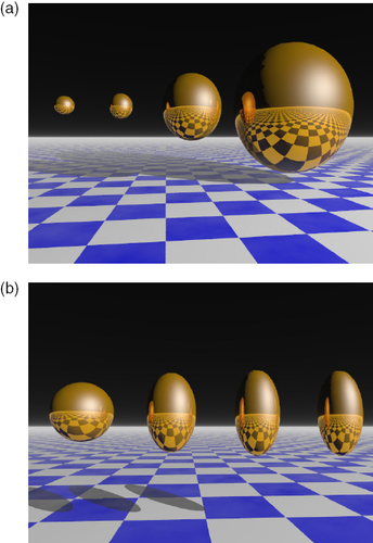
The effect of a magnetic field on Ostwald ripening was numerically investigated for several different physical conditions. In figure , several intermediate precipitate shapes are displayed as a function of time for two different estimated interface energies (0.1 and 0.01 J m−2). In both cases, there is evidence that the magnetic field causes anisotropic growth. For the higher interface energy, shape distortion occurs while there is a continuous growth in all directions. For the lower interface energy, the growth rate is lower and the shape evolves with growth at the magnetic poles and shrinkage on the equatorial belt.
Figure 1 Rendered view of the shape evolution during the growth of a ferromagnetic precipitate in a magnetic field. The physical conditions are as follows: roffset=1 μm, Initial shape is a sphere with 1015 vertices and radius r0=1 μm, μ0M=1 T, Bext=10 T, and is vertical in the images, μ C0 dt=10−3 (with oversampling down to 5×10− 5 for calculation of curvature effect). Images are shown every 33 steps of the calculations starting from the initial spherical shape. (a) γ=0.1 J m− 2 and (b) γ=0.01 J m− 2.
Ellipsoidal shape
In all simulations with the magnetic field applied along the z-axis, the coordinates of all vertices were plotted with z2 as a function of x2+y2 (where x and y are the two axes perpendicular to z). It was experimentally found that the relationship between z2 and x2+y2 coordinates was always linear, as shown in figure .
Figure 2 The shape of a growing precipitate under a magnetic field can always be fitted as an ellipsoid when starting from a spherical shape, as shown from the linear plot of z2 versus x2+y2. Here, the physical initial conditions are as follows: roffset=1 μm, B=6 T, μ0M=1 T, χat=5×10− 32, T=1200 K, γ=0.01 J m− 2, μ· C0 dt=10− 3 (with oversampling down to 5×10− 5 for calculations of curvature effect) 100×20 steps. Initial shape is a sphere with 1015 vertices and radius r0=1 μm.
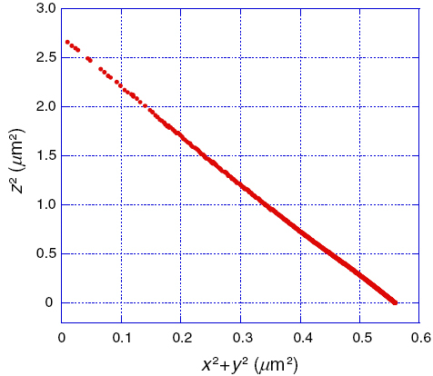
This suggests that in all 3D simulations starting from an initial spherical shape, the evolving shape can always be fitted using an ellipsoid. Hence, the long semi axis c and short semi axis a are sufficient to define the shape evolution of the growing precipitate.
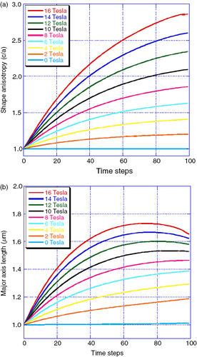
Field dependence
In figure , the shape anisotropy c/a and the long semi axis c are plotted as functions of the calculation time step. The experimental numerical results demonstrate that the effect of the magnetic field on shape anisotropy is not saturated in low fields as may be expected from the conventional effects of a torque or a demagnetizing field [Citation3]. The driving force for this effect is the gradient of the magnetic energy of the paramagnetic ions in the matrix, this gradient is in a first approximation proportional to the field gradient given by the ferromagnetic particle field multiplied by the magnetization of the ion, which is mainly proportional to the external field. For external fields above the local field Bsurf created by the particle, the total square field value B2=(B0+Bsurf)2 is almost equal to B02+B0Bsurf; as Bsurf does not depend on the external field B0 (once the ferromagnetic particle is saturated) and as B0 is uniform, the magnetic energy gradient is then proportional to B0 multiplied by the gradient of Bsurf. An almost linear dependence of the magnetic driving force on B0 (the external applied field) is thus expected once the particle magnetization is saturated.
Figure 3 Ellipsoid shape evolution during precipitate growth under strong external magnetic field. The initial physical parameters are as follows: roffset=1 μm, μ0M=1 T, χat=5×10− 32, T=1200 K, γ=0.01 J m− 2, μ·C0 dt=10− 3 (with oversampling down to 5×10− 5 for calculations of the curvature effect). 100 steps in calculation. Initial shape is a sphere with 1015 vertices and radius r0=1 μm, B=0-2-4-6-8-10-12-14-16 T (from lower to upper curves). (a) c/a (ellipsoid long axis/short axis) versus time and (b) c versus time.
Physical parameters governing the growth
In addition to the magnetic field intensity, the other parameters governing the growth are the ion atomic susceptibility χat, the temperature T, the interface energy γ and the initial supersaturation of the matrix Ci, which can also be expressed in terms of the offset radius roffset that a spherical particle has when in equilibrium with the matrix.
The ion atomic susceptibility χat is directly related to the magnetic force attracting the single ions around the magnetic poles of a growing precipitate. In the calculations of the interface growth (equation (10)), the magnetic driving force (χatB2) is proportional to χat. A linear effect, similar to the dependence on the external magnetic field intensity is then expected. | |||||
The temperature T plays a double role. Firstly, the particle must be ferromagnetic to induce strong local gradients: hence, the temperature should not exceed the curie point of the ferromagnetic phase. Secondly, the thermal activation energy kT always counterbalances the effects of both the magnetic field and the curvature as can be seen from equation (10). The driving forces for the growth itself and for the anisotropy of the growth are then both inversely proportional to the absolute temperature T. | |||||
As can be seen from figures (a) and (b), the interface energy γ plays a major role in the anisotropic growth of the precipitate. As expected from the physical mechanisms involved, the interface energy tends to produce spherical shapes whereas the local magnetic forces tend to produce elongated shapes. However, the effect of the magnetic field is not size dependent, since the local magnetic field depends on the geometry of the particle and not on its size. In contrast, the effect of the curvature varies inversely with the particle radius; for small sizes, the curvature effect should dominate, while for larger sizes, the magnetic field should control the growth. A secondary and less obvious effect can also be seen in figures (a) and (b) Starting from a particle in equilibrium with the matrix, a smaller interface energy leads to a greater effect of the magnetic forces: the particle elongates at the poles but also markedly shrinks on the equatorial plane. As a result, the particle volume growth (figure (b)) is much lower than that for the larger interface energy (figure (a)). | |||||
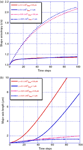
The initial supersaturation of the matrix CI (which can be expressed in terms of the equilibrium radius roffset) has a major effect on the particle growth. In a zero magnetic field, a spherical particle with a radius less than roffset will dissolve, whereas a particle larger than this threshold will grow. | |||||
The effect of matrix supersaturation on the particle growth has been calculated for two values of roffset, 100 or 90% of the initial particle size, and with γ (the interface energy) being equal to 0.1 or 0.01 J m−2. As shown on figure (a), the shape anisotropy is only slightly dependent on the matrix supersaturation. On the other hand, as can be seen in figure (b), the matrix supersaturation (or roffset) markedly affects the precipitate growth. As a first approximation, we conclude that the initial matrix supersaturation is mainly responsible for the average growth rate of the precipitate, while the magnetic field drives the anisotropy of the growth.
Figure 4 Evolution of precipitate growth under strong external magnetic field. The initial physical parameters are as follows: roffset=1 or 0.9 μm, μ0M=1 T, χat=5×10− 32, T=1200 K, γ=0.1 or 0.01 J m− 2, μ·C0 dt=10− 3 (with oversampling down to 5×10− 5 for calculations of curvature effect) 100 steps in calculation. Initial shape is a sphere with 1015 vertices and radius r0=1 μmB=10 T. (a) c/a (ellipsoid long axis/short axis) versus time and (b) c versus time.
Conclusion
A new mechanism of magnetic texturing during grain growth in the solid state at high temperatures was proposed. The local magnetic forces acting on single diffusing paramagnetic ions around a ferromagnetic precipitate induce preferential growth near the magnetic poles of the precipitate. Although usually neglected in the explanation of magnetic field effects, this magnetic interaction is demonstrated to control the anisotropic growth of an initially isotropic spherical precipitate.
It was experimentally shown that starting from an initial sphere, a precipitate growing under a strong magnetic field always evolves with an ellipsoid shape.
The main parameters governing the growth are the interface energy, the external field strength and the matrix supersaturation radius. The growth of the particle and the evolution of shape anisotropy are linked in a complex manner to these factors. Qualitatively, the magnetic field, which causes the particle to elongate, has the opposite effect to the surface energy, which tends to maintain a spherical shape. The matrix supersaturation plays a major role in the growth, but only slightly modifies the evolution of shape anisotropy.
More numerical experiments, together with other experimental observations of magnetic alloys are required to fully clarify the role of each factor. In addition, the model developed in this paper can be improved by taking into account the bulk diffusion in the matrix and the evolution of supersaturation with time.
References
- GaucherandFBeaugnonE2001 PhysicaB 294–295 96 http://dx.doi.org/10.1016/S0921-4526(00)00617-7
- GaucherandFBeaugnonE2004 PhysicaB 346–347262 http://dx.doi.org/10.1016/j.physb.2004.01.062
- BeaugnonEArrasE2006 J. Phys.: Conf. Series 51439 http://dx.doi.org/10.1088/1742-6596/51/1/101
- KittelC 1985Physique de l’Etat Solide, Dunod Université, ISBN 2-04-010611-1