Motorised digital levels: development and applications

Abstract

A low-cost motorisation of the Leica DNA03 digital level was designed to enable the automatic monitoring of deformations without compromising its manual use in levelling. The upgrade of the instrument and its electronic control system are described together with laboratory tests carried out to study the effects of ambient temperature on the level. A simple model for the correction of measurements as a function of the temperature is proposed. The detection of vertical movements with sub-millimetre accuracy was obtained in a simulated permanent monitoring system. The operational advantages of the instrument are shown in a field test. Despite the encouraging results, research is still needed to find a reliable model for the correction of the staff readings under changing temperature conditions.

Keywords:

• Digital level
• Monitoring
• Motorising levelling

Introduction

The monitoring of deformations of structures and infrastructures is increasingly carried out with integrated techniques in which the classic deformometers, such as inclinometers, extensometers or strain-gauges, are combined with automated surveying instruments. The latter can operate without human intervention, acquiring measurements and recording and transmitting them to a remote data processing centre where the coordinates of the monitoring points and their variations are determined in real-time. Examples of automated geodetic tools are robotic total stations and global navigation system satellite (GNSS) receivers.

Robotic total stations are modern total stations in which the rotational movements around both axes are performed by electric motors guided by automatic target recognition (ATR) systems, which enable the searching for and automatic pointing to prisms or reflecting targets. The recent development of instruments that use piezoelectric or electromagnetic motors has led to a substantial increase in the measuring speed, to the point that a truly continuous monitoring of a deformation process is possible 3.

In the case of GNSS, automatic monitoring systems are created with permanent stations. The type of receiver and modes of data acquisition and processing depend on the characteristics of the process to be monitored 5. In the control of rapid movements, for example, one can use network real-time kinematic networks (NRTK), in which the single monitoring point is a permanent GNSS station that receives a stream of data from the processing centre, which allows correction of the position of the monitored site in real-time. Technological innovation has recently led to the sale of instruments and specific software for the continuous control of structures, with an acquisition frequency of up to 20 Hz.

The versatility of both robotic total stations and GNSS receivers, used together or on their own, overcomes a great variety of problems encountered when monitoring structures or terrain. Nevertheless, there are many situations where the control of vertical movements alone is sufficient but requires sub-millimetre accuracy. The measurements of the settlements of building foundations, in tunnel construction, for grout injection or the structural testing of bridges are such cases. In these circumstances, the best measurement technique is digital levelling, in terms of operational simplicity and accuracy of the results 1, 8, 15.

Since the introduction of digital levels, the wish for an automation of the reading operation led to the creation of motion-controlled versions. Control systems based on motorised digital levels were realised for automatic measurements of vertical displacements.

Motorised version of the Leica NA 3000 and Zeiss DiNi 10 digital levels 10, 12, 13, 14, 17 were developed, in which a motion control motor points the instrument at the levelling bar code staffs and a second motor focusses the optics. The Zeiss DiNi 10T and 11T levels proved particularly suitable for monitoring thanks to their digital horizontal circle and the use of only 30-cm-long staff intervals for any distance up to 100 m. Another development 2 involved a rotating table powered by a stepper motor on which the levelling instrument is mounted. A second stepper motor operates the focussing mechanism. This device can be used for any type of digital level.

The measuring procedure is much the same for both solutions: a control computer is programmed to take sights and readings at any number of staff segments fixed to the structure points to be checked. The measuring system is initialised by manually entering the individual position of the staffs into the system. The azimuth positions and distances are then known. The computer will repeat the measuring cycle any number of times at time intervals determined by the user. The software takes the measurement values from each staff and compares them to a reference staff, calculating real-time absolute settlement. Moreover, the data processing software performs automatic calculations for the compensation of temperature influences, reducing the well-known problem of the temperature behaviour of the instruments. A study 10 pointed out the temperature effects on the Leica NA3000 level, with apparent changes in height reaching 2 mm at a distance between 10 and 20 m for 12°C of temperature variation. Another investigation 11 showed that the inclination of the line of sight of a Zeiss DiNi 11 varied from 0″ to 2·5″ from 20 to 50°C. Models for thermal correction, the use of two or three reference staffs and the analysis of time series are recommended by authors as a remedy. The accuracy of digital levels in the detection of vertical displacements suggested their use in 3D monitoring 9. For this purpose, Zeiss realised the DiNi 10T, called a ‘total level station’ 4. In this instrument, the absolute rotary encoder has a standard deviation of 2 mgon (≅7″).

Nevertheless, the many potential applications of motorised digital levels in civil engineering have not prompted the manufacturers to produce commercial instruments. The reason for the lack of success of such systems is probably their limited uses compared with the cost of the motorisation and control software. Therefore, we decided to investigate the possibility of realising a ‘low-cost kit’ for the upgrade of a precision digital level for use in automatic monitoring as well as in normal levelling. The instrument selected was a digital level Leica DNA 03, serial number 333561, made available by Leica Geosystems (standard deviation of height measurement per 1 km double-run after ISO 17123-2 0·3 mm km⁻¹ with invar staff; setting accuracy of the compensator 0·3″). A prototype meeting these requirements is presented in this paper. It features a simple electronic-mechanical upgrade of the level and a control software. The kit can be easily adapted to any DNA03 on the market or currently used by technicians. It is important to remark that the level may continue to be used for manual levelling because the slow motion and the focussing screws are accessible also with the motorisation device attached. The cost of the motorisation of an instrument is about 25% of the purchase price of the off-the-shelf instrument.

In this paper, the motorisation of the Leica DNA 03 and its control system are presented together with the results of laboratory tests carried out to study the effect of temperature variations on the instrument. Moreover, the use of the system in both fixed set-ups (for the monitoring of buildings subject to foundation settlements) and in temporary set-ups (for the testing of structures) is described.

Motorising of the digital level

The first prototype of a motorised DNA03 was built in 2005 (Fig. 1). For this model, stepper motors were used because they are easy to install, have great electrical and mechanical robustness and permit low speed of rotation and small angular rotations both clockwise and counter-clockwise. A console-joystick was used as the user interface.

Figure 1. Main components of the first prototype

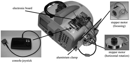
The prototype’s most important defect was the poor repeatability of the pointing to the levelling staffs. In fact, stepper motors were controlled in open-loop, estimating the position by counting the commutation steps applied to the motor phases. As a result, non-linear mechanical effects like Coulomb friction and backlash may affect the position estimation, because of a loss of steps during the counting of the phase commutations applied to stepper motors. We found that after a few hours, the level did not correctly point to the staffs anymore.

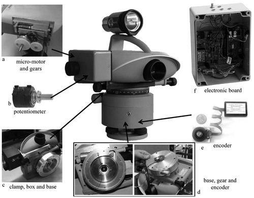
Therefore, a second system was developed where the stepper motors were replaced with an advanced mechanism based on coupled micro-motors and encoders in order to stabilise the rotation and improve the repeatability of the pointing to the staffs. In addition, a new external electronic board with firmware that commands the level and the movement system was built; finally, an easy-to-use graphic interface, installable on a PC, was developed to manage the level and the readings.

The robotisation ‘kit’ consists of (Fig. 2):

Figure 2. a micro-motor and gears used for automatic focussing; b potentiometer for the registration of the correct focussing position; c new plastic box containing the focussing motorisation, aluminium clamp built to fix the box to the instrument and upper part of the new aluminium base containing the motorisation used to rotate the level about the vertical axis; d micro-motor and gear mounted in the new base (left) and encoder mounted in the lower part of the new base (right); e encoder; f components of the external electronic board

Main components of the current implementation of the motorised Leica DNA 03 level

i.	electric motors: two electric micro-motors (DC-Micromotors and Faulhaber) to rotate the level about the vertical axis and to focus the levelling staffs are coupled with adaptors to reduce speed and increase torque
ii.	angular measurement: the micro-motor is coupled with an absolute encoder with resolution of 18 bits (Gurley Precision Instruments Inc., Mod.7700 and Virtual Absolute Encoder+VH Interpolating encoder) and is mounted in a new base under the instrument
iii.	focussing: the micro-motor is linked with a potentiometer to register the correct focussing position. Manual focussing is still possible thanks to an external screw
iv.	control system: a new electronic board to manage the level and the movement system was built. Its main component is a microprocessor whose serial ports are connected to the instrument by cable (via the RS232 standard port). In addition, an EEPROM memory allows the registration of settings related to the levelling staffs (angular position and focussing). All set-up operations and instructions, as well as the reception of the readings and the transfer of the data to the laptop/PC, are run by the related firmware
v.	connection with the laptop/PC: the connection between the electronic board and the laptop or the PC is realised by Bluetooth or by data transmission over the mobile phone network
vi.	user interface: a graphic interface developed in Visual C#, installable on a standard laptop/PC with the operating system Microsoft Windows XP or later, allows the remote control of the system, reception, registration and visualisation of the staff reading data directly on the computer screen by means of Bluetooth technology or data transmission over the mobile phone network [general packet radio service (GPRS)]
vii.	illumination: since the instrument takes measurements continuously, it is essential that it can operate when natural or artificial illumination of the staffs is lacking. Therefore, an illumination device based on LED technology was created, provided with dedicated circuits and powered directly by the external electronic board. Biconvex lenses concentrate the light emitted by a single LED so as to illuminate staffs as far as 50 m from the instrument.

The operation of the monitoring system requires a few simple steps. First, the level is set up on a tripod, a console or a concrete pillar and is protected against atmospheric influences. The levelling staffs or strips of coded ribbon are placed on one or more stable reference points and on the monitoring points. Then the user carries out the following operations:

i.	level the instrument using the three foot screws
ii.	switch on the instrument and the laptop/PC
iii.	switch on the external electronic board and start the program on the laptop/PC
iv.	connect the instrument and the laptop/PC via Bluetooth using the graphic interface
v.	manually point and focus to the first levelling staff
vi.	record these two settings using the program
vii.	repeat steps (v) and (vi) for the staffs on all reference and monitoring points (the levelling staffs are then read in the same sequence as they are registered)
viii.	set the stand-by time between one measurement cycle and the following (non-stop measures are also allowed) using the graphic interface
ix.	select the data transmission (Bluetooth or GPRS)
x.	save all the settings (they are automatically stored in the memory of the electronic board) and start the first automatic measuring cycle by pushing the START button in the graphic interface.

After these operations, the level automatically points to the staffs in sequence, applies the correct focussing screw setting, takes the readings and, when the cycle is complete, sends the values of the single readings, the time at the beginning of the cycle and the temperature of the instrument (recorded by the level’s internal thermometer) to the laptop/PC. When the procedure is complete, the level is automatically switched off. At the end of the selected stand-by time, the level is automatically switched on and begins the second cycle, and so on. It is possible to stop the instrument at any time and to reset all settings (if the cycle has already started, the instrument ends it, sends the data and then stops). After the set-up is completed, the PC can be switched off only if the data are transmitted using GPRS; otherwise, if a Bluetooth transmission is adopted, the PC must remain close to the instrument to receive and visualise the data in real-time.

Testing of the motorised level

First, the motorised level was tested to determine the accuracy and repeatability of the angular pointing and the motorised focussing. The system was highly reliable in focussing the staffs, while the angular pointing was governed by the resolution of the encoder and non-linear mechanical effects, like backlash and Coulomb friction. Because of these effects, the control loop can achieve only an actual pointing precision of 0·018° (corresponding to a pointing error of 6·28 mm at 20 m), even though the encoder resolution of 18 bits should theoretically allow a pointing error of <0·002°. As a consequence, a loss of the correct angular pointing to the invar levelling staff may occur for distances over 20 m. In these cases, wider coded staffs are recommended.

We then performed tests to:

i.	determine if the motorisation would compromise the instrument’s precision
ii.	study the effect of temperature variations on the readings
iii.	evaluate the instrument’s behaviour in simulated monitoring systems set-up indoors and out of doors.

It should be noted that all the tests have been made after the internal temperature of the instrument had stabilised.

Behaviour of the instrument in an environment with constant room temperature

Two tests were carried out in July 2009 in a tunnel usually used for nuclear physics experiments: one with the level ‘silent’ (motorisation deactivated), pointing to a single staff at a distance of 60 m from the level, the other with active motorisation, pointing to five staffs at distances of 5, 10, 20, 40 and 60 m (Fig. 3).

Figure 3. Layout of the tests in a constant environment (tunnel for nuclear physics experiments)

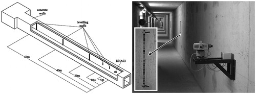
The first test lasted about 10 days. Using the purposely written control software, the instrument automatically repeated ∼1400 readings (one every 10 minutes) of an invar staff at a distance of 60 m (limit imposed by the length of the tunnel) and firmly attached to the reinforced concrete wall of the tunnel. Figure 4 illustrates the staff readings (below) and the temperature recorded simultaneously by the instrument’s thermometer (above).

Figure 4. Results of the first test at a constant temperature. The figure shows both the staff readings (left axis) and the temperatures (right axis)

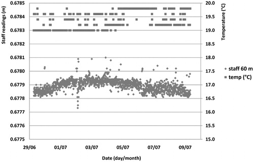
The staff readings have a standard deviation of 0·05 mm about the mean (better than the standard deviation due to the compensator sensitivity, 0·086 mm at 60 m) and a range of 0·37 mm. This first test showed that the modifications of the level did not alter the stability of its measurement system (with motorisation deactivated).

In the second test inside the tunnel, we activated the level’s motorisation, pointing to five invar staffs (always fixed to the tunnel walls) at 5, 10, 20, 40 and 60 m distance from the instrument (Fig. 3). This test lasted 8 days during which ∼2000 measurement cycles were performed (one cycle every 5–6 minutes). The measurements were essentially continuous, without interruptions between cycles. Figure 5 shows the readings of the different staffs and the temperature recorded by the level.

Figure 5. Second test in the tunnel performed in July 2009. a Trend of the temperatures and the staff readings at: b 5 m, c 10 m, d 20 m, e 40 m and f 60 m. For the staff readings, the vertical axis always presents a range of 1 mm in order to facilitate the comparison of the different measurements

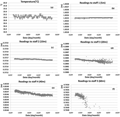
There is an increase in the dispersion of the readings as the distance increases (staff reading routine, atmospheric turbulence, etc.). In many cases, the instrument was not able to read the staff at 60 m because of the errors in pointing to the staff due to the limited resolution of the angular encoder used for the present implementation. To resolve this problem, it would have been necessary to use staffs or staff segments with a wider bar code, no longer on invar but on a less expensive material (aluminium, etc.), decreasing the overall precision of the test. In view of the metrological nature of these tests, we preferred to use only invar staffs. There is also a decreasing trend of the readings in Fig. 5, probably related to a small progressive decrease in temperature that occurred in the tunnel. For each staff, we calculated the range and standard deviation of the readings (Table 1). Figure 6 shows the linear increase in the standard deviation of the readings with increasing distance. The results of these tests demonstrate the performance of the motorised level in an ideal environment.

Figure 6. Graph of the standard deviation of the staffs readings shown in Table 1

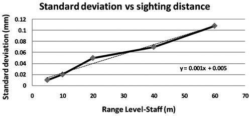
Table 1. Range and standard deviation σ of the readings for staffs at increasing distances

Distance/m	Range/mm	σ/mm	N readings
5	0·05	0·01	2083
10	0·10	0·02	2081
20	0·27	0·05	2080
40	0·31	0·07	2083
60	0·60	0·11	512

*N readings indicate the number of successful readings.

Behaviour of the instrument in an environment with regular temperature variation

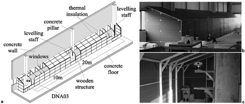
To study the effects of temperature variations on the digital level readings, we created an environment in which we could control the temperature at will. Inside an engineering laboratory, we constructed a tunnel ∼25 m long in a light material endowed with strong insulation properties (Fig. 7). The instrument was placed inside this environment on a steel shelf fixed to a reinforced concrete pillar. Two levelling staffs at 10 and 20 m from the level were fixed to other two reinforced concrete pillars. The environment was subjected to phases of heating and cooling lasting a few hours in order to simulate regular temperature variations, i.e. with constant speed. To do this, we used the heating/cooling system of the laboratory when possible; otherwise we switched on two additional electric radiators to get a fast increase in the temperature or we removed few thermal insulation panels when fast cooling was needed (all these test were performed in winter). In addition, several fans were set up to ensure a uniform temperature distribution and to reduce the horizontal and vertical thermal gradients to a minimum. The uniformity of the environmental temperature was checked with four probes 5 m apart from each other. In the numerous tests, the temperatures recorded by the level’s internal thermometer largely coincided with those recorded by the probes. Only in the situations of fast temperature variations did the level’s thermometer show a delay of a few minutes with respect to the probes. Nevertheless, we decided to use the datum provided by the level as the environmental temperature since it was always available in digital form together with the staff readings.

Figure 7. a 3D axonometric view; b external view of the ‘tunnel’; c internal view of the ‘tunnel’ with motorised level on a steel shelf fixed to a concrete pillar

‘Tunnel’ created for the controlled temperature tests

Hereafter, we illustrate the most important of the several dozen tests performed in order to demonstrate the instrument’s behaviour. In each test, the level automatically performed measurement cycles on both staffs at 10 and 20 m, with the time intervals between cycles varying from a few minutes to 30 minutes mainly in relation to the temperature variations. We only illustrated the trend of the staff readings at 20 m (the greater distance from the instrument) since it allows us to better demonstrate the effect of the ambient temperature.

It is possible to divide the tests into three classes based on the imposed temperature variations:

i.	class 1: slow temperature variation: regular variation with a speed of the temperature change lower than 2·0°C h−1 (positive or negative)
ii.	class 2: intermediate temperature variation: regular variation with a speed of the temperature change between 2·0 and 7·0°C h−1 (positive or negative)
iii.	class 3: rapid temperature variation: regular variation with a speed of the temperature change higher than 7·0°C h−1 (positive or negative).

The results of the first group of tests are illustrated in Figs. 8 and 9. Figure 8 describes a test lasting ∼4 h during which we reduced the temperature by 5·1°C, i.e. about −1·3°C h⁻¹. The staff readings at 20 m showed a decrease of −0·22±0·043 mm (the trend and standard deviation were obtained from a least squares linear regression line), corresponding to a downward change of the line of sight of about 2·29±0·45″ (0·45±0·09″ °C⁻¹).

Figure 8. Example of a test over 20 m belonging to the first class: slow and regular temperature decrease (less than −2°C h⁻¹); the figure shows both the temperature (right axis) and the staff readings (left axis) with the linear regression line

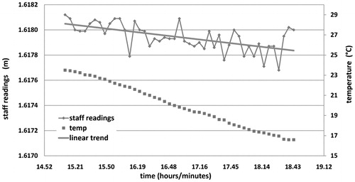
Figure 9. A second example over 20 m belonging to the first class of tests: slow and regular temperature increase (<2°C h⁻¹ in absolute value); the figure shows both the temperature (right axis) and the staff readings (left axis) with the linear regression line

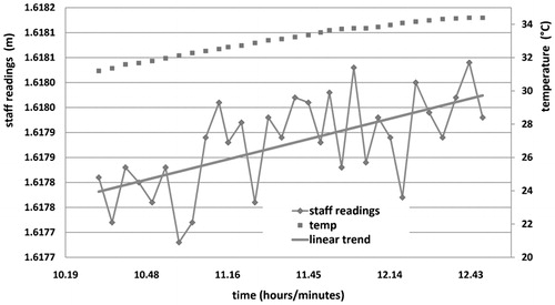
Figure 9 illustrates a test lasting around 2·25 h during which we imposed a temperature increase of +3·2°C (1·42°C h⁻¹). The staff readings at 20 m increased by +0·19±0·029 mm (on the basis of the least squares linear regression line), corresponding to an upward tilt of the line of sight of 1·98±0·30″ (0·58±0·09″ °C⁻¹).

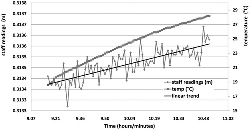
The second class of tests was characterised by an intermediate speed of temperature change (between 2 and 7°C h⁻¹, positive or negative). Figure 10 shows one of these tests: temperature increase of 9·6°C in 1·5 h (6·4°C h⁻¹). The result was an upward tilt of the line of sight of 1·98±0·17″ (0·21±0·018″ °C⁻¹) and an increase in the staff readings of 0·19±0·016 mm. A similar behaviour was recorded with a temperature decrease of intermediate speed. In this case (data not shown), there was a decrease in the staff readings of a magnitude (in absolute value) comparable to that in Fig. 10 (example: temperature decrease of −4·2°C h⁻¹, tilt of the line of sight of −1·50±0·12″ and decrease in the staff readings of −0·14±0·011 mm).

Figure 10. Example of a test over 20 m belonging to the second class: speed of (absolute) temperature change between 2 and 7°C h⁻¹; the figure shows both the temperature (right axis) and the staff readings (left axis) with the linear regression line

Third class of tests: rapid temperature variation. Figure 11 illustrates the results of a test with a temperature decrease of −12·7°C in 1 h and 10 min, i.e. with a speed of −10·9°C h⁻¹. The staff readings increased by +0·36±0·055 mm because of an upward tilt of the line of sight of 3·4±0·57″ (0·30±0·045″ °C⁻¹). Therefore, in this class, there was an inversion of sign between variation of temperature and variation of readings. A similar result (data not shown) occurred with a rapid increase in environmental temperature. Table 2 is a summary of the results obtained in the tests described thus far.

Figure 11. Example of a test over 20 m belonging to the third class: rapid temperature variation (>7°C h⁻¹ in absolute value); the figure shows both the temperature (right axis) and the staff readings (left axis) with the linear regression line

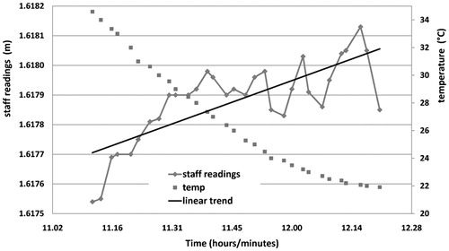
Table 2. Summary of the results of the described tests: class; duration of the test in hours; temperature difference between beginning and end of test; applied rates of temperature variation; variation of staff readings at 20 m, from linear regression line; rotation of the line of sight and rotation/temperature variation ratio

Test	Class (rate)	Test duration/h	ΔT/°C	Rate ΔT h^−1/°C h^−1	Tilt line of sight (20 m)/mm	Tilt line of sight/″	Tilt line of sight per °C/″ °C^−1
1	1° (ΔT<|2| °C h^−1)	4·00	−5·1	−1·30	−0·22±0·043	−2·29	−0·45
2	1° (ΔT<|2| °C h^−1)	2·25	+3·2	+1·42	+0·19±0·029	+1·87	+0·58
3	2° (ΔT = |2÷7| °C h^−1)	1·50	+9·6	+6·40	+0·19±0·016	+1·98	+0·21
4	3° (ΔT>|7| °C h^−1)	1·16	−12·7	−10·9	+0·36±0·055	+3·40	+0·30

All tests showed a clear correlation between the ambient temperature change and the staff readings. In the case of slow temperature variations (less than ±2°C h⁻¹), the tilt of the line of sight was ∼0·5″ °C⁻¹ and the sign of the temperature change was respected: an upward tilt corresponded to a positive temperature variation and vice versa. These results are valid for the tested digital level Leica DNA 03 Nr. 333561. The effects of the changes in ambient temperature on digital levels have been known for a long time. A study 7 pointed out a tilt of the line of sight of −0·52 and +0·37″ °C⁻¹ for the Zeiss DiNi 10 and a tilt of 0·33 and 0·34″ °C⁻¹ for the Leica NA 3003 (respectively in test of decrease and increase in the temperature), while another study 16 reported 0·5″ °C⁻¹ for the Sokkia SDL 30.

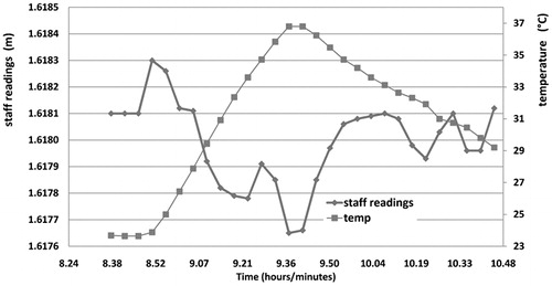
At faster temperature changes (2–7°C h⁻¹), the tilt of the line of sight decreased in value, albeit not in a linear manner (passing from ∼0·5 to ∼0·2″ °C⁻¹), but the sign of the temperature variation was still respected. For even faster temperature changes (>7°C h⁻¹ in absolute terms), the instrument showed an anomalous behaviour characterised by reversals of the sign (decreasing readings with strong temperature increases and vice versa). This type of test was repeated numerous times, also with positive and negative temperature variations in sequence, as exemplified by the test illustrated in Fig. 12: in a time interval of only ∼2 h, the temperature underwent an initial rapid increase of 13·2°C, followed by a decrease of −7·6°C. The staff readings showed an initial decrease until a maximum of 0·45 mm (at a distance of 20 m) and a subsequent increase to values near those at the beginning of the test, confirming the inversion of sign between temperature variation and staff reading variation. A similar behaviour was reported for a Leica NA3003 in the first 30 min of a test 7. A sign reversal after an overcorrection caused by a fast temperature change is reported in 6 for a Zeiss DiNi 10.

Figure 12. Trend of the staff readings at 20 m in relation to two consecutive rapid temperature changes of opposite sign (>7°C h⁻¹); the figure shows both the temperature (right axis) and the staff readings (left axis)

In conclusion, for slow environmental temperature variations (below 2°C h⁻¹) typical of indoor environments, it is possible to correct the staff readings in real-time. In this case, a simple linear model could be used(1) where dL(t) is the staff reading correction at time t, T is the temperature at time t, T₀ is the temperature at start-time t₀, D is the distance from the level to the staff and k is the tilt of the line of sight, taken as 0·5″ °C⁻¹ for the particular instrument tested (see Table 2). This model can be applied, for instance, in the case of permanent monitoring systems like those illustrated in the next section. The k value has to be determined for each individual digital level. For more rapid temperature variations, we were unable to identify a mathematical model for the correction of the staff readings.

Simulation of a permanent monitoring system

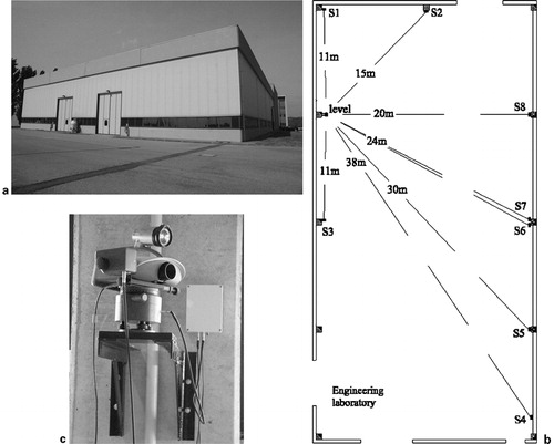
To evaluate the instrument’s response in a permanent monitoring system, we conducted tests of medium–long duration inside an industrial engineering laboratory (Fig. 13). The motorised level was mounted on a shelf rigidly fixed to a reinforced concrete pillar about 3 m above the floor in a position not subjected to direct sunlight. Eight levelling staffs were used at distances varying from 11 to 38 m. They were invar staff segments fixed to eight reinforced concrete pillars. Since the structure was stable, the monitoring points were not subject to any type of settlement. In any case, points S1 and S3 (Fig. 13) were considered reference points during the tests. It must be remarked that the positioning of the reference points was not optimal. If temperature effects are expected and need to be corrected for, the reference points should be as far away from the instrument as possible. The tests lasted from a few days to several tens of days during which the instrument automatically performed a measurement cycle every 30 min.

Figure 13. a permanent monitoring of an industrial building, b positions of the monitoring and reference points and of the level and c detail of the set-up of the level mounted on a bracket

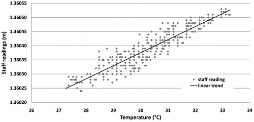
In one of the most significant tests, lasting around 8 days, there was a mean temperature increase of +3·9°C and a mean increase in the staff readings at 20 m (point S8) of +0·23±0·005 mm, corresponding to a tilt of the line of sight of +2·39±0·052″ (0·61±0·013″ °C⁻¹). The trend of the environmental temperature recorded by the level’s thermometer and the trend of the staff readings are shown in Fig. 14. Again, in this case, there is a clear correlation between the staff readings and the temperature, also shown by a coefficient of correlation between the two data series of 0·932 and by the scatter plot shown in Fig. 15. It is easy to identify a periodic signal with a period of around 24 h (diurnal temperature variations) in both the staff readings and the ambient temperatures. However, the speed of the temperature variation is always lower than 2°C h⁻¹.

Figure 14. Correlation between staff readings and temperature for an 8-day test. Staff readings at 20 m (below, left axis) and temperature values (above, right axis)

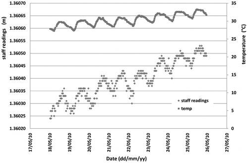
Figure 15. Scatter plot of staff readings versus temperature for a staff at 20 m (same data as in Fig. 14)

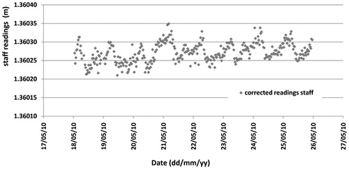
The readings of each staff were corrected according to the correction model described in equation (1) based on the difference between the ambient temperature of each reading and the temperature at the beginning of the test. Figure 16 reports the corrected values for a staff at 20 m: these data have a standard deviation of 0·036 mm and a range of 0·17 mm. In a permanent monitoring system, this correction model could easily be applied in real-time.

Figure 16. Corrected values of staff readings at 20 m. All corrected measurements (100%) are in a range of 0·2 mm

If the variation of the staff readings is highly correlated with that of the temperatures, it may be possible to correct the staff readings a posteriori using various correction models parameterised on the measurements themselves. For instance, a simple model could involve the sum of a trend (linear or not) with one or more periodic signals of fixed frequency λ_j, of the type(2) where L(t) is the staff reading at time t, a_i is unknown parameter of the trend, b_j and c_j are unknown parameters of the periodic signals of fixed frequencies l₁, …, l_k and Y(t) is a random noise component.

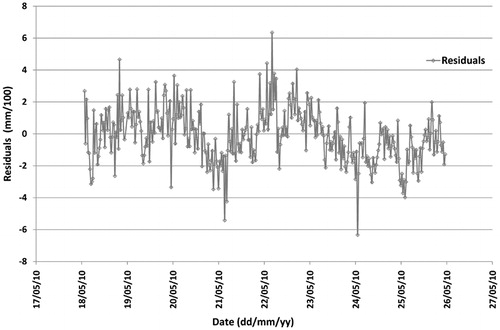
For the staff measurements at 20 m reported in Fig. 14, the trends of the ambient temperature and of the staff readings can be described by a simple linear trend and a single periodic signal, with the period determined on the basis of the periodogram of the temperature time series (in the example, there is a period of 44 measurements per day: a little more than 30 min between one measurement and the next). In this way, equation (2) can be simplified to(3) Based on the data shown in Fig. 14, we determined the parameters a, a₁, b and c with a least squares regression estimation and obtained the trend reported in Fig. 17 superimposed on the staff readings at 20 m. Correcting the staff readings by values computed with equation (3), we obtained the residuals shown in Fig. 18; these residuals represent a standard deviation of 0·016 mm and have a range of 0·12 mm. They are very similar to those obtained from the application of the correction model in real-time (Fig. 16).

Figure 17. Staff readings at 20 m are superimposed by a linear trend and a single periodic signal, whose coefficients were determined by least squares estimation

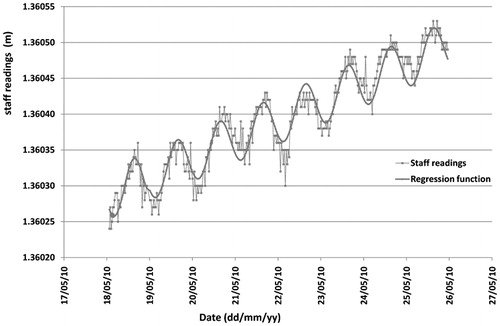
Figure 18. Residuals about the trend function shown in Fig. 17

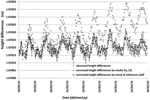
In a permanent monitoring system, one or more stable reference points are used and the variations of the height differences measured to the monitoring points are analysed with respect to the reference points. For monitoring points at the same distance from the level as the reference points, the effect of temperature variations on the level is directly cancelled in the calculation of the height difference. For monitoring points at different distances, such temperature effects may be reduced with a simple propagation of the linear trend calculated from the readings of the reference staff multiplied by the distance of the monitoring points. As alternative, the proposed correction model of equation (3) can be applied for the monitoring points. Figure 19 (diamond symbols) shows the trend of the height differences observed between a monitoring point at 20 m from the level and a reference point at 11 m. The sum of a linear trend and a daily periodic signal are also evident for the height difference. The measurements of this height difference have a standard deviation of 0·085 mm and a range of 0·39 mm. Applying the correction model of equation (3), we obtain a standard deviation of 0·036 mm and a range of 0·20 mm for the corrected height differences (Fig. 19, line with squares). Very similar results were obtained by applying a correction using the trend of the readings of the reference staff (at a distance of 11 m) multiplied for the ratio 20∶11 (distance to monitoring point/distance to reference point) (Fig. 19, line with triangles).

Figure 19. Observed height differences between a monitoring point at 20 m from the level and a reference point at 11 m from the level (points with diamond symbol); the same height differences corrected by equation (3) (line with squares) and height differences corrected by the trend of reference staff (11 m distance) multipled for a coefficient 20∶11 (line with triangles)

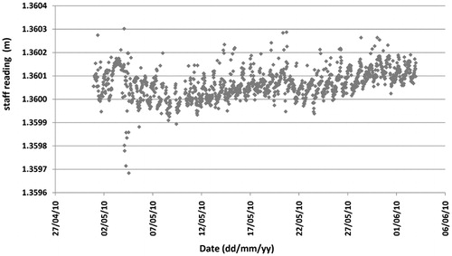
The monitoring was extended for a further 35 days in the same operational conditions. Figure 20 shows the trend of the staff readings at 20 m from the level and of the temperature. There are two episodes with temperature variations greater than 2°C h⁻¹ but lower than 7°C h⁻¹. Therefore, the previously described real-time correction model of equation (1), using k = 0·5″ °C⁻¹ for the tested instrument could be applied in this case; the corrected readings (Fig. 21) exhibit a standard deviation of 0·06 mm and a range of 0·62 mm. More than 97% of the corrected measurements are in a range of 0·3 mm.

Figure 20. Variation of staff readings over 20 m and temperature in a 35-day test. Staff readings at 20 m (below, left axis) and temperatures (above, right axis). There are two distinct jumps in the ambient temperature (4 May 2010 and 20 May 2010) causing jumps in the staff readings

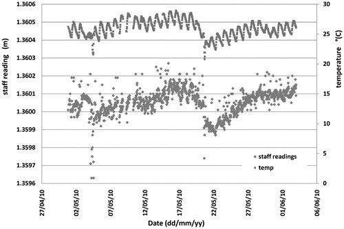
Figure 21. Corrected values of the staff readings of Fig. 20 using the real-time correction model of equation (1) with k = 0·5″ °C⁻¹ as determined for the tested instrument

Field test of a temporary monitoring system

The test of a structure, for instance a bridge or a floor, normally lasts a few hours, but can take several days for large structures with numerous load conditions. In these cases, it is not necessary to establish permanent benchmarks, and a temporary monitoring system is of advantage. It is set up at the beginning of the operation and removed at the end of the intervention.

The motorised level was tested for the structural monitoring of a bridge. This case-study concerns a reinforced concrete bridge with a depressed arch beam (width of the beam 10·55 m, and distance between the two supports 31 m). In this test, the monitoring points were created with coded levelling staffs attached to telescopic poles supported by a base with fixing bolts (Fig. 22). Since the test required many monitoring points, we opted for less expensive aluminium staffs, but corrected for the thermal expansion of the material (24 ppm °C⁻¹).

Figure 22. a the bridge, b the monitoring points (S1 to S5, at distances from the instrument between 6 and 34·5 m) and the trucks used to load the bridge, c layout of the monitoring system (including the single reference point, at a distance of 6 m from instrument) and d a detail of the coded staffs

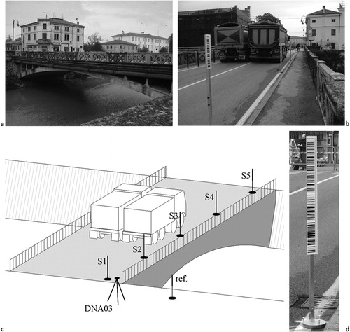
The levelling staffs were positioned in a single line, as it was impossible to monitor both sides of the bridge due to the trucks’ position during the full load test. Figure 23 depicts the results of one of the load tests carried out on the bridge; it illustrates the behaviour of the structure. As the temperatures did not affect the results of the test, we did not apply the real-time temperature correction. Corrections of few hundredths of millimetres were insignificant considering the maximum deformation under full load condition of 1·5 mm. To check the results obtained with the motorised digital level, we also performed manual levelling for each load condition: the differences between the two techniques did not exceed 0·3 mm.

Figure 23. Vertical displacements of the monitoring points S1 to S5 detected by the motorised DNA03 in relation to the load conditions. All displacements were obtained as difference between the reading to the reference staff (repeated for every cycle) and the reading to the single monitoring point

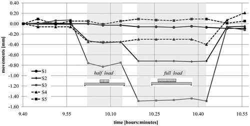
This test demonstrates the operational advantage of the motorised instrument. It was conducted by a single operator, with a marked saving in personnel costs. The real-time application of the model (equation (1)) for the correction of the readings for the temperature effects was not required on this occasion.

Conclusions

The motorisation of digital levels by users started several years ago. However, despite some interesting applications for the monitoring of vertical movements, motorised levels have not been commercially successful. This is probably due to the high cost of motorisation and their limited uses compared with robotic total stations. Therefore, we designed and built a prototype of a low-cost kit for the motorisation of the Leica DNA03 digital level for use in automatic monitoring as well as in manual levelling. The system consists in a simple electronic-mechanical upgrade of the level and a control software, running on a personal computer with operating systems Microsoft Windows XP or later.

The innovative character of the new motorisation lies in having developed a ‘kit’ that can be produced on an industrial scale at low cost, modifies as little as possible the design of the original instrument and also allows the use of the instrument in manual mode. Our prototype does not yet fully comply with these requirements. It is possible to further reduce the size of the motorisation, increase the speed of rotation and increase the angular resolution of the encoder in order to have sighting distances up to 60 m.

Under conditions of constant temperature, the instrument showed a good stability of the staff readings. Significant variations were detected when the ambient temperature changed. At temperature changes of less than ±2°C h⁻¹, the slope of the line of sight increased or decreased by 0·5″ °C⁻¹ for the specific instrument tested. As a consequence, a simple linear model can be adopted to correct the readings if the staffs are placed at different distances. Therefore, the instrument is suitable for indoor monitoring. For long-term monitoring, a model is suggested that also takes into account the diurnal trend of the readings. Unfortunately, we were not able to find a reliable model to correct the staff readings when the ambient temperature varies faster or when the trend of the temperature changes from increase to decrease and vice versa.

For this reason, a monitoring network should be designed with multiple reference points at appropriate distances from the level in order to correct measurements in real-time. If this is not possible, a model of correction of the readings can be used; this model has to be defined for the specific instrument as the result of suitable calibration, provided that the temperature variation is not too rapid.

The system was tested for short- and long-term monitoring. The thermal effect on other prototypes remains to be checked in order to detect inconsistencies in the behaviour between one instrument and another. For outdoor applications of the motorised level, it is important to continue the research into a model to correct the staff readings when the ambient temperature changes quickly. It will be interesting to study the simultaneous use of multiple instruments, offering the possibility to adjust observations in situations in which high accuracy is required. Finally, we hope that our low-cost adaptation of commercially available instruments will be an incentive for professionals to use motorised digital levels.

The authors thank Engineers Alessandro Zerbetto and Antonio Gonelli for their valuable assistance during the numerous tests and Engineer Nicola Preda for his contribution to the realisation of the control software for the motorised level. The authors wish to acknowledge constructive comments and suggestions provided by the anonymous reviewers.

References

- Albattah M., 2003. Landslide Monitoring Using Precise Levelling Observations. Survey Review, 37(288): 127–136.
- Beer C, Stoyan H. Motorised Digital Levelling Instrument – Automatic Precision Levelling with online Visualisation. http://www.angerer-cps.com (accessed 15 October 2012).
- Berberan A, Machado M, Batista S., 2007. Automatic Multi Total Station Monitoring of a Tunnel. Survey Review, 39(305): 203–211.
- Feist W, Gimm A, Marold T, Rosenkranz H., 1996. DiNi 10 T – The First Digital Total Level Station. Translation from Vermessungswesen und Raumordnung, 58(1): 1–7. Dümmler Verlag, Bonn. www.survey-solutions-scotland.co.uk/survey_ftp/Whites%20papers/Precision%20Levels%20White%20Papers/DiNi%2010T.PDF.
- Gokalp E, Tasci L., 2009. Deformation Monitoring by GPS at Embankment Dams and Deformation Analysis. Survey Review, 41(311): 86–102.
- Heister H., 2002. Zur Kalibrierung von digitalen Nivellier-Systemen (On the Calibration of Digital Levelling Systems). Allgemeine Vermessungs-Nachrichten (AVN), 109(11–12): 380–385 (in German).
- Helmstädter S, Meier-Hirmer B., 1997. Laboruntersuchungen zur Leistungsfähigkeit der Präzisionsdigitalnivelliere Wild NA3003 und ZEISS DiNi10 (Laboratory Tests on the Performance of Precision Digital Levels Wild NA3003 und ZEISS DiNi10). Vermessungswesen und Raumordung, 59(5+6): 296–304 (in German).
- Ingensand H., 1999. The Evolution of Digital Levelling Techniques – Limitation and New Solution. Paper to Jubilee Seminar: Geodesy Surveying in the Future, The Importance of Heights, 15–17 March 1999, Gävle, Sweden. http://www.fig.net/commission5/reports/gavle/ingensand.pdf.
- Ingensand H, Meissl A., 1995. Digital Levels on the Way to 3-D Measurement. In A. Grün and H. Kahmen, eds. Optical 3-D Measurement Techniques III, Wichmann Verlag, Heidelberg: 139–148.
- Keppler A, Meissl A, Naterop D., 1996. Automatische Bauwerksüberwachung mit motorisierten Digitalnivellieren. In: Brandstätter/Brunner/Schelling, eds. Ingenieurvermessung 96 (Beiträge zum 12. Int. Kurs für Ingenieurvermessung, Graz, 9–14 Sep 1996), Dümmler Verlag, Bonn: Vol. 1, A9/1–A9/10 (in German). http://www.solexperts.com/index.php?option = com_content&view = article&id = 246&Itemid = 48〈 = en.
- Menzel M., 1999. The Development of Levels during the Past 25 Years, with Special Emphasis on the NI002 Optical Level and the DiNi 11 Digital Level. ftp.ngs.noaa.gov/pub/corbin/precise-leveling-workshop/Equipment/Trimble_Zeiss/DiNi 11_and_Ni002_whitepaper.pdf.
- Naterop D., 1998. Automated Monitoring for Geotechnical Engineering Projects. Development of Geotechnical Tests. Chinese Association of Geotechnical Investigation, Seminar Beijing 1998. http://www.solexperts.com/index.php?option = com_content&view = article&id = 246&Itemid = 48〈 = en.
- Naterop D, Keppler A., 1998. Der Eisatz von Automatisierten Geodãtischen Messinstrumenten in der Geotechnik. Beispiele aus der Praxis, Messen in der Geotechnik, Braunschweig (in German). http://www.solexperts.com/index.php?option = com_content&view = article&id = 246&Itemid = 48〈 = en.
- Naterop D, Yeatman R., 1995. Automatic Measuring System for Permanent Monitoring: Solexperts Geomonitor. Proceedings of the 4th International Symposium on FMGH 95: Field Measurements in Geomechanics. SGEditoriali, Bergamo: 417–424. http://www.solexperts.com/index.php?option = com_content&view = article&id = 246&Itemid = 48〈 = en.
- Rekus D, Aksamitauskas VC, Giniotis V., 2008. Application of Digital Automatic Levels and Impact of Their Accuracy on Construction Measurements. Proceedings of 25th International Symposium on Automation and Robotics in Costruction, Institute of Internet and Intelligent Technologies, Vilnius: 625–631. http://www.isarc2008.vgtu.lt/
- Staiger R., 2002. Instrumentenuntersuchung des Digitalnivelliers SDL 30 von Sokkia (Instrument Testing of the Digital Level SDL30 from Sokkia). Allgemeine Vermessungs-Nachrichten (AVN), 109(11–12): 386–391 (in German).
- Thut A, Raz U, Naterop D, Becker H-J., 2002. Monitoring during Construction in Urban Areas. Proceeding of 2nd International Conference on Soil Structure Interaction in Urban Civil Engineering, ETH Zurich, Zurich: 489–496. http://www.solexperts.com/index.php?option = com_content&view = article&id = 246&Itemid = 48〈 = en.