Extendable linearised adjustment model for deformation analysis

Abstract

This paper gives a linearised adjustment model for the affine, similarity and congruence transformations in 3D that is easily extendable with other parameters to describe deformations. The model considers all coordinates stochastic. Full positive semi-definite covariance matrices and correlation between epochs can be handled. The determination of transformation parameters between two or more coordinate sets, determined by geodetic monitoring measurements, can be handled as a least squares adjustment problem. It can be solved without linearisation of the functional model, if it concerns an affine, similarity or congruence transformation in one-, two- or three-dimensional space. If the functional model describes more than such a transformation, it is hardly ever possible to find a direct solution for the transformation parameters. Linearisation of the functional model and applying least squares formulas is then an appropriate mode of working. The adjustment model is given as a model of observation equations with constraints on the parameters. The starting point is the affine transformation, whose parameters are constrained to get the parameters of the similarity or congruence transformation. In this way the use of Euler angles is avoided. Because the model is linearised, iteration is necessary to get the final solution. In each iteration step approximate coordinates are necessary that fulfil the constraints. For the affine transformation it is easy to get approximate coordinates. For the similarity and congruence transformation the approximate coordinates have to comply to constraints. To achieve this, use is made of the singular value decomposition of the rotation matrix. To show the effectiveness of the proposed adjustment model total station measurements in two epochs of monitored buildings are analysed. Coordinate sets with full, rank deficient covariance matrices are determined from the measurements and adjusted with the proposed model. Testing the adjustment for deformations results in detection of the simulated deformations.

Keywords:

• Deformation analysis
• Observation equations with constraints
• Rank deficient covariance matrix
• Affine
• Similarity and congruence transformation

Introduction

Geodetic deformation analysis is about analysing the geometric changes of objects on, above or under the earth’s surface or changes of this surface itself. The objects are generally discretised by points, whose coordinates are registered at two or more epochs.

Affine, similarity and congruence transformations play an important role in geodetic deformation analyses, mainly for two reasons. First objects may undergo deformations that are well described by such transformations. This is the case, if the deformations comprise translations, rotations, shears and changes of size. The second reason is that objects are often described with geodetically determined coordinates that are defined by geodetic datums. To transform coordinates to a common datum, transformations are necessary. The three mentioned transformation types are often adequate for this purpose.

Deformations of objects may comprise much more complicated patterns than can be described by congruence, similarity or affine transformations. Therefore extended functional models have to be built to describe the relations between coordinate sets of two or more epochs of geodetic measurements. These extended models can often be described as extensions to the congruence, similarity or affine transformation or to combinations thereof. If necessary the models are complemented by covariance functions (collocation) or variograms (kriging) to capture the systematic effects that are not described by the functional model.

Problem definition

The problem addressed in this paper is the problem of finding the relation between two coordinate sets in 3D, describing each object by means of the same points but at different moments in time. This relation describes the deformation that the object is subject to and a possible difference in geodetic datum. The coordinate sets are supposed to be Cartesian with full covariance matrices, reflecting the precision by which the coordinates have been acquired. Testing the correctness of the deformation model should be possible. If it is not correct, it should be possible to find least squares estimates of the deformations. These estimates can be used to extend the adjustment model.

Approach to solution

The problem is addressed by first finding the optimal affine transformation, or its special cases: the similarity and congruence transformation. Subsequently the transformation model is extended by additional parameters to find the best fitting solution.

The affine transformation in 3D involves a rotation. This rotation is often described by Euler angles. They have, however, the disadvantage that gimbal lock may occur, i.e. the impossibility to determine the three Euler angles, if a specific one of them is 0 or 90°. Which angle gives this problem and at what value, depends on the sequence in which Euler angles are applied to perform a rotation. If the problematic angle is close to the dangerous value, this may still cause problems to determine the other angles with sufficient precision. Therefore finding the deformation should avoid the use of Euler angles, because angles of 0 and 90° can occur in deformation problems.

The approach to solve the posed problem is setting up an adjustment model and solving the parameters of this model by means of the method of least squares. It is an adjustment model, because there are in general more coordinate differences than transformation parameters to be estimated.

The adjustment model describes a null hypothesis, in which it is supposed that no deformation occurred. It should be possible to extend the model with extra parameters to formulate alternative hypotheses, which describe possible deformations, and to test them against the null hypothesis. A linearised adjustment model makes it relatively easy to formulate many types of hypotheses. Linearisation of the model makes it easy as well to take account of full covariance matrices of coordinate sets. Such full covariance matrices are to be expected when the coordinate sets are the result of the adjustment of geodetic measurements (terrestrial, airborne or satellite).

Overview

The setup of this paper is as follows.

First the general adjustment model for a transformation is given. Determining the transformation parameters between two or more coordinate sets is a problem that can be solved without linearisation of the functional model, if the transformation is one-, two- or three-dimensional and an affine, similarity or congruence transformation. Direct solutions to the general adjustment model are referenced.

The paper continues with the linearised adjustment model. If the deformations are more than just an affine, similarity or congruence transformation, it is hardly ever possible to find a direct solution for the transformation parameters. Linearisation of the functional model and solving the linearised model is necessary in that case. The linearised adjustment model is given as a model of observation equations with constraints on the parameters. The starting point is the affine transformation, whose parameters are constrained to get the parameters of the similarity or congruence transformation. In this way the use of Euler angles is avoided.

The least squares solution of a linearised adjustment model is reviewed. It is shown how to handle a singular cofactor matrix. Methods to solve an adjustment problem with constraints are given.

Then the model for the affine transformation is elaborated upon, followed by the congruence transformation. A linearised adjustment model needs approximate values for the unknown parameters. Their determination and the iteration to arrive at the final solution are treated. In each iteration step approximate parameters are necessary that fulfil the constraints. For the affine transformation it is easy to get approximate coordinates. To make subsequently the approximate coordinates comply to the constraints, use is made of the singular value decomposition of the rotation matrix.

Finally the similarity transformation is treated and an experimental validation is given.

Recent literature mentions total least squares as a method to find a least squares solution for transformation problems, where all coordinates are considered stochastic (Fang, 2011; Snow, 2012). In this paper it is shown that it is very well possible to construct an adjustment model, where all coordinates are considered stochastic and the coefficient matrix does not contain stochastic elements. This makes application of the total least squares method unnecessary. Since standard method of least squares is, its extensive body of knowledge can be used.

General adjustment model for transformation

A general adjustment model for solving the transformation parameters between two sets of coordinates is treated in this section.

Let a point field be described by a set of Cartesian coordinates in reference system r_a, taken together in a vector a , and by another set of Cartesian coordinates in reference system r_b, taken together in a vector b . The vector names are underlined to indicate that they are random variables. It is supposed that vector a differs from vector b because of a deformation, a difference in geodetic datum and of stochastic noise in both vectors. Let the vector c contain the mathematical expectations of a , i.e. (1) where E{ } indicates the mathematical expectation.

Let a transformation, represented by the vector function t, transform the vector b into the vector a by means of transformation parameters, taken together in vector f. The transformation is supposed to describe the deformation and the difference in geodetic datum. The mathematical expectation of a and of the transformed vector b should then be equal (2)

The transformation t is non-linear in the elements of vector b and of vector f for the affine, congruence and similarity transformation. If, however, vector b is considered non-random, i.e. a constant vector, transformation t is linear for the affine transformation. Its direct least squares solution is given in section ‘Step 1: affine transformation done simply’.

For the general case transformation t is non-linear, which means that a solution can be found by a direct solution, treated in the next section, or by solving iteratively a linearised model, treated subsequently. This paper proposes a solution with a linearised model, which is elaborated upon in the section ‘Linearised adjustment model’.

Direct solutions

A direct solution of the transformation parameters in (2) is, as mentioned above, straightforward in the case of an affine transformation if b is considered a constant vector. The stochastic behaviour of b cannot be taken account of, unless it is possible to have it included in the stochastic behaviour of vector a .

In the case of a congruence transformation the transformation consists of a rotation around a certain axis and a translation in a certain direction. It can be considered a special case of the similarity transformation, treated subsequently.

The similarity transformation in 3D consists of a rotation around a certain axis, a translation in a certain direction and a change of scale. It is also called a seven-parameter transformation or a Helmert transformation (Awange et al., 2004; Krarup, 2006).

Much literature is devoted to finding direct solutions for the parameters of these transformations, where finding the three rotation parameters is most difficult.

Menno Tienstra writes (Tienstra, 1969) that the first method published was by Thompson (1959) and that Schut (1960/61) gave a more elegant derivation of the same method. Tienstra himself gives a different method (Tienstra, 1969). At least eight solutions of more recent date (from 1981 up to 2006) can be found in literature. They are the solutions of Hanson and Norris (1981), Bakker et al. (1989, p.55), Awange et al. (2004), Teunissen (1985, p.148), Arun et al. (1987), Hinsken (1987), Horn et al. (1988), and Krarup (2006).

Of the first three solutions a short description is given to illustrate the different approaches that are possible.

Hanson and Norris consider in their paper (Hanson and Norris, 1981) the estimation of the transformation parameters of the congruence and similarity transformations. Their application is quality control of manufactured parts, where points on parts are matched with points on a drawing. They prove that the least squares estimation of the rotation can be performed independently from the translation, if the elements of a and b are mutually stochastically independent and the x, y and z-coordinate of each point i have the same weight γ_i. A procedure is given to compute the direct least squares estimates of the rotation parameters by means of singular value decomposition of a matrix that is computed from the elements of a and b . Also a procedure is given to compute the direct least squares estimate of the change of scale of the similarity transformation. The direct least squares estimate of the translation is the difference between the centres of gravity of a and the rotated and scaled b .

Bakker et al. (1989) consider the points of a and b as a distribution of mass points with unit mass. They compute for both a and b the centre of mass, the set of body-axes, the mean radius of gyration and the inertia tensor. After translating to the centre of mass, rotating with the inertia tensor and scaling both a and b , the transformed vectors are equated and a formula for the transformation parameters derived. The stochastic characteristics of a and b are not taken into account, although it is mentioned by Bakker et al. (1989) that an adjustment is easy, especially if the coordinates have rotationally symmetric variances.

Awange et al. (2004) give a procedure to compute the least squares estimates of the parameters of the similarity transformation (seven-parameter transformation), based on finding the roots of univariate polynomials using a Groebner basis.

Solutions by linearisation

The transformation parameters in (2) can be solved by linearising the equation and using the standard least squares algorithm. The advantage of this approach is the possibility of solving adjustment models, for which direct solutions are not known. The disadvantages are the need to have approximate values for all unknown parameters and the need to iterate the computation with the risk of divergence, if the approximate values are not chosen well.

The linearisation of the affine transformation is simplest and is given first. For the linearisation of the congruence and similarity transformation, the rotation has to be parameterised. This is generally done, see e.g. Hofmann-Wellenhof et al. (2001, p. 294), by using three angles that describe the rotation around three coordinate axes, the so called Euler angles. As described in the introduction, the use of Euler angles may result in gimbal lock. This problem occurs for example for the rotation parameterisation of Hofmann-Wellenhof et al. (2001, p. 294), if the second rotation angle α₂ is a right angle (α₂ = 100 gon), which yields the rotation matrix R (3)

Only the sum (α₁ +α₃) appears in the matrix, and angle α₁ nor angle α₃ can be determined separately, although the rotation matrix itself is well defined. This is called ‘gimbal lock’ after the equivalent problem in mechanical engineering, when two of three gimbals become parallel to each other and one rotation possibility is lost. An additional disadvantage of Euler angles is that approximate values for them have to be determined in some way. In this paper a different approach is chosen, where the rotations are not parameterised by three angles, but by the nine elements of the rotation matrix. By imposing six constraints on the nine elements, the matrix is forced to describe only rotations.

The use of the direct solutions of the previous section has the advantage that no approximate values and no iteration are needed. The advantage of a linearised adjustment model, however, is that extending the model with other parameters is easy. There are two reasons why the model should be extended:

(i)	errors may be present in the coordinates, caused by errors in the measurements that were used to compute the coordinates, or caused by e.g. identification errors. To test for these errors the model is extended by parameters, describing these errors. The extended model is tested as an alternative hypothesis against the null hypothesis of no errors (Teunissen, 2006, p.78).
(ii)	the description by means of 6, 7 or 12 parameters of one congruence, similarity or affine transformation may be not adequate. Maybe not one but more such transformations are needed, for example each describing a subset of points. Or more complex transformations with more or other parameters are needed.

Extending or changing the model is easier for a linearised model than for a non-linear one.

Linearised adjustment model

Linearisation of general model

To solve the problem of finding the transformation parameters, a system of observation equations is set up. Constraints are added to this system. This constrained system is solved by means of the method of least squares. As the equations of this system are not linear, they are linearised.

First the system is given for an affine transformation. The affine parameters can be obtained without the addition of constraints. Then the system is augmented by constraints that force the parameters of the affine transformation to become the parameters of a congruence transformation. Finally it is shown how the parameters of a similarity transformation are obtained.

A linearised adjustment model is constructed by differentiating the function t of (2) relative to the elements of the vectors b and f (Teunissen, 1999, p.142). The resulting equations stay simpler, if vector b is first transformed to coincide approximately with vector a . For this transformation approximate transformation parameters are needed. Their computation is treated later on.

The approximately transformed vector is (4)

The cofactor matrix of b ′ is determined by applying the law of propagation of cofactors. To do this, equation (4) is linearised by a Taylor expansion, neglecting second and higher order terms. The expansion is relative to the elements of vector b .

Equation (2) now becomes (5)

Define two matrices B and F of partial derivatives as follows (6)

The sub index 0 indicates that approximate values of resp. b ′ and f have to be entered into the matrices.

Assuming that B is square and invertible, which is the case in the situations treated in this paper, the adjustment model can be constructed as (7) where ; ; ; ; are approximate values; I is the unit matrix; 0 is the zero matrix; c ₀  = a ₀ and thus

On the left hand side of (7) the vector of observations can be found, which consists of the two vectors containing the coordinates. The right hand side contains the matrix of coefficients and the vector of unknown parameters. The parameters are the mathematical expectations of the coordinates in reference system r_a and the transformation parameters.

The vector of observations is assumed to have a normal distribution, described by a covariance matrix that is the product of a scalar variance factor and the cofactor matrix. The cofactor matrix is (8) where and are the cofactor matrices of a and b ′. gives the cofactors that describe the correlation between a and b ′. It equals the zero-matrix if a and b ¹ are supposed to be not correlated mutually. It is, however, possible to use non-zero matrices, for example to describe temporal correlation using a covariance function. The variance factor is chosen in such a way that the elements of the cofactor matrix have computationally convenient values. The situation that Q _a or or both are not regular, but positive-semidefinite matrices, is treated later on.

Reduced general model

The system can be reduced to minimise the amount of unknown parameters, which is advantageous in case there is a large number of coordinates. The solution of the system of normal equations can be a computational burden with many coordinates, especially if full covariance matrices are involved. The reduced system is acquired by premultiplying the second row of (7) with B and subtracting it from the first row (9)

On the left hand side appears the vector of remaining coordinate differences () as vector of observations. On the right hand side the only unknown parameters are the transformation parameters. The least squares residuals of the coordinates can be computed by means of the stochastic correlation of the adjusted coordinates with the estimated transformation parameters, because the adjusted coordinates are so called free variates (Teunissen, 1999, p. 75).

In this paper use is made of the model as defined by (7), because it shows more clearly the structure, because constraints on the coordinates can be added, e.g. to describe more complex deformation behaviour, and because it can readily be extended to more than two epochs.

Least squares solution

The system of observation equations (7) is overdetermined if the number of parameters is less than the number of coordinates and can be solved by the method of least squares. A weighted least squares solution is obtained, if account is taken of cofactor matrix (8).

A system of linearised observation equations, like (7), has the following general structure (10) where is the m-vector of observations, A is the (m×n)-matrix of coefficients and p is the n-vector of unknown parameters. The equation behind the semicolon describes the stochastic model by giving the covariance matrix , the variance factor σ² and the cofactor matrix . The least squares solution of system (10) is given in the appendix. There the equations for testing of the results are given as well.

For each system of linear observation equations an equivalent system of linear condition equations exists (11) where K^T is the [(m-n)×m]-matrix of conditions, for which holds (12)

The least squares solution of system (11) is given in the appendix. The equations for testing are the same as those given for the model of observation equations.

Positive semidefinite cofactor matrix

The vector of observations of system (7) contains coordinates, which may have resulted from geodetic measurements. In that case it can easily happen that the cofactor matrix Q_ℓ is positive semidefinite, because the coordinates are defined relative to a geodetic datum, defined by some of the points.

A solution for handling a positive semidefinite cofactor matrix of the observations is given for the reduced general model by Teunissen et al. (1987) for the similarity transformation. Matrix Q_ℓ is regularised by adding a term to it, which does not change the least squares solution of the parameters p. It is possible to generalise regularisation to any model of observation equations, if the coefficient matrix A is of full rank.

Matrix Q _ℓ of (10) can be regularised by adding to it a matrix λ AA^T, with A from (10) and λ any real scalar with λ>0 (13)

Matrix A is a real matrix of full rank and therefore AA^T is positive definite. Multiplying it with a positive factor λ does not change its positive definiteness. is the sum of a positive semidefinite matrix and a positive definite matrix and is therefore positive definite. This means that its inverse exists.

Using instead of Q _ℓ for computing the least squares solution yields the same adjustment and testing results. This can be seen by switching to the model of condition equations (11). The equations in the appendix show that vector and its cofactor matrix are used to get the adjustment and testing results. In the equations appears only in the product (or its transpose), for which we have (14)

The second term is zero because of (12). Therefore (15)

The conclusion is that the adjustment and testing results do not change by using instead of Q _ℓ. Owing to the equivalence of using the model of observation equations and the model of condition equations, can be used as well to get the least squares solution for the model of observation equations.

Constraining parameters

The parameters of an adjustment model can be constrained to satisfy certain linear or linearised relations (16) where matrix C is a matrix of coefficients and 0 a zero vector. In the following sections constraints are used to force the affine transformation parameters to change into the parameters of a congruence or similarity transformation.

The least squares solution for the parameters p from (10) has to be found under the condition that they fulfil the constraints (16). A method is the extension of the system normal equations with the constraints as follows (Tienstra, 1956, section 7·3) (17) where k contains the Lagrange multipliers and 0 is a zero matrix. Solving this system of normal equations delivers a solution for p and k. Vector k plays no further role in the considerations of this paper.

If Q _ℓ is positive semidefinite, it has to be regularised. To see how this can be done, another method to solve (10), taking account of the constraints (16), is given. Take the null space of the space R(C), spanned by the columns of matrix C of (16). If N _C is a base matrix of this null space, we can write (18) with λ a vector of (n–n_c) parameters (n_c is the amount of constraints). We can now write (10) as (19) with A _r  = AN_C . These are observation equations, for which a least squares solution is found in the normal way. It is the same solution as the one that follows from (17). The determination of A _r can be seen as the elimination of n_c parameters from (10), which can be done with the Gaussian algorithm or the Cholesky method (Wolf, 1982). If A _r is determined as A _r = AN _C , the base matrix N _C can be determined e.g. by the Matlab-command ‘null(C)’.

For the regularisation of Q _ℓ we now use (20)

Model for affine transformation

If an object is subject to a force, the material and the force may be such that applying and releasing the force causes respectively an elastic deformation and the disappearance of the deformation. Such a deformation is often linear and can be described by an affine transformation. In this section the adjustment model for the affine transformation is given by defining the content of the matrices B and F of (6).

Let x , y , z be the vectors with the x-, y- and z-coordinates of vector a , as described in the appendix. Let u , v , w be the vectors with the x-, y- and z-coordinates of the same points in vector b ′.

Let the vectors α ₁, α ₂, α ₃ and the vector t be defined as (21)

Let the matrix R be defined as (22)

The equation for the affine transformation reads then (23) where

The parameters t_x, t_y, t_z describe a translation and the parameters a₁₁,..,a₃₃ describe the rotation, scaling and shearing of the affine transformation.

To get the matrices B and F of (6) the coordinates x , y , z have to be differentiated relative to the coordinates u , v , w and to the parameters t_x, t_y, t_z and a₁₁,..,a₃₃.

Matrix B has the following structure in the case of an affine transformation (24) where , with i,j = 1,2,3, are the approximate values of the parameters of (21) and I is the (n×n) unit matrix.

Since with (4) vector b ′ is already approximately equal to a , the approximate values of (24) can be chosen as follows

with i,j = 1,2,3 and δ_ij the Kronecker delta. Then matrix B becomes a (3n×3n) unit matrix.

During iteration of the least squares adjustment, the approximate values have to be adjusted. If this is done by adjusting transformation (4), matrix B does not need to be adjusted and can stay a unit matrix.

To give a simple structure for matrix F the vector of transformation parameters Δ f is divided as follows (25) with the Δ-quantities defined as described in the appendix (Conventions).

Matrix F has now the following structure (26) where β, ε ₁, ε ₂, ε ₃</emph> and 0 are all (n×3) matrices, as follows

β = (u ₀, v ₀, w ₀); : approximate values of u, v, w 0 is the (n×3) zero matrix.

The adjustment model for the affine transformation can be constructed with (7), with B and F according to (24) and (26). Solution of this model by the method of least squares follows by generating the normal equations and solving them.

Model for congruence transformation

One of the simplest deformations an object can undergo on, under or above the earth’s surface is a movement that consists of a shift and a rotation, i.e. a congruence transformation (also called a rigid body transformation).

The congruence transformation is a special form of an affine transformation, in which no central dilatations (changes of scale) and no shears occur, only translations and rotations. It has less parameters than the affine transformation. It involves a translation, described by three parameters t_x, t_y, t_z, and a rotation, described by three Euler angles, or by one angle and a unit vector, around which the rotation occurs.

We can write down matrix R in (22) with only three parameters: the three Euler angles. Differentiating such a system results in matrices B and F that can be used to construct adjustment model (7). There are two disadvantages to such an approach:

(i)	determining the parameters to perform the approximate transformation (4) is no easy task (but it is easy for an affine transformation, as will be shown later on)
(ii)	the Euler angles may cause problems, as it was discussed before.

The approach chosen in this paper, is to use the model as it was derived for the affine transformation in the previous section, and constrain the parameters in such a way that they become the parameters of a congruence transformation.

Applying constraints to affine transformation

For a congruence transformation matrix R of (22) has to be an orthogonal matrix. This means that the rows of R are orthogonal and each row has length 1 (Strang, 1988). So six conditions have to be satisfied, i.e. three orthogonality conditions (e.g.: row 1 is orthogonal to row 2 and to row 3, and row 2 is orthogonal to row 3) and three length conditions (three rows have length 1). As an equation (27) with i = 1,2,3; j = 1,2,3; j≧i; α _i defined as in (21) and δ_ij the Kronecker delta.

The six conditions can be linearised and added as constraints on the parameters to system (7). The six linearised constraints are (28) where 0 is the (1×3) zero vector and with i = 1,2,3 is the transposed vector of approximate values of the parameters as defined in (21). As mentioned before, as approximate values can be chosen , with i,j = 1,2,3, from which follows (29) with I ₃ the (3×3)-unit matrix.

Determining approximate values

To determine the transformation parameters of the congruence transformation, adjustment model (7) is constructed, the matrices B and F are determined with (24) and (26), and the constraints are added with (28). Two methods to determine a solution of the adjustment model with constraints have been described before.

In the matrices B and F, in the constraints and in the Δ-quantities, however, approximate values have to be entered. The case of matrix B has been treated already when the adjustment model for the affine transformation was constructed: a unit matrix can be used. In matrix F the approximate values u ₀, v ₀, w ₀ are needed. Here the observed values of u , v , w must be transformed with (4) and can then be used as u ₀, v ₀, w ₀.

For the transformation parameters of (4) approximate values are needed for all nine elements of matrix R and for the three translation parameters t_x, t_y, t_z.

The methods to get direct solutions of the transformation parameters in (2) have been treated before and can be used to get approximate values for the nine elements of matrix R and the three translation parameters.

Instead of using one of the treated direct methods a two-step procedure is described here to arrive at approximate transformation parameters. It is given to show its usability. The choice to use this method or one of the direct solutions depends on considerations like computational suitability.

In the two-step procedure approximate values for the translation parameters and the elements of matrix R are determined by first using a simplified version of the adjustment model of the affine transformation and secondly using the singular value decomposition of matrix R.

Step 1: affine transformation done simply

If in (2) vector b ′ is considered a non-random vector (i.e. b′ without an underscore), and the equations of an affine transformation are used, the elements of vector E{ a } are a linear function of the transformation parameters (30) where F is the matrix from (26) and f the vector of parameters (31)

The least squares estimator of f, indicated as , with all observations considered as having the same variance and not being correlated, is (32) With (32) approximate values for all transformation parameters can be acquired.

Step 2: singular value decomposition of R

The approximate values, acquired with (32), are, however, not usable in transformation (4) and adjustment model (7), using the matrices B and F from (24) and (26), and the constraints from (28). The reason is that the approximate values must fulfil the constraints (27), which is a consequence of the linearisation process of the constraints by means of a first order Taylor expansion.

If the approximate values, computed with (32) are entered in matrix R from (22) the result should be an orthogonal matrix. In general this will not be the case. Changing R into an orthogonal matrix can be accomplished by performing a singular value decomposition of R. The result is three matrices, for which holds (Strang, 1988) (33) where Q ₁ and Q ₂ are (3×3) orthogonal matrices and Σ is a (3×3) diagonal matrix that contains the three singular values on the main diagonal. How these matrices are computed can be found in textbooks on linear algebra, e.g. Strang (1988). Computation routines are available in mathematical software like Matlab.

Changing R into an orthogonal matrix is done by changing all singular values to a value of 1, i.e. by removing matrix Σ and computing the changed matrix R′ as follows (34)

Since Q ₁ and the transpose of Q ₂ are orthogonal matrices also their product R′ is an orthogonal matrix. A proof that the elements of R′ are as close as possible to the analogous elements of R is given by (Higham, 1989). Closeness is defined with the Frobenius norm.

By using the results of (32) to construct matrix R and using singular value decomposition to arrive at the orthogonal rotation matrix of (34), approximate values for all transformation parameters of the congruence transformation can be computed.

Iteration

Since both adjustment model (7) and the added constraints (28) are linearised, solving the model by the method of least squares needs iteration. In each iteration step the estimates of the coordinate corrections Δc and the corrections to the transformation parameters Δf are used to compute new approximate values. The adjustment model with its added constraints is then solved again. The iteration continues until the difference between the newly computed approximate values and those from the previous step is less than a preset limit.

In each iteration step the new approximate transformation parameters should again fulfil the constraints (27). That means that in each iteration step the adaptation of matrix R by means of a singular value decomposition, as described in the previous section, has to be repeated.

As mentioned before, (4) is used in each iteration step to compute new coordinates b ′. Their cofactor matrix is determined by applying the law of propagation of cofactors. This guarantees that matrices B and F and the linearised conditions (28) keep their simple structure.

Model for similarity transformation

A similarity transformation is a congruence transformation with an additional parameter to account for a change of scale (change in the unit of length). This additional scale parameter may be necessary for example if the two coordinate sets have been determined by measuring techniques that cannot be guaranteed to use exactly the same unit of length.

Because of the additional transformation parameter (23) receives an additional parameter λ as follows (35)

Again matrix R has to be orthogonal.

Linearisation is done relative to the coordinates of b ′ and to thirteen transformation parameters f (of which seven remain as independent parameters, because there are six constraints) (36)

Linearisation gives matrices B and F that resemble very much the ones of the congruence transformation. Matrix B is the same as in (24), matrix F has one column more than matrix F in (26) (37)

A slight disadvantage of this matrix F is that it makes the adjustment model singular without the constraints. Another approach is possible that does not have this disadvantage. To arrive at rotation matrix R six constraints are put on matrix R of (22). These six constraints were relaxed by allowing an extra parameter λ. It is also possible to put only five constraints on matrix R. The three constraints that the lengths of the three rows are equal to 1, are replaced by two constraints: the length of the first row equals the length of the second, and it equals the length of the third row. Matrix F now stays the one of (26). The linearised constraints are (38)

Approximate values are computed in the same way as for the congruence transformation. An approximate value for λ can be determined from matrix Σ of the singular value decomposition by taking the mean of the singular values, i.e. the mean of the three values on the main diagonal of Σ.

Barycentric coordinates

The numeric values of the coordinates can be very large, for example if coordinates in a national grid are used. It is advisable to switch in such a case to barycentric coordinates x _b, y _b, z _b (39) where . Likewise barycentric coordinates u _b, v _b, w _b are defined. The cofactor matrix should be adapted accordingly, but it is possible to consider the second term on the right hand side of (39) as a constant term (a non-stochastic shift). The cofactor matrix then remains unchanged. If barycentric coordinates are used, the last column of (26) or the last-but-one column of (37) can be left out, because the pertinent parameters are zero, also after adjustment, as long as a and b are not correlated mutually.

Use of adjustment model

Given two vectors of coordinates a and b , which describe the same points in 3D, the relation between both is searched by estimating the parameters of a transformation between them. To solve this problem in case of a congruence or similarity transformation, the adjustment model (7) is set up and constrained by (28) or (38). The matrices B and F in this model have been defined for the affine, congruence and similarity transformation (resp. (24), (26) and (37)). The adjustment model can be used in the following ways:

(i)	suppose that the two vectors of coordinates a and b are defined in different geodetic datums, i.e. reference system ra is different from system rb. Adjustment model (7) and the constraints (28) or (38) can be used to transform vector b into system ra. Coordinates in vector b that have no analogous coordinates in vector a can be transformed to reference system ra as free variates (Teunissen, 1999, p. 75). Coordinates in vector a that have no analogous coordinates in vector b can be adjusted as free variates in the same way
(ii)	if the two vectors of coordinates a and b differ from each other because of a deformation that can be described by an affine, congruency or similarity transformation, adjustment model (7) and the constraints (28) or (38) can be used to estimate the deformation
(ii)	if a combination of both datum differences and a deformation describes the relation between a and b, adjustment model (7) and the constraints (28) or (38) can be used to estimate both datum differences and the deformation.

Using adjustment model (7) in combination with the constraints (28) or (38) has the following characteristics:

(i)	positive-semidefinite, full covariance matrices of a and b, and the correlation between both, can be taken account of, which is especially useful if a and b stem from geodetic measurements, in which case such covariance matrices are to be expected
(ii)	testing for biases in the coordinates can be easily done by adding parameters to the model that describe the biases (Teunissen, 2006, p.71)
(iii)	testing for several simultaneous deformations can be easily done by extending the model with extra parameters and constraints that describe those deformations
(iv)	suppose that a test shows that added parameters are significant. These parameters can easily be added to the adjustment model
(v)	extending the model to more than two epochs can be readily accomplished by adding the coordinates of a new epoch to the vector of observations and adding additional parameters to describe the datum of the new epoch and the deformation of this new epoch relative to the other epochs.

Model (7) contains a transformation. The model could be constructed without such a transformation, but the transformation fulfils a fundamental function: it takes care that the vectors a and b , including their cofactor matrices, are compared with each other only by means of their intrinsic geometric information [the information that can be extracted from the underlying measurements with enough ‘sharpness’, a word used by Baarda (1995, p.1)]. Information about the geodetic datum and the precision of its definition are eliminated from the deformation analysis. Tests of the deformation measurements are therefore more accurate. Also the description of the resulting precision and reliability is better. The necessity to eliminate the influence of the geodetic datum is closely related to the search of Baarda (1995, p.1) for dimensionless quantities and the call of Xu et al. (2000) for invariant quantities.

Experimental validation

To show the effectiveness of the proposed adjustment model for deformation analysis, a deformation analysis task, as it is encountered in professional practice in the Netherlands, is used. For this task fictitious observations were generated (assuming a normal distribution) and two different deformations simulated.

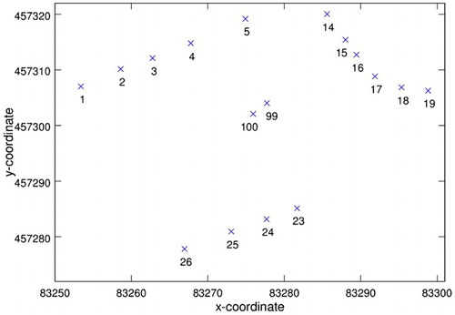
Three monumental buildings are monitored by total station measurements. Because of underground works, movements of the buildings might occur. Fifteen points are monitored (Fig. 1) from an instrument point that is not monumented and varies from epoch to epoch. Two epochs are considered (99 and 100 are the instrument points). A state-of-the-art high precision total station is supposed to have been used. The standard deviation of horizontal and vertical direction measurements is 0·3 mgon, of distance measurements 1 mm. The precision with which a point is defined (idealisation precision) is supposed to be 0·5 mm. The generated observations are listed in the appendix. The second epoch has two different lists of observations. In the first one (called case 1 hereafter) a deformation of point 1 is intentionally introduced. In the second one (case 2) the first five points, belonging to one building, are deformed.

1 Location of points

The generated observations were processed by the commercial software package MOVE3 (2014), version 4.2.1(×64). 3D coordinates and their full covariance matrix were computed. The covariance matrices of both epochs were defined relative to the approximate x-, y-, z-coordinates of point 1and 14 and z-coordinate of point 26. Note, however, that the testing results of the adjustment model of this paper are invariant to a change of base points. This was confirmed by computations with other base points. The approximate coordinates of the first epoch were in the national grid, those of the second epoch in a local system that was rotated on purpose over 100 gon relative to the national grid.

The adjusted coordinates and their covariance matrix, of both epochs, were transformed to the system of the first epoch and adjusted and tested with the adjustment model of this paper. A similarity transformation was used, in accordance with the degrees of freedom of the adjustments of each epoch in MOVE3. To do the computations a specifically designed Matlab programme was used. The results are shown in the appendix.

The covariance matrices of both epochs are rank deficient, because they are defined relative to a subset of the points. This results in a rank deficiency of 14 for the cofactor matrix of (8). Regularisation of the cofactor matrix has been used to handle the rank deficiency.

To estimate the parameters of the 3D similarity transformation and to adjust the coordinates, three computations (i.e. two iterations) were needed. In the last iteration the absolute value of the largest correction to the estimated parameters was less than 10⁻¹².

Testing of case 1

In case 1 a deformation of point 1 of 5·2 mm was induced by giving the x-, y- and z-coordinate each a bias of 3 mm.

The overall model test (F-test) of the adjustment yielded an F-value of 1·41, which was more than the critical value of 1·18 (computed with a one-dimensional significance level of 0·1%, a power of 80% and using the B-method of testing). Conventional w-tests were performed, using (60) and (61). None led to any rejection. Also point tests were performed, using (62). A point test is a three-dimensional test, where the alternative hypothesis is, that three independent biases are present for respectively the x-, y- and z-coordinate of a point. Point 1 was rejected with estimated errors (computed with (58)) of 4, 2 and 3 mm in resp. the x-, y- and z-direction of system r_a. This shows that using weighted least squares with full covariance matrices and applying a three-dimensional point test is capable of detecting deformed single points.

Point 1 is one of the base points that were held fixed on their approximate values in the epoch adjustments. Testing of this point, however, can be done with the model of this paper like the testing of the non-base points, without any additional action. This is possible, because the model includes a transformation. The estimated least squares residuals from ê of (46) are zero for the base points, but the reciprocal least squares residuals from of (47) are not. The reciprocal residuals are used for testing (56), (59) and (60)).

Testing of case 2

In case 2 the first five points, belonging to one building, are deformed, all with the same deformation: 3 mm along the x- and y-axis, −2 mm along the z-axis. The x-, y- and z-axis are those of the local system of the second epoch.

The overall model test (F-test) of the adjustment yielded an F-value of 2·20, which was more than the critical value of 1·18. Both conventional w-tests and point tests were performed. Only the w-tests of the x-coordinate of point 5 and the y-coordinate of point 2 led to rejection. Points 2 and 5 were rejected by the point tests. If, however, the deformation of this one building was tested by formulating an alternative hypothesis that the five points of this building had undergone the same deformation, the pertinent test led to rejection with a test statistic that was 2·01 times larger than the critical value. This was larger than the same ratio for any other alternative hypothesis that was formulated. The estimated deformation was 3, 3 and −4 mm in the direction of respectively the x-, y- and z-axis in system r_b. This shows that using weighted least squares with full covariance matrices and applying more-dimensional tests gives the possibility to detect deformations that are below the noise level of individual points.

Conclusions

The problem of finding the relation between two Cartesian coordinate vectors that pertain to the same points of an object under deformation, is addressed. If the two vectors refer to two different epochs, the relation between them is determined by a possible difference in geodetic datum, by a possible deformation, which may have occurred between both epochs, and by measurement noise. In this paper the relation is considered as describable by in principle one or more affine, congruence or similarity transformations, to be extended by other parameters.

An adjustment model is given to estimate the parameters of an affine, a congruence or a similarity transformation. The congruence and similarity transformation are formulated as an affine transformation with constraints. That makes it possible to avoid the use of Euler angles.

To compute approximate values for the parameters of a congruence and similarity transformation it is possible to compute first approximate values for an affine transformation and subsequently to change these values to those of a congruence or similarity transformation by applying a singular value decomposition of the rotation matrix. This computation of approximate values has to be repeated in each iteration step of solving the linearised adjustment model.

Applying the proposed linearised adjustment model with constraints makes it easy to extend the model as follows

1	Several transformations can be combined.
2	Different geodetic datums are taken account of.
3	Testing for biases in the coordinate vectors is made possible.
4	Testing alternative deformation models is possible.

The proposed linearised adjustment model can be solved to get a weighted least squares solution, where full covariance matrices of the coordinates of both epochs are taken account of. The covariance matrices may be singular positive semidefinite matrices.

The effectiveness of the proposed adjustment model is demonstrated in an experiment, where artificially added deformations are successfully detected.

Extending the proposed linearised adjustment model to more than two epochs and to more complex deformation models is straightforward.

Appendix

Conventions

In this paper use is made of the following conventions:

•	T indicates the transpose of a matrix
•	approximate values of a scalar or vector are indicated by a sub or super script 0, e.g. a scalar s0 or a vector v0
•	if v is a certain vector, then Δv is the vector of differences of v with its vector v0 of approximate values

For a scalar an analogous equation holds.

•	a vector that contains the coordinates of n points contains first all x-coordinates from point 1 up to point n, then all y-coordinates and finally all z-coordinates
•	the vector a consists of three sub vectors x, y and z, and the vector b′ of three sub vectors u, v and w, such that (40)
•	vector x contains for each point the x-coordinates. If there are n points, then (41)

In the same way y , z and u , v , w are defined.

Adjustment equations

Most of the following equations can be found in (Teunissen, 1999) and (Teunissen, 2006). To write the equations more concisely, and because of their central role in testing, the reciprocal least squares residuals are introduced.

A system of linear or linearised observation equations has the following general structure (42) where is the m-vector of observations, A is the (m×n)-matrix of coefficients and p is the n-vector of unknown parameters. The equation behind the semicolon describes the stochastic model by giving the covariance matrix , the variance factor σ² and the cofactor matrix Q _ℓ . Both A and Q _ℓ are considered in the following equations to be regular matrices. The situation that Q_λ is singular is treated in the paper.

The least squares solution is given by (43) (44) with the vector of estimated parameters and its cofactor matrix. We have also (45) (46) (47) with the adjusted observations, the least squares residuals and the reciprocal least squares residuals. The Q-matrices are their cofactor matrices. The reciprocal least squares residuals are used in the testing equations.

For each system of linear observation equations an equivalent system of linear condition equations exists (48) where K^T is the ((m-n)×m)-matrix of conditions, for which holds (Teunissen, 1999, p. 63) (49)

Matrix K is considered a regular matrix. is considered a positive semidefinite matrix, so it may be singular.

Define the vector of misclosures t and its cofactor matrix Q _t as (50)

The least squares solution is (51) (52) (53)

Testing equations

Consider models (42) or (48) as the null hypothesis. Let an alternative hypothesis be defined as (54) with G a (m×q)-matrix of known coefficients and ▿ a q-vector of unknown bias parameters, with m the amount of observations and q the amount of bias parameters. The formulation for the model of condition equations is (55)

To test this alternative hypothesis against the null hypothesis (model (42) or (48)) use is made of the following test statistic (Teunissen, 2006, p.78) (56) (57) with F_crit the critical value, the null hypothesis is rejected in favour of the alternative hypothesis.

If the null hypothesis is rejected, an estimate of the biases and its cofactor matrix can be determined as (Teunissen, 2006, p. 76) (58)

For q we have 1≤q≤m – n. If q>m – n the adjustment models (54) and (55) are underdetermined and cannot be solved. For the limiting case q = m–n the test is equal to the overall model test and we have (59)

The rightmost expression can be used if the system of condition equations is used and Q _ℓ is singular.

The limiting case q = 1 is the test of w-quantities (Baarda, 1968, p.13). It is called a w-test (60) reject the null hypothesis. Here w_crit is the critical value and g is the matrix G, but written as a lower case letter, because it has only one column: it is a vector. The w-quantity has a normal distribution with an expectation of 0 and a standard deviation of 1. A conventional w-test (Baarda, 1968, p.15) is the test of one observation being biased and all other observations being without bias. The vector g is (61) with the 1 corresponding to the biased observation.

A point test is a three-dimensional test (q = 3) of the x-, y- and z-coordinate of one point (used as observations). The matrix G is (62) with the ones corresponding to the coordinates that are supposed to be biased.

Point 1 is biased

Data of experimental validation

Observations of the first epoch
pnt	pnt	Direction	Distance	Zenith angle
99	1	307·7820765	24·5060074	99·8055455
99	2	319·7344105	20·0876102	98·7070717
99	3	331·5296877	17·0625166	105·4327481
99	4	352·4563301	14·7326649	106·6349756
99	5	388·3056469	15·4070803	101·3380122
99	14	29·0918416	17·8292985	99·7871557
99	15	46·7749502	15·3559925	96·6129838
99	16	59·3812951	14·5848606	99·6001975
99	17	79·1592740	14·9923557	105·715829
99	18	89·8716178	17·9265803	106·5598073
99	19	93·2971810	21·2104291	98·4820515
99	23	186·8788155	19·3414323	103·9408223
99	24	200·1056248	20·9264019	105·3692816
99	25	212·6876307	23·5421679	99·0553208
99	26	224·8455986	28·3270008	98·4196188

Observations of the second epoch, point 1 is biased
pnt	pnt	Direction	Distance	Zenith angle
100	1	13·7372731	23·0672793	99·7859602
100	2	27·7594635	19·1262636	98·6398106
100	3	41·4401419	16·6097400	105,582282
100	4	63·6494039	15·1749445	106·4430463
100	5	96·2060486	17·1252428	101·2017896
100	14	131·4346394	20·3808279	99·8127807
100	15	146·8624786	18·0020637	97·1040642
100	16	157·5422153	17·1916389	99·6580831
100	17	174·4918375	17·3543574	104·9366243
100	18	184·6390687	20·0631725	105·8611633
100	19	188·5080762	23·2655969	98·6169971
100	23	279·1965362	17·9334770	104·2543189
100	24	294·0907282	19·0647202	105·8937977
100	25	308·5860882	21·3237391	98·9581652
100	26	322·5863556	25·8583270	98·2684568

Observations of the second epoch, points 1 up to 5 are biased
pnt	pnt	Direction	Distance	Zenith angle
100	1	13·7372731	23·0672631	99·7997607
100	2	27·7642973	19·1302064	98·6467483
100	3	41·4423295	16·6141034	105·5885051
100	4	63·6455986	15·1792709	106·4496345
100	5	96·1955807	17·1284537	101·2089988
100	14	131·4346394	20·3808279	99·8127807
100	15	146·8624786	18·0020637	97·1040642
100	16	157·5422153	17·1916389	99·6580831
100	17	174·4918375	17·3543574	104·9366243
100	18	184·6390687	20·0631725	105·8611633
100	19	188·5080762	23·2655969	98·6169971
100	23	279·1965362	17·9334770	104·2543189
100	24	294·0907282	19·0647202	105·8937977
100	25	308·5860882	21·3237391	98·9581652
100	26	322·5863556	25·8583270	98·2684568

Approximate coordinates of the first epoch
pnt	x	y	z
099	83 277·7360	457 303·9790	2·0000
001	83 253·4140	457 306·9670	2·0740
002	83 258·6090	457 310·1060	2·4080
003	83 262·7790	457 312·0580	0·5460
004	83 267·7820	457 314·7330	0·4670
005	83 274·9220	457 319·1230	1·6760
014	83 285·6020	457 319·9780	2·0600
015	83 288·0160	457 315·3580	2·8170
016	83 289·4500	457 312·6660	2·0920
017	83 291·8750	457 308·7800	0·6560
018	83 295·3420	457 306·8040	0·1560
019	83 298·8230	457 306·2070	2·5050
023	83 281·6860	457 285·0840	0·8030
024	83 277·7020	457 283·1290	0·2370
025	83 273·0750	457 280·9050	2·3490
026	83 266·9620	457 277·7910	2·7030

Approximate coordinates of the second epoch
pnt	x	y	z
100	0·0000	0·0000	0·0000
1	4·9360	22·5280	0·0740
2	80·750	173·330	0·4080
3	100·270	131·630	−14·540
4	127·020	81·600	−15·330
5	170·920	10·200	−0·3240
14	17·9470	−9·6600	0·0600
15	133·270	−120·740	0·8170
16	106·350	−135·080	0·0920
17	67·490	−159·330	−13·440
18	47·730	−194·000	−18·440
19	41·760	−228·810	0·5050
23	−169·470	−57·440	−11·970
24	−189·020	−17·600	−17·630
25	−211·260	28·670	0·3490
26	−242·400	89·800	0·7030

dx, dy, dz = 3 mm, -3 mm, -3 mm

Observations of the second epoch, point 1 is biased

pnt	pnt	Direction	Distance	Zenith angle
100	1	13·7372731	23·0672793	99·7859602
100	2	27·7594635	19·1262636	98·6398106
100	3	41·4401419	16·6097400	105,582282
100	4	63·6494039	15·1749445	106·4430463
100	5	96·2060486	17·1252428	101·2017896
100	14	131·4346394	20·3808279	99·8127807
100	15	146·8624786	18·0020637	97·1040642
100	16	157·5422153	17·1916389	99·6580831
100	17	174·4918375	17·3543574	104·9366243
100	18	184·6390687	20·0631725	105·8611633
100	19	188·5080762	23·2655969	98·6169971
100	23	279·1965362	17·9334770	104·2543189
100	24	294·0907282	19·0647202	105·8937977
100	25	308·5860882	21·3237391	98·9581652
100	26	322·5863556	25·8583270	98·2684568

Observations of the second epoch, points 1 up to 5 are biased

pnt	pnt	Direction	Distance	Zenith angle
100	1	13·7372731	23·0672631	99·7997607
100	2	27·7642973	19·1302064	98·6467483
100	3	41·4423295	16·6141034	105·5885051
100	4	63·6455986	15·1792709	106·4496345
100	5	96·1955807	17·1284537	101·2089988
100	14	131·4346394	20·3808279	99·8127807
100	15	146·8624786	18·0020637	97·1040642
100	16	157·5422153	17·1916389	99·6580831
100	17	174·4918375	17·3543574	104·9366243
100	18	184·6390687	20·0631725	105·8611633
100	19	188·5080762	23·2655969	98·6169971
100	23	279·1965362	17·9334770	104·2543189
100	24	294·0907282	19·0647202	105·8937977
100	25	308·5860882	21·3237391	98·9581652
100	26	322·5863556	25·8583270	98·2684568

Approximate coordinates of the first epoch

pnt	x	y	z
099	83 277·7360	457 303·9790	2·0000
001	83 253·4140	457 306·9670	2·0740
002	83 258·6090	457 310·1060	2·4080
003	83 262·7790	457 312·0580	0·5460
004	83 267·7820	457 314·7330	0·4670
005	83 274·9220	457 319·1230	1·6760
014	83 285·6020	457 319·9780	2·0600
015	83 288·0160	457 315·3580	2·8170
016	83 289·4500	457 312·6660	2·0920
017	83 291·8750	457 308·7800	0·6560
018	83 295·3420	457 306·8040	0·1560
019	83 298·8230	457 306·2070	2·5050
023	83 281·6860	457 285·0840	0·8030
024	83 277·7020	457 283·1290	0·2370
025	83 273·0750	457 280·9050	2·3490
026	83 266·9620	457 277·7910	2·7030

Approximate coordinates of the second epoch

pnt	x	y	z
100	0·0000	0·0000	0·0000
1	4·9360	22·5280	0·0740
2	80·750	173·330	0·4080
3	100·270	131·630	−14·540
4	127·020	81·600	−15·330
5	170·920	10·200	−0·3240
14	17·9470	−9·6600	0·0600
15	133·270	−120·740	0·8170
16	106·350	−135·080	0·0920
17	67·490	−159·330	−13·440
18	47·730	−194·000	−18·440
19	41·760	−228·810	0·5050
23	−169·470	−57·440	−11·970
24	−189·020	−17·600	−17·630
25	−211·260	28·670	0·3490
26	−242·400	89·800	0·7030

Results case 1

Point 1 is biased

dx, dy, dz  =  3 mm, -3 mm, -3 mm

in x-system

Number_of_computations  =  3

Max_criterion  =  5·0e-013

Scale_factor  =  1

Translation_x_y_z_in_m  = 

    81475·939, 455202·030, 2·000

Alpha_Beta_Gamma_in_gon  = 

0, 0, -100

Overall model test:

    Number_of_conditions  =  38

    Ftest  =  1·41

    Critical_value  =  1·18

w-test: Critical value is 3·29

    No rejections

Point test: Critical value  =  4·21

    Point    F_q

    001    6·2758

    Est.def. x Est.def. y Est.def. z

    3·6 mm    -2·4 mm    -2·5 mm

Differences between x and adj. coord. in mm

1 0 0 0

2 -1·1 0·1 0·9

3 -1·6 1·5 1·2

4 -1·1 -0·2 1·1

5 -0·7 0·2 0·4

14 0 0 0

15 -1·1 -1·5 -1·1

16 -0·3 -0·6 -0·5

17 -0·9 -0·8 -0·4

18 -1·2 -1·7 -0·4

19 -2·1 -1·4 -0·6

23 -2·5 -1·1 0·0

24 -3·2 -1·5 -0·6

25 -2·9 0·9 0·0

26 -3·2 -0·5 0

Results case 2

Points 1, 2, 3, 4, 5 are biased

dx, dy, dz  =  3 mm, -3 mm, 2 mm

in x-system

Number_of_computations  =  3

Max_criterion  =  5·2e-012

Scale_factor  =  1

Translation_x_y_z_in_m  = 

    81475·940, 455202·029, 2·001

Alpha_Beta_Gamma_in_gon  = 

0, 0, -100

Overall model test

    Number_of_conditions  =  38

    Ftest  =  2·20

    Critical_value  =  1·18

w-test: Critical value is 3·29

x-coordinate

    Point Ratio w Est.error

    005   1·1582 3·8106 3·0011

y-coordinate

    Point Ratio w Est.error

    002   1·1816 3·8875 -3·2984

z-coordinate

    no rejections

Point test: Critical value  =  4·21

    Point   F_q

    002   5·8141

    Est.def. x Est.def. y Est.def. z

    2·3 mm -3·9 mm -0·4 mm

More-dimensional test

    q = 3, points 001, 002, 003, 004, 005

    F_q

    5·8141

    Est.def. x Est.def. y Est.def. z

    2·8 mm  -3·1 mm  3·7 mm

Differences between x and adj. coord. in mm

1 0 0 0

2 0·2 -1·2 -0·2

3 0·0 0·1 0·3

4 0·7 -1·7 0·6

5 1·0 -1·6 0·4

14 0 0 0

15 -1·2 -1·5 -0·6

16 -0·3 -0·7 0·2

17 -0·8 -0·9 0·7

18 -1·0 -1·9 1·1

19 -2·3 -1·4 1·2

23 -2·4 -1·2 1·1

24 -3·1 -1·7 0·2

25 -3·0 0·9 0·4

26 -3·4 -0·5 0

References

- Arun K. S., Huang T. S. and Blostein SD., 1987. Least-squares fitting of two 3-D point sets. IEEE Transactions on Pattern Analysis and Machine Intelligence, PAMI-9(5).
- Awange J. L., Fukuda Y. and Grafarend E., 2004. Exact solution of the non-linear 7-parameter datum transformation by Groebner basis. Bollettino di Geodesia e Scienze Affini, 63, pp.117–27.
- Baarda W., 1968. A testing procedure for use in geodetic networks. Publications on Geodesy, New Series 2(5) ed. Delft: Netherlands Geodetic Commission.
- Baarda W., 1995. Linking up spatial models in geodesy – extended S-transformations. Publications on Geodesy, New Series 41 red. Delft: Netherlands Geodetic Commission.
- Bakker G., de Munck J. C. and Strang van Hees GL., 1989. Radio positioning at sea: geodetic survey computations, least squares adjustment. Delft: Delft University Press.
- Fang X., 2011. Weighted total least squares solutions for applications in geodesy. Hannover: Leibniz Universität Hannover.
- Hanson M. J. and Norris RJ., 1981. Analysis of measurements based on the singular value decomposition. SIAM Journal on Scientific and Statistical Computing, 2(3), pp.363–73.
- Higham NJ., 1989. Matrix nearness problems and applications. In: M. Gover and S. Barnett, eds. Applications of matrix theory. Oxford: Oxford University Press. pp. 1–27.
- Hinsken L., 1987. Algorithmen zur Beschaffung von Näherungswerten für die Orientierung von beliebig im Raum angeordneten Strahlenbündeln. PhD. Series C Nr.333. München: Deutsche Geodätische Kommision.
- Hofmann-Wellenhof H., Lichtenegger H. and Collins J., 2001. Global positioning system: theory and practice. 5th ed. Wien New York: Springer-Verlag.
- Horn BKP, Hilden H. M. and Negahdaripour S., 1988. Closed-form solution of absolute orientation using orthonormal matrices. Journal of the Optical Society of America, 5, pp.1127–35.
- Krarup T., 2006. Contribution to the geometry of the helmert transformation. In: K. Borre, ed. Mathematical foundation of geodesy: selected papers of torben krarup, pp. 359–74. Berlin: Springer.
- MOVE3, 2014. MOVE3. [Online]. Available at: http://www.move3.com/ [Accessed 4 July 2014].
- Schut G.H, 1960/61. On exact linear equations for the computation of the rotational elements of absolute orientation. Photogrammetria, 1, pp.34–37.
- Snow K., 2012. Topics in total least-squares adjustment within the errors-in-variables model: singular cofactor matrices and prior information. Columbus, OH: Ohio State University.
- Strang G., 1988. Linear algebra and its applications. 3rd ed. San Diego: Harcourt Brace Jovanovich.
- Teunissen PJG., 1985. The geometry of geodetic inverse linear mapping and non-linear adjustment. Publications on Geodesy New Series, vol. 8, no. 1 ed. Delft: Netherlands Geodetic Commission.
- Teunissen PJG., 1999. Adjustment theory; an introduction. Delft: Delft University Press.
- Teunissen PJG., 2006. Testing theory; an introduction. Delft: Delft University Press.
- Teunissen PJG, Salzmann M. A. and de Heus HM., 1987. Over het aansluiten van puntenvelden: De aansluitingsvereffening. NGT Geodesia, 29(6/7).
- Thompson EH., 1959. An exact linear solution of the problem of absolute orientation. Photogrammetria, 4, pp.163–78.
- Tienstra JM., 1956. Theory of the adjustment of normally distributed observations. Amsterdam: Argus.
- Tienstra M., 1969. A method for the calculation of orthogonal transformation matrices and its application to photogrammetry and other disciplines. Ph. D. Delft University of Technology.
- Wolf H., 1982. Alternate use of restriction equations in Gauss-Markoff adjustments. In: Forty Years of Thought... Anniversary edition on the occasion of the 65th birthday of Professor W. Baarda 1. pp. 194–200. Delft
- Xu P., Shimada S., Fujii Y. and Tanaka T., 2000. Invariant geodynamical information in geometric geodetic measurements. International Journal of Geophysics, 142, pp.586–602.