Comparative analysis of trip generation models: results using home-based work trips in the Seoul metropolitan area

Abstract

This paper compares the performance of trip generation models. Trip generation estimates the number of trips to and from a traffic analysis zone. This process is the first stage of the conventional four-step travel forecasting framework. Although many approaches have been suggested for this step, regression and category analyses have been widely applied. The two methods have generated an acceptable level of performance from the perspective of transport planning. Critical problems, however, have also been observed. In the regression analysis, trip rates are treated as continuous variables that can be negative, which is obviously unrealistic. Furthermore, the method does not incorporate traveler behavior. For the category analysis, its arbitrary way of choosing independent variables and their strata has drawn critiques. The cell-by-cell calculation in this method also increases the concerns about unreliable estimation of trip rates. Censored regression, count data, and discrete choice models have been visited for the alternative of regression approach while the multiple classification method has been conceived for the substitute of the category analysis. A systematic examination of the performance among the models has not been discussed sufficiently yet, which is the motive of this paper. Six representative models – regression, tobit, Poisson, ordered logit, category, and multiple classification analyses – were applied to the home-based work trips in the Seoul metropolitan area. Cross-validation and back-casting were the key for checking the performance among the models. In this process, the measures of correlation, variance, and coincidence were compared. The category-type model was superior in overall performance.

Keywords:

• Trip generation
• Regression model
• Tobit model
• Poisson model
• Ordered logit model
• Cross-classification
• Multiple classification analysis
• Validation

Introduction

This paper compares the performance of trip generation models. Trip generation, which is the first phase of conventional four-step travel forecasting framework, estimates the number of trips to and from each traffic analysis zone (TAZ) for various purposes. This trip-based traditional approach is still the standard practice for most strategic transport planning, even though advanced approaches like tour- and activity-based models explore more realistic representations of behavior in travel demand studies (McNally and Rindt, 2007; Donnelly et al., 2010).

The trip generation estimation procedure employs mathematical models that associate each purpose with demographic characteristics of the TAZ, such as population, households, employment, vehicle ownership, and income. Current information on these variables may be obtained from household surveys or census reports. Future information, on the other hand, is derived from projections.

Early versions of trip generation were mainly based on zonal aggregation approaches. However, the aggregate models lack the context of travelers’ behavior. Household-based schemes, thus, are more common in current practice, even though they require an additional process of obtaining zone-level totals (Papacostas and Prevedouros, 2001; 351–353).

Linear regression (hereafter regression) and category analyses are the representative methodologies used for this step. They have widely been applied to empirical studies and may have shown acceptable performance from the planning perspective.

However, there are also limitations of these traditional frameworks. For regression-based trip generation models, three typical drawbacks have been observed. First, the number of trips is treated as a continuous random variable though it is a discrete one (Barmby and Doornik, 1989; Ma and Goulias, 1999; Wallace et al., 1999; Jang, 2005; Schmöcker et al., 2005; Badoe, 2007; Roorda et al., 2010; Lim and Srinivasan, 2011). People, for example, can make two trips per day; people cannot make 1·7 trips per day. Second, the dependent variable may take on negative values due to the assumption of normal distribution for the disturbance of trip rates (Barmby and Doornik, 1989; Cotrus et al., 2005; Ma and Goulias, 1999; Wallace et al., 1999; Jang, 2005; Badoe, 2007). In trip generation, the dependent variable is zero for a significant fraction of the observations. For those who make trips, the travel demand can be measured; but for those who do not, the spatial interaction cannot be recorded and is set equal to zero. Namely, although the data for trip generation are censored, the regression model cannot address the nature. Finally, the model does not represent traveler behavior theory because it simply matches a statistical relationship between the dependent variable and a set of independent variables (Schmöcker et al., 2005; Badoe, 2007; Roorda et al., 2010; Lim and Srinivasan, 2011). It is difficult to observe travelers’ behavioral mechanisms in trip-making, such as utility maximization and cost minimization. The category analysis may have useful advantages over regression-type trip generation models (Stopher and McDonald, 1983). The technique is independent upon the zonal system of the study area; no assumptions are required about the shape of the relationship between the trip rate and explanatory variables; it represents class-specific behavior; and it does not permit extrapolation beyond its calibration strata, although the lowest or highest class of a variable can be open-ended. However, the model also suffers from two broad limitations (Stopher and McDonald, 1983). First, a naïve approach in choosing independent variables and their strata for classification is not statistically justifiable but only empirically acceptable. The method bears no statistical goodness-of-fit measures, so the calibration cannot be verified. Second, the cell-by-cell calculation reduces the reliability of cell values. In particular, the uncertainty increases when there are cells with small samples and/or large variances. This calculation mechanism also requires large sample sizes, which incurs much cost and time (Ortúzar and Willumsen, 2011; 158).

There has been research to overcome and/or mitigate these limitations. Censored regression models such as tobit analysis have been used to block the potential negative values on trip generation rates (Cotrus et al., 2005). Poisson and negative binomial models have been used to try to address the integer nature of the dependent variable (Barmby and Doornik, 1989; Ma and Goulias, 1999; Wallace et al., 1999; Jang, 2005; Badoe, 2007). These count data models can also confine the figure of the trip rate greater than or equal to zero. Ordered logit and probit models can be understood as generalized frameworks in regression-based trip generation modeling since the discrete choice methods are, in principle, free from the three limitations of the likelihood of negative trip rates, the continuous dependent variable, and the lack of incorporation of traveler behavior theory (Sheffi, 1979; Agyemang-Duah and Hall, 1997; Schmöcker et al., 2005; Badoe, 2007; Roorda et al., 2010). Multiple classification analysis is also found in the literature as an alternative approach to a simple category model for person trips (Stopher and McDonald, 1983) and for freight movements (Bastida and Holguin-Veras, 2009). This model adopts a statistically justifiable approach based on analysis of variance (ANOVA). The cell value is estimated with the grand and group means (Stopher and McDonald, 1983).

As reviewed, there have been studies to alleviate the limitations of conventional trip generation models. Also, some literature has compared two models (e.g., Cotrus et al., 2005) or more (e.g. Badoe, 2007; Lim and Srinivasan, 2011). The comparative studies, however, have mostly focused on the estimation results and a rough validation, normally with current datasets. On the other hand, a systematic validation is explored in this study to compare the performance of models, incorporating both cross-validation and the historical method in the form of back-casting. It should be noted that the model comparison does not directly ascertain whether the forecast response is correct, but does assess whether it is reasonable or explainable given what is known about traveler behavior.

The next section describes the scope and design of this study. Subsequent two sections deal with the theoretical basis of the trip generation models which are tested in this paper. The process and results of the empirical study then follow. The section includes data used, estimation results, and performance comparison of the models. Finally, concluding remarks are given.

Scope and design

Figure 1 summarizes the critiques on the conventional trip generation models as discussed in the introductory section. The diagram also shows the alternative approaches and their representative models, for which performance is tested in this paper.

1. Conventional approaches and their alternatives

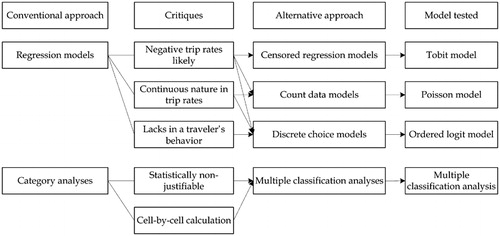
In fact there are other models for each group of alternatives. The ordered probit (Schmöcker et al., 2005; Roorda et al., 2010; Lim and Srinivasan, 2011), the negative binomial (Wallace et al., 1999; Badoe, 2007; Lim and Srinivasan, 2011), and the truncated normal (Badoe, 2007) models have been applied from the groups of discrete choice, count data, and censored regression frameworks, respectively. However, they are less common methodologies than those chosen in Figure 1.

It should also be noted that there are approaches which are not included in this comparative study. Highly sophisticated techniques such as the count data model with zero inflation (Jang, 2005) and the two-limit tobit version are not included in this study. The binary stop-go model (Daly, 1997) is not considered either. There may be others which are not enumerated in this paper. Indeed, these advanced models are associated with appealing theoretical structures. However, their corresponding empirical performances have not generally been verified.

Regression-type models

Regression model

Regression analysis in trip generation functionalizes the relationship between trip generation rates, or the dependent variable, and a set of independent variables(1) where is the trip generation rate, n indexes the nth observation (which is households in this study), β is the vector of parameters that should be estimated, x is the vector of independent variables, and ϵ is a random disturbance.

Regression models require rather strong assumptions. Four representative issues are that the linear functional form is demanded; the model parameters should be identifiable, namely the full rank condition should be satisfied; the data on the independent variables are non-stochastic; and the disturbances are normally distributed, with zero mean and constant (or homoscedastic) and uncorrelated (or independent) variance (Greene, 2000; 213–223).

Tobit model

Only the part of the distribution above  = 0 is relevant to the modeling for trip generation. Conventional regression methods fail to account for the qualitative difference between limit (zero) and non-limit (continuous) observations. The tobit model is a useful tool to deal with these censored data. When data are censored, the distribution that applies to the sample data is a mixture of discrete and continuous distributions (Cotrus et al., 2005). To analyze this distribution, a new random variable q which is transformed from the original is defined(2)

The result of the partial derivative with respect to any independent variable cannot be the marginal effect of the variable, since is unobserved. The marginal effect in this kind of model, or the case with censoring at zero and normally distributed disturbances, is given by(3) where Φ(⋅) is a normal cumulative distribution function and σ is the standard deviation of the error term (Greene, 2000; 905–926).

Poisson model

Trip rates, or the dependent variable, clearly show a discrete nature. In addition, a very large proportion of trip rates by households are zeros or small values. Regression analyses based on least squares hold limitations for dealing with these characteristics. A count data model such as a Poisson regression can be an alternative framework(4) where P(⋅) is the probability, the log-linear function is normally applied to λ_n, namely ln λ_n = β^Tx_n, and the partial effects in this non-linear regression model are given by λ_nβ (Greene, 2000; 880–893).

The Poisson model, however, shows a critical limitation: it assumes that the conditional mean and variance functions are equal. Overdispersion is particularly problematic (Barmby and Doornik, 1989; Ma and Goulias, 1999; Wallace et al., 1999; Jang, 2005; Badoe, 2007). If overdispersion is detected, the negative binomial model, which considers the variance to differ from the mean, is usually considered to apply. However, the data used for this study are not very concerned with this problem, as shown in Table 2.

Table 2. Number of households by trip rate

	Data in 2006			Data in 2002
Trip rate	Total	Estimation set	Validation set	Validation set
0	43 521 (20·57)	30 455 (20·57)	13 066 (20·59)	29 237 (18·38)
1	115 358 (54·53)	80 738 (54·52)	34 620 (54·54)	91 139 (57·30)
2	43 714 (20·66)	30 616 (20·67)	13 098 (20·64)	31 504 (19·81)
3	7630 (3·61)	5337 (3·60)	2293 (3·61)	5961 (3·75)
4	1234 (0·58)	872 (0·59)	362 (0·57)	1126 (0·71)
5 or more	107 (0·05)	73 (0·05)	34 (0·05)	101 (0·06)
Total	211 564 (100·00)	148 091 (100·00)	63 473 (100·00)	159 068 (100·00)
Average	1·1130	1·0928	1·0920	1·0926
Standard deviation	0·7702	0·7804	0·7799	0·7802

The number in parentheses refers to the percentage; return-home trips are excluded since origin-destination-based data are only available in 2002 while production-attraction-based data are also built in 2006.

Ordered logit model

The observed number of trips made by households is ordered. The count data model explains these rates using a definite point value. However, it would be more natural to think that a decision-maker has some level of utility associated with trip-making. When the level of utility is above some cutoff values, it is understood to lead to trip-making.

The ordered logit model specifies trip rates as a set of ordered alternatives. It is not difficult to regard that one alternative is similar to those close to it and less similar to those further away (Train, 2009; 159–164)(5) where θs are cutoff points for the possible responses and has the similar specification to the other models in this study, namely .

Provided that ϵ_n is distributed logistic, the probability of household n making k trips is given by(6) where F(⋅) is the cumulative distribution function of ϵ_n.

The marginal effects of the ordered logit model is given by(7) where F′(⋅) is the logistic density function and thus the effects represent the rate of change in the probability of trip-makings associated with a unit change in the independent variables, holding all other variables constant.

Cross-classification-type models

Category analysis

The category analysis, or the cross-classification method, would be the most extensively used approach for trip generation. In this framework, household types are classified according to a set of categories that are highly correlated with trip-making. The dependent variable is assumed to be continuous and two or three explanatory variables, each broken into three or four discrete levels, are usually applied. The independent variables can include household size, car ownership, household income, and some measures of land-use.

Mathematically, each household category constitutes a cell in the cross tabulation. The average trip rate in a cell is then calculated by simple algebra(8) where is the average number of trips made by household type h (e.g., the one car and two-worker household); Q_h and H_h are the total number of trips and households observed for type h, respectively.

Multiple classification

The conventional category analysis suffers from two important methodological drawbacks: a non-statistical basis and cell-by-cell calculation. The multiple classification method can overcome these disadvantages. A statistically justifiable approach based on a series of ANOVAs is applied to select independent variables and their strata. First, one-way ANOVAs between trip rates and each candidate variable are used to find the best grouping for each variable. In this process, measures such as an F statistic and R² can be used. Once statistically significant independent variables have been identified, multi-way ANOVAs between trip rates and two or three candidate variables are applied. It is an extensive trial-and-error procedure to examine the best classification scheme. The eta-square η², which is the ratio of the sum of squares of the candidate variable to the corrected total in the ANOVA output, can be used to determine more contributable variables (Stopher and McDonald, 1983). A grand-group mean approach is used to estimate the cell value. The grand mean is calculated over the entire sample, while the group mean is computed from the row and column sums of the category table. A cell value is found by adding the deviations of the cell to the grand mean; this process is different from the cell-by-cell calculation in the conventional category analysis (Stopher and McDonald, 1983).

There are two drawbacks to multiple classification analysis. The ANOVA-based statistically justifiable approach requires extensive trial-and-error procedures with no claim of optimality. Its empirical acceptance is subject to low efficiency in selecting good classification structures. The grand-group mean calculation also loses the class-to-class relationship between independent variables since one variable is computed over all classes of the other variable (Stopher and McDonald, 1983).

Method for model comparison

Schemes

The goodness-of-fit for each model are examined based on several procedures: the signs of the variables are checked against engineering judgment and corresponding expectations; a t-test based on the standard error of the estimate is applied to inspect the statistical significance of each variable; a statistic which is used for exploring the significance of the entire model is estimated, such as the F-statistic for the regression analysis and the likelihood ratio test for the ordered logit model; and informal indicators such as the coefficient of determination R² and McFadden’s ρ² are examined.

However, the comparison between models is not straightforward. The magnitude of the estimated coefficients cannot be meaningfully compared between the models since the scales are different. The same holds true for the standard goodness-of-fit measures such as the F-test, R², and t-test.

The performance comparison between models is conducted with validation. Validation tests a model’s ability to predict future behavior. It requires comparing the model output with information other than that used in estimating or calibrating the model. Namely, the model output is compared with observed travel data. Two ways of checking model performance are considered in this paper. They are the historical method and cross-validation.

Cross-validation is a statistical method for validating a predictive model. Subsets of the data are held out for use as validating sets; a model is fit to the remaining data and used to predict for the validation set. Averaging the quality of the predictions across the validation sets yields an overall measure of prediction accuracy.

There are three distinct forms in the cross-validation. Table 1 summarizes the advantages and limitations of the cross-validation techniques. The simplest type would be the hold-out technique, which is adopted in this study. It divides observations into two subsets: one is for estimation and calibration, and the other is for validation. Another form of cross-validation leaves out a single observation at a time; this is similar to the jackknife technique in the resampling. Lastly, the K-fold cross-validation technique splits the data into K subsets; each is held out in turn as the validation set (Picard and Cook, 1984; Kohavi, 1995).

Table 1. Advantages and limitations of the cross-validation methods

	Advantages	Limitations
Hold-out method	Easy to apply	Little reliable rule for the sample classification
K-fold method	Known to involve reasonable levels of errors	Little reliable rule for determining the number K
	Acceptable computational needs
Leave-one-out method	Minimal errors incurred in principle	Too much computational burden

The hold-out method is easy to apply, but there are few reliable rules for classifying samples into the estimation and validation sets. If data for estimation and validation are sufficient enough as in this study, this issue does not empirically matter much. The leave-one-out technique may incur minimal errors because it simulates total sample-size times, leaving just one observation out in every trial. However, this method is inapplicable to large sized datasets. The K-fold method requires acceptable computation time and may generate reasonable errors in the validation. However, this scheme also suffers from the arbitrariness in determining the number K.

The historical technique is either forecasting, in which a prior-year model is used to forecast current travel that is then compared with actual current travel, or back-casting, in which a current year model is used to estimate travel for a prior year that is then compared with actual travel in the prior year. The literature establishes little consensus on the better of the two: the choice is fundamentally data-dependent (Committee for Determination of the State of the Practice in Metropolitan Area Travel Forecasting, 2007). Using both trials, of course, would be good practice. In this paper, back-casting is used due to data availability.

Measures

It would be desirable to have some quantitative measures for validation. In this paper, measures of correlation, variance, and coincidence are considered (Cambridge Systematics, Inc., 2010).

Correlation refers to a statistical relationship between the observed and estimated trip rates. The closeness can be expressed numerically by the correlation coefficient r(9) where refers to the estimated value of , is the covariance between and , and and are the standard deviations of and , respectively.

Root-mean-square error (RMSE) is a measure of the differences between values predicted by a model and those actually observed(10)

Though RMSE is a good index of model accuracy, it is vulnerable to the scale problem. Per cent RMSE is an alternative because it is the normalized version of RMSE, removing scaling effects(11)

Low RMSEs and high values of the correlation coefficient are only one desirable measure of fit. Another important criterion is how the model simulates the pattern of the data. Namely, the distribution of estimated trip frequency should be analogous to the shape in the data. Thus, the ability to duplicate turning points or rapid changes in the data is an important criterion for model evaluation. The coincidence plot and its corresponding ratio are a useful tool to address this issue. The plot compares estimated and observed trip frequency distributions. The ratio measures the per cent of area that coincides. This rate lies between zero and one, where zero indicates two disjoint distributions and one means an identical pattern (Cambridge Systematics, Inc., 2010)(12) where H_k and are the total number of households observed and estimated at trip count k, respectively.

Empirical analysis

Data

The study area is the Seoul metropolitan region in Korea. The geographical sector includes Gyeonggi province; Incheon, which is the fourth largest city in Korea; and Seoul, the largest city and capital of the country. Sub-regions establish the functional relationships in terms of lifestyles, economic activities, urbanization, and land-uses.

There are two broad sets of data used in this study. The data for household characteristics and trip generation rates are based on the household travel diary survey of the Seoul metropolitan area. The Korea Regional Development Total Information System (REDIS) database supplies the regional characteristics that affect home-based work trips.

The Korea Regional Development Total Information System is the official statistical database of the Korea Presidential Committee on Regional Development. It collects more than 300 regional statistics and has provided the data to the public since 2008. This study has used four types of data: demographics, regional economy, transport system, and land-use.

The travel diary survey was started in 2002 by the code prescribed in the Korea Intermodal Surface Transportation Efficiency Act. This study extracted home-based work trips from data surveyed in 2002 and 2006. The data of 211 564 households in 2006 and those of 159 068 households in 2002 were collected, as shown in Table 2. Two-thirds of the data from 2006 were used for the estimation while the remaining data from 2006 and all the samples in 2002 were applied for the validation. Since the sample size of the ‘5 or more trip rate’ is too minimal compared to those of the others, the category was excluded in this study. Thus the sample size in Table 5 is 148 018 not 148 091.

Table 5. Estimation results for regression, tobit, Poisson, and ordered logit models

	Regression	Tobit	Poisson	Ordered logit
Constant	0·0098	−0·3352 (−0·3073)***	−0·9518 (−1·0383)***	−1·8605***
Number of employees	0·5394***	0·6166 (0·5652)***	0·4208 (0·4591)***	1·9776***
Household income	0·0947***	0·1303 (0·1194)***	0·1004 (0·1095)***	0·3307***
Car ownership	0·0072*	0·0323 (0·0296)***	0·0276 (0·0301)***	0·0469***
Population density	0·0022***	0·0031 (0·0028)***	0·0030 (0·0033)***	0·0063***
Annual expenditures per capita per area	0·3014***	0·2972 (0·2724)***	0·2878 (0·3139)**	0·9318***
Number of subway lines	0·0091***	0·0101 (0·0093)***	0·0068 (0·0075)	0·0314***
Number of companies per area	0·0551***	0·074 (0·0678)***	0·0432 (0·0471)***	0·1880***
σ		0·7248 (0·6644)***
Scale factor for marginal effects		0·9167	1·0909
θ1				3·5167***
θ2				6·4983***
θ3				9·0627***
Sample size	148 018	148 018	148 018	148 018
Estimator	OLS	MLE	MLE	MLE
F-statistic	68 367·6***
		75 740·6***	29 981·8***	77 142·6***
R^2	0·4005
ρ^2		0·1765	0·0828	0·2302

* 10% significance level; ** 5% significance level; *** 1% significance level; is the likelihood ratio statistic where L(0) is the value of the log likelihood function when all parameters are zero and is that at its maximum.

Estimation results

Table 3 shows the independent variables considered in the study. Three kinds of household characteristics and four sets of regional characteristics were considered.

Table 3. Independent variables considered

	Variable type	Variables considered
Household	Household composition	Number of telecommuters
characteristics		Number of employees
		Number of household members
		Number of preschool children
	Income level	Household income
		House ownership
	Transportation	Car ownership
		Number of cars owned
		Subway availability
		Number of household members with driving licenses
Regional	Demographics	Total population
characteristics		Population density
		Population moved in
		Population moved out
	Regional economy	Annual expenditures
		Annual expenditures per capita
		Annual expenditures per capita per area
		Annual tax revenues
		Annual local tax revenues
		Annual local tax per capita
		Fiscal self-reliance ratio
	Transport system	Number of car registered
		Number of car registered per capita
		Number of subway stations
		Number of subway lines
		Number of bus routes
		Road density
	Land-use	Gross area
		Residential area
		Commercial area
		Industrial area
		Green area
		Number of employees
		Number of employees per area
		Number of companies
		Number of companies per area

The specifications for regression, tobit, Poisson, and ordered logit models are shown in Table 4. These are the result of trial-and-error experiments for the modeling of trip generation, finding an empirically best fit for each approach. The process is subject to arbitrariness, but it cannot be avoided in comparing different models; note that the models tested have different mathematical structures. However, it should be stressed that the four models have the same independent variables through the heuristic method for specification, which is helpful for a fair comparison across the models tested.

Table 4. The specification for regression, tobit, Poisson, and ordered logit models

Variable	Specification
Dependent variable
Trip rates	Number of trips per household
Independent variables
Number of employees	Number of employees per household
Household income	1 if household income is below 1000 K won
	2 if household income ranges 1000–2000 K won
	3 if household income ranges 2000–3000 K won
	4 if household income is over 3000 K won
Car ownership	1 if a household has cars; 0 otherwise
Population density	1000 persons per square kilometer
Annual expenditures per capita per area	1000 K won per person per square kilometer
Number of subway lines	Number of lines within walking distance
Number of companies per area	1000 companies per square kilometer

Table 5 shows the estimation results for regression, tobit, Poisson, and ordered logit models. The results show satisfactory goodness-of-fit. The formal significance indices of F- and the likelihood ratio statistics indicate that the null hypothesis that all the parameters are zero can be rejected at the 0·01 level of significance. The values of R² and ρ², though they are an informal goodness-of-fit index, are also at an empirically acceptable level. However, the ρ² of the Poisson model is relatively low.

Not just the overall goodness-to-fit but also the reasonableness of each parameter should be checked. Since the marginal effects of independent variables are not equal to the coefficients in the tobit, Poisson, and ordered logit models, the effects are also given. The figures in the parentheses of Table 5 are the partial effects of parameters of the tobit and Poisson models while those for the ordered logit model are shown in Table 6. Even though the discussion regarding the partial effects is indirect to the purpose of this paper, the effects are useful for examining sensitivity to the explanatory variables.

Table 6. Marginal effects of ordered logit model

Independent variable	q = 0	q = 1	q = 2	q = 3	q = 4
Number of employees	−0·20249	−0·09550	0·27576	0·02048	0·00175
Household income	−0·03386	−0·01597	0·04611	0·00342	0·00029
Car ownership	−0·00480	−0·00227	0·00654	0·00049	0·00004
Population density	−0·00065	−0·00031	0·00088	0·00007	0·00001
Annual expenditures per capita per area	−0·09540	−0·04500	0·12993	0·00965	0·00082
Number of subway lines	−0·00322	−0·00152	0·00438	0·00033	0·00003
Number of companies per area	−0·01925	−0·00908	0·02621	0·00195	0·00017

All the coefficients in the model estimates have the expected signs. The variable ‘number of employees’ is the direct explanatory factor for the home-based work trips. It is common sense that more commuters make more commuting trips. This element, however, is not the only cause for trip generation. The variables ‘household income’ and ‘car ownership’ are the independent variables from the group of household characteristics. They reflect the degree of economic activities by household. Namely, it can be expected that a trip-maker with vehicles and higher income would actively participate in economic activities. This results in more spatial interactions in the form of commuting trips. The variable ‘number of subway lines’ is the factor of regional characteristics in terms of the transport system. Since the study area is the urbanized Seoul metropolitan region, this geographic sector suffers from the chronic congestion that other large cities normally do. Hence, households would prefer their residential locations close to public transportation. In particular, rail transport is known to be the most reliable travel mode in terms of travel time. Thus, the mandatory journey has a positive causality with transit proximity. The length of subway lines can also be considered as an alternative for the proximity variable. However, the aggregate measure would be restrictive to explain the number of options in rail travels that trip-makers face in their daily lives. The variables ‘population density’, ‘annual expenditures per capita per area’, and ‘number of companies per area’ from the categories of demographics, regional economy, and land-use are directly or indirectly related to employment opportunity. More companies can mean more jobs, which require more people. As a result, an area becomes denser. A local government normally earns more taxes in a region with large population, resulting in governments spending larger budgets.

The term ‘constant’, on the other hand, should be understood more carefully. It represents the disturbance in the model formulation. Thus, it should be read as the collective effects of the independent variables that are not included in the specification. Hence, the positive sign, as in the regression model, would match to the statistical background.

However, not all the coefficient estimates are significantly different from zero at the usual 5 or 1% levels of significance. Note that for most coefficients, the null hypothesis that the true value is zero can be rejected at the 1% significance level, but some others are not statistically different from zero at the same significance level. However, the inability to reject the hypothesis that some coefficients are zero at a particular significance level does not imply that the hypothesis must be accepted.

Table 7 shows the results of the traditional category analysis. The selection and stratification of independent variables of this scheme fundamentally follows an ad hoc procedure. The choice of explanatory factors comes from the result of the multiple classification analysis. The levels of household income are the same as the specification of the previous four models. Also, a simple increment for the grouping has been applied as in a usual category scheme. These designs allow for consistent performance comparison between the models tested.

Table 7. Average daily commuting trips per household by cross-classification

Population density	Household income	Number of employees
		0	1	2	3 or more
Low	0–1000 K won	0·26	0·47	0·76	1·37
	1000–2000 K won	0·69	0·76	1·27	1·52
	2000–3000 K won	0·87	0·84	1·48	1·98
	3000 K won or more	0·90	0·86	1·58	2·27
Medium	0–1000 K won	0·08	0·73	1·35	1·83
	1000–2000 K won	0·26	0·85	1·54	2·11
	2000–3000 K won	0·32	0·89	1·61	2·22
	3000 K won or more	0·41	0·90	1·66	2·39
High	0–1000 K won	0·11	0·74	1·36	1·93
	1000–2000 K won	0·33	0·85	1·53	2·18
	2000–3000 K won	0·39	0·91	1·60	2·33
	3000 K won or more	0·47	0·92	1·69	2·51

Table 8 is the summary of the one-way ANOVAs for the grouping of the independent variables for multi-category analysis. All the explanatory variables considered in the regression, tobit, Poisson, and ordered logit models also show statistical significance in this multivariate analysis.

Table 8. The result of one-way ANOVAs for the multiple classification analysis

Candidate variable	Stratification	F-statistic
Number of employees	0, 1, 2, and 3 or more	31541·922***
Household income	0–1000 K won, 1000–3000 K won, and 3000 K won or more	4647·556***
Car ownership	0 and 1 or more	1306·429***
Population density	Low (0–5000), medium (5000–18 000), and high (18 000 or more)	722·164***
Annual expenditures per capita per area	0–100, 100–200, 200–300, and 300 or more	58249·731***
Number of subway lines	0, 1, 2, 3, and 4	33·762***
Number of companies per area	0–500, 500–1000, and 1000 or more	285·863***

Population density, annual expenditures per capita per area, and number of companies per area are represented by persons per square kilometer, 1000 won per capita, and companies per square kilometer, respectively; and *** 1% significance level.

In general, two or three independent variables can be considered for this analysis in the form of two- or three-way ANOVAs, respectively. Since seven candidate variables are all statistically significant, the scheme requires a series of ANOVAs with a trial-and-error basis. The details of the extensive ANOVA runs are not provided in this paper: the result of the empirically best run, based on a three-way ANOVA, is given in Table 9.

Table 9. Average daily commuting trips per household by multiple classification

Population density	Household income	Number of employees
		0	1	2	3 or more
Low	0–1000 K won	0·07	0·10	0·69	1·18
	1000–3000 K won	0·52	0·54	1·13	1·63
	3000 K won or more	0·66	0·68	1·27	1·77
Medium	0–1000 K won	0·18	0·73	1·45	2·09
	1000–3000 K won	0·36	0·92	1·64	2·27
	3000 K won or more	0·43	0·99	1·71	2·34
High	0–1000 K won	0·31	0·82	1·53	2·25
	1000–3000 K won	0·50	1·00	1·71	2·44
	3000 K won or more	0·59	1·10	1·81	2·53
F-statistic	3237·538***
R^2	0·434

The cell values in the conventional and multiple cross-classifications generally match prior expectations. Namely, the trip rate increases as the income is higher and the number of employees grows. Two interesting observations, however, should be noted. First, two couples of cells that are shaded in the traditional category analysis contradict common sense. Intuitively, everything else being equal, the one-employee household can be expected to make more trips than the non-employee household. However, the outcome is the reverse. Meanwhile, the reason in which non-employee households make trips is that there can be employers in the household who contribute to the number of commuting trips. Second, the cell values in the conventional model are similar between the medium and high density areas. This may suggest that population density can be classified into low and a combined medium and high. It may also imply that the other independent variables are not very well stratified. Unfortunately, there is little systematic way to identify the cause in the conventional category analysis. The multiple classification has generated the merged group of the factor ‘household income’ through the ANOVA procedure; note that there are four and three strata in the category and multiple classification analyses, respectively.

Performance comparison

The performance comparison between the models is conducted based on validation. As stated in the methodological section, both cross-validation and back-casting were adopted in this paper. The measures of correlation, variance, and coincidence were utilized for the quantitative assessment of this process.

Since validation is basically represented by the comparison between the observed and modeled values, the first task is to determine estimated trip rates for each model. This is straightforward in the case of discrete choice models. The continuous and count data models, however, require an auxiliary step to convert model outputs to integer approximations. The category-type models also need this additional phase. The procedure adopted in this paper is to round off the values to the nearest integer. This process, however, inevitably involves biases.

Table 10 summarizes the results of validation. In the cross-validation, the models show similar RMSEs while the category-type approaches achieve slightly better performance. This trend is also observed from the % RMSE measure. This result is not surprising because the two indices represent fundamentally the same performance, or variance, even though % RMSE eliminates the scale problem of RMSE. The differences in model performance are noticeable when viewing the correlation indicator. Again, the category-type methods accomplish a better goodness-of-fit while the Poisson model records the worst. A comparable finding is seen in the coincidence index.

Table 10. The result of validation

	Regression	Tobit	Poisson	Ordered logit	Category	MCA
Cross-validation
RMSE	0·6787	0·6808	0·6865	0·6812	0·6423	0·6466
% RMSE	62·16%	62·34%	62·86%	62·38%	58·82%	59·22%
Correlation coefficient	0·5405	0·5402	0·4899	0·5471	0·6107	0·5975
Coincidence ratio	0·7531	0·7407	0·5640	0·7713	0·7500	0·7430
Back-casting
RMSE	0·6126	0·6391	0·6548	0·6499	0·6456	0·6478
% RMSE	55·04%	57·42%	58·84%	58·39%	58·01%	58·21%
Correlation coefficient	0·6241	0·6037	0·5389	0·5764	0·5761	0·5704
Coincidence ratio	0·6885	0·6805	0·5387	0·6971	0·8188	0·8134

Back-casting results in consistent but somewhat different outcomes from that of cross-validation. For the criteria of variance and correlation, the traditional regression analysis shows better performance. Again, the count data model performs the worst. The most obvious difference in the model performance can be found from the measure of coincidence. This index has been conceived to identify a model’s ability to simulate patterns in the data. The category-type models achieve remarkable performance in this measure.

Thus, it can be summarized that the category-type models show superior performance. The regression model also generated an acceptable level of performance. Even though this result does not directly mean that the better-performance model should become the standard framework for trip generation forecasting, the conventional models can be said to address a satisfactory trip-making behavior.

It should also be noted that the more sophisticated models have not shown better performance in terms of validation, though their implementation is more onerous. This does not mean that the models do not provide more advanced frameworks. Indeed, the models have more appealing theoretical bases compared to those of the conventional approaches. It is difficult, however, to find ways to improve the mechanism of trip-making behavior of individuals against the traditional methods. It is one of the causes for the disappointing performance of the advanced models.

Conclusion

Trip generation forecasts the number of trips that begin from or end in each travel analysis zone. This modeling is the first phase of the four-step travel forecasting procedure. Traditionally, regression and category analyses have been applied to this step and have generated an acceptable level of performance from the perspective of planning. However, structural limitations for each type have also been criticized. The negative trip rate likelihood, the continuous nature in trip rates, and the lack of incorporation of traveler behavior characteristics are the typical problems for the regression model. The category analysis has also suffered from the drawbacks of non-statistical justification and cell-by-cell calculation of trip rates.

Several alternative approaches have been put forward, but a systematic investigation into the performance between the models had not sufficiently been performed. This paper provides such an analysis, using the Seoul metropolitan region as the study area. The household travel diary data and REDIS were used for modeling. Six kinds of models were estimated and validated. The results show that the category-type models are superior in overall performance.

The results of this kind of comparative study may be specific to the datasets used. Some approaches may lead to better replication of observed patterns; however, they may not lead to better forecasts. Namely, the findings by this study should not be understood to give a green light to the traditional methodologies for being the standard framework of trip generation modeling. However, this paper illustrates that seemingly advanced methods, without refinement in trip-making behavior mechanisms, do not necessarily provide better performance in trip generation.

Acknowledgements

This work was supported by the BK 21 plus program of the National Research Foundation of Korea.

References

- Agyemang-Duah K. and Hall F. L.. 1997. Spatial transferability of an ordered response model of trip generation, Transp. Res. A Policy Pract., 31, 389–402.
- Badoe D. A.. 2007. Forecasting travel demand with alternatively structured models of trip frequency, Transp. Plann. Technol., 30, 455–475.
- Bastida C. and Holguin-Veras J.. 2009. Freight generation models, Transp. Res. Rec. J. Transp. Res. Board., 2097, 51–61.
- Barmby T. and Doornik J.. 1989. Modelling trip frequency as a Poisson variable, J. Transp. Econ. Policy, 309–315.
- Cambridge Systematics, Inc. 2010. Travel model validation and reasonableness checking manual, 2nd edn, Travel Model Improvement Program, Federal Highway Administration, Washington DC, US.
- Committee for Determination of the State of the Practice in Metropolitan Area Travel Forecasting. 2007. Metropolitan travel forecasting – current practice and future direction, Special Report 288, Transportation Research Board, Washington, DC.
- Cotrus A., Prashker J. and Shiftan Y.. 2005. Spatial and temporal transferability of trip generation demand models in Israel, J. Transp. Stat., 8, 37–56.
- Daly A.. 1997. Improved methods for trip generation, Transportation Planning Methods Volume 11, Proceedings of Seminar F held at PTRC European Transport Forum, Brunel University, England, 207–222.
- Donnelly R., Erhardt G., Moeckel R. and Davidson W.., 2010. Advanced practices in travel forecasting, National Cooperative Highway Research Program Synthesis 406, Transportation Research Board, Washington DC, US.
- Greene W. H.. 2000. Econometric analysis, 4th edn, London, Prentice Hall International, Inc.
- Jang T. Y.. 2005. Count data models for trip generation, J. Transp. Eng., 131, 444–450.
- Kohavi R.. 1995. A study of cross-validation and bootstrap for accuracy estimation and model selection, the 14th International Joint Conference on Artificial Intelligence, Montreal, Quebec, Canada, 1137–1145.
- Lim K. and Srinivasan S.. 2011. Comparative analysis of alternate econometric structures for trip generation models, Transp. Res. Rec., 2254, 68–78.
- Ma J. and Goulias K. G.. 1999. Application of Poisson regression models to activity frequency analysis and prediction, Transp. Res. Rec. J. Transp. Res. Board, 1676, 86–94.
- McNally M. G. and Rindt C. R.. 2007. The activity-based approach, in Handbook of transport modelling, (eds. Hensher D. A. and Button K. J.), Amsterdam, Netherlands, Elsevier Science Ltd, pp. 55–74.
- Ortúzar J. and Willumsen L. G.. 2011. Modelling transport, 4th edn, Chichester, West Sussex, UK, Wiley.
- Papacostas C. S. and Prevedouros P. D.. 2001. Transportation engineering and planning, Upper Saddle River, NJ, USA, Prentice Hall.
- Picard R. R. and Cook R. D.. 1984. Cross-validation of regression models, J. Am. Stat. Assoc., 79, 575–583.
- Roorda M. J., Páez A., Morency C., Mercado R. and Farber S.. 2010. Trip generation of vulnerable populations in three Canadian cities: a spatial ordered probit approach, Transportation, 37, 525–548.
- Schmöcker J. D., Quddus M. A., Noland R. B. and Bell MGH. 2005. Estimating trip generation of elderly and disabled people: analysis of London data, Transp. Res. Rec., 1924, 9–18.
- Sheffi Y.. 1979. Estimating choice probabilities among nested alternatives, Transp. Res. B Methodol., 13, 189–205.
- Stopher P. and McDonald K.. 1983. Trip generation by cross-classification: an alternative methodology, Transp. Res. Rec., 944, 84–91.
- Train K. E.. 2009. Discrete choice methods with simulation, 2nd edn, New York, NY, USA, Cambridge University Press.
- Wallace B., Mannering F. and Rutherford G. S.. 1999. Evaluating effects of transportation demand management strategies on trip generation by using Poisson and negative binomial regression, Transp. Res. Rec. J. Transp. Res. Board, 1682, 70–77.