Influence of incident beam polarization on intensity and polarization distributions of tight focusing spot

Abstract

We demonstrated theoretically and experimentally the influence of polarization of an input light beam on the intensity and polarization distributions of a tight focusing spot, obtained by a high numerical aperture (NA) objective lens (OL). The numerical calculations, based on vectorial Debye theory, show that, under tight focusing condition (NA = 1.4), the shape of the focusing spot varies as a function of the input beam polarization, resulting in either asymmetric or symmetric spots. A home made confocal microscope constituted by a high NA OL is employed to scan the fluorescence image of single gold nanoparticles showing the actual polarization dependence of focusing spot. The input linear polarization allows generating a small but asymmetric focusing spot, while the circular polarization produces a larger but symmetric one.

Keywords:

• Polarization
• Point spread function
• Imaging system
• Confocal microscopy
• Microfabrication

Introduction

Focusing an optical light beam into subwavelength spot is in high demand for numerous applications, such as high resolution imaging,¹ optical trapping,² optical tweezers, nanofabrication,^3–5 high capacity optical data storage,⁶ etc. Controlling the size, shape and polarization⁷ of the focusing spot is crucial for applications dealing with submicro- and nanostructures. These characteristics directly depend on the optical system, for example, the numerical aperture (NA) of the objective lens (OL). Using a high NA OL, a tight focusing spot with subwavelength size, equivalent to the diffraction limit, can be obtained. However, numerous effects can influence the intensity distribution in the focal region of a high NA OL, such as spherical aberration, absorption or scattering effects of the propagation medium, off-axis illumination and also different parameters of the input light field. Some effects were already theoretically predicted in Wolf and Richard’s proposed vectorial Debye theory in 1950 s.⁸ For example, by increasing NA, the focusing spot does not only decrease to a small diffraction limited volume, according to the Rayleigh criteria (1.22 λ/NA), but the focusing spot shape is also strongly affected by the phase and polarization of the incident light beam. In particular, under tight focusing condition (NA>0.7),⁹ the electromagnetic (EM) field distribution in focal region varies with the polarization state of the incident beam, resulting in a deformed image emerging from an optical microscope.

The polarization dependence of the focusing spot was theoretically studied in the past decades, and was reported in numerous papers.^10–13 However, experimental observation or measurement of such a small focusing spot is quite challenging. In particular, it is very difficult to observe the asymmetric intensity distribution^13,14 in a small volume at the submicrometer scale. Up to now, several simple experimental methods have been proposed to characterize the intensity or phase distribution of focused light beam. Direct observation at the focal plane by a CCD camera¹⁵ is a straightforward method. However, due to the limitation of the resolving power of a camera, the measurement of focusing spot was realized only for low NA (0.01) OL, in which the polarization effect of the incident beam is not significant, resulting in a symmetric intensity distribution in its focal plane. Using a tapered fiber probe¹⁶ with a tip aperture diameter between 50 and 100 nm, it is possible to map the asymmetric EM distribution of a tightly focused beam with good spatial resolution. However, the probe tip displays unequal sensitivity to the different components of EM field that might affect the reconstructed shape of focusing spot. The ‘Knife-edge’ method¹⁷ is considered as a fantastic method to quantitatively characterize the intensity distribution of a tight focused beam. In this method, a photodiode, partially covered by a sharp edge alloy, transversely scans along the symmetric axis of the focusing spot. Light is diffracted by the sharp edge and is acquired by the photodiode, allowing reconstructing the intensity distribution of the focusing spot. However, the ‘Knife-edge’ method is polarization sensitive¹⁸ and the scanning direction should be realized along the symmetric axis of the focusing spot.

To the best of our knowledge, it has not been reported yet in the literature the experimental demonstration of the dependence of the focusing spot shape on the incident beam polarization in case of high NA OLs. We demonstrate in this work a systematic study of such dependence. In particular, we show experimentally the control of the tight focusing spot shape by the polarization state and its direction.

The paper is organized as follows: in the second section, we present the theoretical study of the point spread function of a high NA OL, for both intensity and polarization distributions, as a function of the input beam polarization. The shape variation of the focusing spot with respect to the polarization state of the incident beam is experimentally demonstrated in the section on ‘Experimental demonstration of influence of input beam polarization on focusing spot shape’, by using a nanometric resolution confocal laser scanning method. In the last section, we summarize our findings and discuss about the importance of tightly focused beam for different applications, in particular for high resolution imaging and nanofabrication.

Theoretical calculation of intensity and polarization distributions of tightly focused beam

The vectorial Debye theory is able to explain the behavior of polarization and intensity distributions of the EM field in the focal region of OLs. Using this theory, different components of the intensity distribution in focal region are expressed as^8,131 where C₀ is a constant,⁸ λ is the incident light wavelength, k is the wavenumber (k = 2π/λ), n is the refractive index of immersion medium, α is the solid angle of the focused beam, defined as α = arcsin (NA/n), θ (0≤θ≤α) is the diffracted angle, made by each diffracted light ray and the optical axis of the OL, as shown in Fig. 1, φ (0≤φ≤2π) is the azimuthal angle, A₁(θ, φ) represents the beam mode of the input light [in our calculation, it is assumed that A₁(θ, φ) = 1 for an uniform beam], [p_x, p_y, p_z]^T indicates the polarization strength of the input beam and T(θ, φ) is a 3×3 lens operator matrix converting the input polarization to the polarization in the focal region.¹⁹ The (x, y, z) and (x₂, y₂, z₂) are the Cartesian coordinates with their origins at the objective lens (object coordinate) and at the focal plane (image coordinate) respectively. E_x2, E_y2 and E_z2 represent three orthogonal x, y and z components of the EM field in the focal region respectively. We note that E_x2, for example, is the EM field that oscillates parallel to the x₂ axis at focal plane, which is different from the total intensity distribution corresponding to the x₂ axis. The total intensity is defined as .

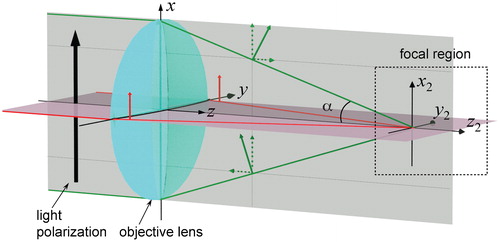
In order to study the influence of the input light polarization on the intensity and polarization distributions at the focusing region of an OL, we assume that the incident beam is linearly polarized along the x axis (black arrow), as illustrated in Fig. 1. The diffracted light rays located in the (x₂z₂) and (y₂z₂) planes show different projected polarization components. Indeed, light rays located in the (y₂z₂) plane (red arrows) keep their original polarization states (x linear polarization component only), while for the light rays located in the (x₂z₂) plane, a second longitudinal (z) component appears. The longitudinal components are opposite in sign (π-phase shift) for rays located in the positive half plane (x₂>0) and those located in the negative half plane (x₂<0). This leads to a complex interference effect of all light rays, resulting in different intensity and polarization distributions at the focusing region. Furthermore, the strength of this longitudinal component becomes important when the α angle increases. Therefore, a high NA OL (large α angle) induces a non-negligible longitudinal component.

Figure 1. Schematic diagram illustrating focusing effect and polarization dependence of linearly polarized light beam focused by high numerical aperture objective lens (OL): green and red arrows illustrate polarization states of light rays, propagating in (xz) and (yz) planes respectively after passing through OL

Figure 2 shows the numerical calculation of the intensity and polarization distributions of an x linearly polarized beam (p_x = 1, p_y = 0, p_z = 0) under a tight focusing condition [NA = 1.4 (α≈67.5°), n = 1.515]. As shown in Fig. 2d (total intensity distribution), the focusing spot possesses an elongated shape along the input polarization direction. This confirms the above prediction that, for tight focusing, the input polarization influences the focusing shape. The asymmetric focusing spot comes from the fact that behind the fundamental x component (Fig. 2a), which has almost a symmetric shape with around 85.5% of the total intensity, there is a contribution of the z component (Fig. 2c), which is about 14% of total intensity in this case. For tight focusing, the z component has a doughnut shape because of the constructive and destructive interference of different light rays in the focal region. Indeed, as mentioned previously, two symmetric rays, one from the positive half plane (x₂>0) and other from negative half plane (x₂<0), have the same longitudinal component values with a π-phase difference, resulting in a destructive interferences for all the points located on the z axis. The longitudinal components of other rays (phase difference = π) are different and will be added up resulting in non-null intensity, distributed symmetrically around the z axis and represented by a doughnut. We note that the numerical result also shows the existence of another lateral component (Fig. 2b), but it contributes only 0.5% of the total intensity, a negligible contribution to the focusing spot shape.

Figure 2. Numerical calculation of a–d intensity and e, f polarization distributions in focal region of high NA OL (NA = 1.4, n = 1.515): input light beam is linearly polarized along x axis, as shown in left; intensity distributions in (x₂y₂) plane are calculated for different components: a

, b

, c

and d

; polarization distributions are calculated for e (x₂y₂) plane and f (x₂z₂) plane respectively; small lines and their directions indicate polarization directions of light in focal region and their lengths are proportional to field strength; intensities of all images are normalized to total intensity

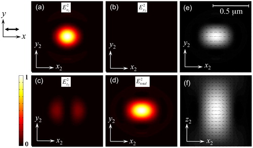
The polarization distribution in the (x₂y₂) plane (Fig. 2e) further illustrates that the component plays a dominant role. However, this polarization does not remain the same for different (x₂y₂) plane in the focusing region. Figure 2f shows the polarization distribution in the (x₂z₂) plane, in which we can see that the polarization varies slightly at different z₂ positions [different (x₂y₂) planes]. This is again a consequence of the longitudinal component created by the tight focusing effect.

In contrast to a x linear polarized incident beam, the circularly polarized light induces a symmetric intensity distribution in the (x₂y₂) plane as shown in Fig. 3. It is a very popular image obtained by an optical microscope or an optical confocal laser scanning system, since the light source used in most systems is incoherent (non-polarized) or coherent with a circular polarization. This symmetry can be explained by the fact that the x and y components show equivalent polarizations strengths in the case of circular polarization (p_x = 1/2^1/2, p_y = i/2^1/2, p_z = 0). Hence, there are two equivalent lateral components, (Fig. 3a) and (Fig. 3b), with the same portion of 46% of the total intensity. In this case, the longitudinal component also appears for all diffracted rays, symmetrically around the optical axis of the OL, and induces an intensity contribution of around 8% of the total intensity, represented by a doughnut spot in focal region (Fig. 3c).

Figure 3. Numerical calculation of a–d intensity and e, f polarization distributions in focal region of high NA OL (NA = 1.4, n = 1.515): input light beam is circularly polarized, as shown in left; intensity distributions in (x₂y₂) plane are calculated for different components: a

, b

, c

and d

; polarization distributions are calculated for both e (x₂y₂) plane and f (x₂z₂) plane respectively; small lines and their directions indicate polarization directions of light in focal region and their lengths are proportional to field strength; intensities of all images are normalized to total intensity

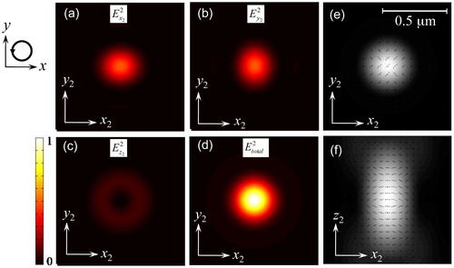
Concerning the polarization distribution at the focusing region, we obtain a circular polarization distribution in the focal plane (Fig. 3e). However, similar to the case of linear polarization, this polarization varies with different z₂ positions [different (x₂y₂) planes]. The polarization distribution, caused by either linear or circular input polarization, is quite important for the applications in which the control of light polarization and the optical dipoles of molecules are necessary.

In summary, in a tight focusing system, the intensity and polarization distributions depend strongly on the polarization of the input light field. In the next section, we introduce an experiment to characterize the shape of the focusing spot (intensity distribution) of a high NA OL using different input polarizations.

Experimental demonstration of influence of input beam polarization on focusing spot shape

The experimental demonstration of the influence of the input light polarization on the focusing spot shape is carried out by a home made confocal microscope. The optical system is mounted on an active isolation optical table to prevent the system from external movement caused from environment. The schematic representation of the optical set-up is shown in Fig. 4. A large and uniform laser beam emitting at 532 nm wavelength is employed as an excitation light source. The laser beam is tightly focused into the sample by an oil-immersion OL with NA = 1.4. The sample is a glass thin film covered with gold nanoparticles (diameter of 50 nm), each of which being assumed to be a point-like object. The gold nanoparticles are sandwiched in between two SU-8 photoresist thin films to avoid aberration effects. The sample is mounted on a three-dimensional piezoelectric translation, which allows positioning gold nanoparticles with a resolution of 0.2 nm. The laser beam at 532 nm excites gold nanoparticles, which then emit a fluorescence light at λ>532 nm. We assume that the gold nanoparticles have a spherical shape, perfectly isotropic and thus insensitive to the excitation polarization. Therefore, excitation and emission are equivalent for any polarization at any direction. The emitted photons are collected by the same OL and are sent back to a set of focusing/collimating lenses, pinhole (100 μm in diameter), filter (long pass filter with a cutoff wavelength of 535 nm) and avalanche photodiode detector, as shown in Fig. 4. By scanning the sample in three-dimension, the intensity distribution of focusing spot is then reconstructed.

Figure 4. Schematic representation of experimental set-up used to evidence influence of input beam polarization on shape of tightly focused spot (PZT: piezoelectric translator; OL: oil immersion microscope objective, with NA = 1.4, ×100; BS: beam splitter; λ/2: half-wave plate; λ/4: quarter-wave plate; L1–L3: lenses; PH: pinhole; F: 580 nm long pass filter; APD: silicon avalanche photodiode)

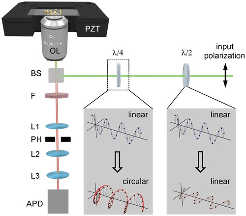
In this set-up, in order to characterize the influence of the excitation polarization, we have used some phase plates. Initially, the laser beam is linearly polarized along the x axis. Its direction (linear polarization) is then controlled by rotating the half-wave plate (λ/2), as depicted in the grey part of Fig. 4. To produce a circular polarization, a quarter-wave plate (λ/4) is introduced behind the λ/2, the incident linear polarization (after λ/2) being oriented at 45° with respect to the neutral (fast or slow) axis of the λ/4. Depending on the aim of the work, either λ/2 or both λ/2 and λ/4 plates can be used.

First, in absence of the λ/4 plate, we scanned laterally the focusing spot with a linearly polarized incident beam and measured the fluorescence image of a single gold nanoparticle. Figure 5a shows that the shape of focusing spot is elongated in the same direction as that of the input beam polarization (here along the x direction). By changing the polarization direction, we observed that the asymmetric distribution property changed accordingly. Figure 5b and c shows fluorescence images of the same gold nanoparticle excited with a linear beam polarization at 45 and at 110° respectively. The rotation of the focusing spot shape confirms that its asymmetric property is due to the polarization of input beam, which is consistent with the theoretical prediction presented in the section on ‘Theoretical calculation of intensity and polarization distributions of tightly focused beam’. Furthermore, by introducing the λ/4 plate, with an appropriate orientation with respect to the direction of the linear polarization to result in a circular polarization, we obtained a fluorescence image with a perfectly symmetric focusing shape, as shown in Fig. 5d. This result confirms also the theoretical prediction shown in Fig. 3a.

Figure 5. Experimental observation of dependence of focusing spot shape on polarization of incident beam [input beam polarization (green circle) of each image: linear polarization at a 0°, b at 45°, c at 110° and d circular polarization respectively]

To quantitatively evaluate the shape and size of the focusing spot obtained with different polarizations, we extracted the data from Fig. 5 for two orthogonal axes, according to the minimal and maximal sizes of the focusing spot. Figure 6 shows a comparison between theoretical and experimental results. In the case of a x linear polarized incident beam (Fig. 6a), the calculated full width at half maximum (FWHM) of the total intensity distribution along the y axis (FWHM = 240 nm) is only 70.5% of the one along x axis (FWHM = 340 nm). This ratio is in good agreement with the numerical calculation result (71.4%) shown in Fig. 6b. In the case of circular polarization, the focusing spot is symmetric and the spot has the same size (FWHM = 280 nm) along both axes, as shown in Fig. 6d, which is also in agreement with the theoretical curves shown in Fig. 6c. Nevertheless, as compared to the simulation results, the focusing spot measured experimentally has a larger size, of about 40 nm for any axis and for both polarizations. This difference can be explained by the fact that, in practice, we have used a gold nanosphere as a probe bead with a diameter of 50 nm (it still cannot be an ideal point-like object). Thus, the experimental intensity profile is a convolution size of an ideal (theoretical) focusing spot and the gold nanosphere size. The experimental data can be further optimized by applying the image deconvolution method²⁰ to fit the theoretical calculation. However, it is not necessary in our case, since the polarization dependence of the focusing spot is clearly evidenced.

Figure 6. Comparison of a, c experimental and b, d theoretical results of focusing spot profile, along x₂ axis (red color) and y₂ axis (blue color) for a, b linear and c, d circular polarizations: experimental curves are extracted from images plotted in Fig. 5a and d; theoretical curves are derived from numerical calculation shown in Figs. 2d and 3d respectively; size (FWHM, full width at half maximum) of focusing spot, calculated along each axis, is indicated in each figure

Conclusion

In conclusion, we have demonstrated that, under tight focusing condition, the focusing spot shape depends strongly on the polarization of the input light beam. Using a light beam with circular polarization, we obtained a symmetric focusing spot, with a transverse size close to the diffraction limit. However, with a linearly polarized incident light beam, the focusing spot elongated along the direction of the light polarization, resulting in an asymmetric submicrometer focusing spot. This polarization dependence of the focusing spot is numerically explained by using a vectorial Debye theory, and experimentally demonstrated by mapping the fluorescence of single gold nanoparticles using a confocal system with a high NA OL. Besides, the theoretical calculation also provides information about the polarization distribution at the focusing region, which depends on the polarization of input light beam. The understanding of the intensity and polarization behaviors of the focusing spot of a high NA OL on the input beam polarization is of great importance for many applications, such as high resolution imaging, nanofabrication, optical manipulation, etc.

Conflicts of interest

The authors declare that there are no conflicts of interest.

References

- T. Wilson: ‘Confocal microscopy’; 1990, London, Academic Press.
- A. Ashkin, J. M. Dziedzic and T. Yamane: Nature, 1987, 330, 769–771.
- M. Deubel, M. von Freymann, G. Wegener, S. Pereira, K. Busch and C. M. Soukoulis: Nat. Mater., 2004, 3, 444–447.
- M. T. Do, T. T. N. Nguyen, Q. Li, H. Benisty, I. Ledoux-Rak and N. D. Lai: Opt. Express, 2013, 21, (18), 20964–20973.
- M. Farsari and B. N. Chichkov: Nat. Photon., 2009, 3, (8), 450.
- D. A. Parthenopoulos and P. M. Rentzepis: Science, 1989, 245, (4920), 843–845.
- K. Venkatakrishnan, B. Tan, P. Stanley and N. R. Sivakumar: J. Appl. Phys., 2002, 92, (3), 1604–1607.
- B. Richards and E. Wolf: Proc. R. Soc. Lond. Ser. A, 1959, 253A, (1274), 358–379.
- H. Kang, B. Jia and M. Gu: Opt. Express, 2010, 18, (10), 10813–10821.
- L. Egil Helseth: Opt. Commun., 2002, 212, (4), 343–352.
- D. Ganic, X. Gan and M. Gu: Opt. Express, 2003, 11, (21), 2747–2752.
- M. J. Nasse and J. C. Woehl: J. Opt. Soc. Am. A, 2010, 27A, (2), 295–302.
- X. Hao, C. Kuang, T. Wang and X. Liu: J. Opt., 2010, 12, (11), 115707.
- S. N. Khonina and I. Golub: Opt. Lett., 2011, 36, (3), 352–354.
- G. P. Karman, A. van Duijl, M. W. Beijersbergen and J. P. Woerdman: Appl. Opt., 1997, 36, (31), 8091–8095.
- S. K. Rhodes, K. A. Nugent and A Roberts: J. Opt. Soc. Am. A, 2002, 19A, (8), 1689–1693.
- R. Dorn, S. Quabis and G. Leuchs: J. Mod. Opt., 2003, 50, (12), 1917–1926.
- C. Huber, S. Orlov, P. Banzer and G. Leuchs: Opt. Express, 2013, 21, (21), 25069–25076.
- A. van de Nes, L. Billy, S. Pereira and J. Braat: Opt. Express, 2004, 12, (7), 1281–1293.
- B. Simon and O. Haeberlé: J. Eur. Opt. Soc., 2006, 1, 06028.