Differences in Surface Roughness, Energy, and CO₂ Fluxes in Two Moist Tundra Vegetation Types, Kuparuk Watershed, Alaska, U.S.A

Abstract

Roughly 70% of the tundra north of the Brooks Range, Alaska, can be classified as moist nonacidic (39%) and moist acidic tundra (31%). We investigated the differences in energy partitioning and carbon balance among these two important landscape types. Despite structural differences in plant growth forms, moss cover, and soil pH, the sensible and latent heat fluxes were quite similar. However, aerodynamic properties (i.e. roughness length), ground heat flux, and CO₂ flux were significantly different: aerodynamic roughness of moist acidic tundra was 2.1 times higher than, and ground heat flux was 36% lower than the values obtained from moist nonacidic tundra. Daily carbon balance showed 26% more net CO₂ uptake (with 34% greater ecosystem respiration and 30% greater gross primary production) in moist acidic tundra. The greater respiration rate in moist acidic tundra was explained by differences in surface soil temperatures, whereas the rate of gross primary production was only half of what was expected from observed differences in leaf area index. These differences suggest that understanding the controls of CO₂ exchange in nonacidic moist tundra vegetation will be critical for determining the carbon budget of the Low Arctic region.

Introduction

The Arctic region is expected to experience the greatest changes in annual mean temperature according to the Intergovernmental Panel on Climate Change (IPCC) scenarios (Cubasch et al., 2001). Tundra vegetation types which are adapted to very short growing seasons of only few months and are expected to react very sensitive to such climatic changes. Any response of the local vegetation will also feed back to the climate system (e.g., Eugster et al., 2000). The knowledge of energy and carbon fluxes is essential for understanding feedbacks of local vegetation to climate. Energy partitioning at the soil-vegetation-atmosphere interface is the most important biophysical process in global-scale circulation models (GCM). Inaccurate representation of this process for important vegetation types could lead to large errors in the ability of GCMs to represent actual climate, as well as to model climate-change scenarios. Our focus in this paper is on regional and thus—in GCM terminology—subgrid scale variation in surface fluxes (e.g., McFadden et al., 1998). At present, most dynamical atmospheric models parametrize arctic landscapes with only one surface type. Yet abundant field data and remote-sensing observations show large differences in vegetation structure and primary productivity among different tundra landscape types. To use a single surface type for tundra in a mesoscale model or GCM might be as inappropriate as choosing a single type of forest to represent temperate and tropical forests, coniferous and deciduous forest at the same time. For example, a regional climate model representing northern Alaska yielded a 3.5°C warmer summer (June–August) temperature over shrub than moist tundra (Chapin et al., 2000). In this paper we present results of direct comparisons between the two most common types of upland tussock tundra, moist nonacidic and moist acidic tundra, which cover 38.9 and 30.8%, respectively, of the Kuparuk watershed, Alaska (Auerbach and Walker, pers. comm.; Muller et al., 1998, 1999). Until the mid-1990s, research focused almost exclusively on acidic tundra which was believed to be representative of moist tundra in general. Walker and Everett (1991) were the first to describe the importance of nonacidic tundra, and more recent studies (Walker et al., 1998; Gough et al., 2000) confirm the significant role of soil pH in tundra ecosystems. The present experiment was designed as a first assessment of the quantitative differences in biosphere-atmosphere exchange fluxes of nonacidic tundra in comparison with acidic tundra.

Sites and Methods

SITE SELECTION

Moist acidic and moist nonacidic tundra look very similar on the ground but have distinct spectral characteristics in satellite images (Walker and Everett, 1991; Walker et al., 1998) and species composition. Species richness is generally higher in nonacidic tundra (Gough et al., 2000). Nonacidic tundra has a soil pH > 6.5, while acidic tundra has a pH < 5.5 (Walker et al., 1998). Recent loess deposits prevent the nonacidic tundra from becoming more acidic in soil pH during the landscape aging process (Walker and Everett, 1991). Moist acidic tundra features dwarf shrubs with dwarf birch (Betula nana) (plant names are taken from Hultén [1968]) and willows (Salix phlebophylla being the most abundant) partially covering the ground, with a mean leaf area index (LAI) of 0.84, whereas moist nonacidic tundra is almost shrubless with an LAI of 0.50 (Table 1). In moist acidic tundra 79% of the ground surface is covered with moss (dominated by Sphagnum peat mosses) whereas moss cover is 65% in moist nonacidic tundra (nonpeat mosses) (Table 1). In the following, the moist acidic tundra site is designated as MAT (69°24.06′N, 148°48.34′E, 360 m a.s.l.) and the moist nonacidic tundra site as MNT (69°26.46′N, 148°40.22′E, 269 m a.s.l.). At that latitude, continuous permafrost restricts rooting depth of plants to a thaw layer typically not more than 30 to 60 cm in depth. The two sites, located 7 km apart, were chosen to be as similar as possible in terms of mesotopography (rolling hills, on crest of smooth hills) and drainage. Patches of homogeneous vegetation were selected that are representative of the MAT and MNT types as classified in a satellite-derived vegetation map of the region (Muller et al., 1998, 1999), which together comprise 70% of the tundra in northern Alaska. A comparative approach was used (Eugster et al., 1997), measuring eddy covariance fluxes of energy, water vapor, and CO₂ with two towers that were operating simultaneously at the MAT and MNT sites for 9 d (21 to 29 June 1995) during the Arctic System Science (ARCSS) Flux Study. This period was 3.1°C cooler than normal (Table 2). However, the preceding 30 d were 0.2°C warmer than normal, which suggests that the vegetation status was very close to average at the time of our measurements. Precipitation of the previous 30 d was twice the normal amount, while during our measurements the precipitation sum was only 7.5% above normal. The excess precipitation prior to our measurements should not have led to a significant difference in vegetation status since this type of tundra is moist tundra. The two sites are labeled 95-4 (MAT) and 95-3 (MNT) in the ARCSS data base. Data are archived and available from the National Snow and Ice Data Center, Boulder, Colorado (Chapin et al., 2002).

INSTRUMENTATION AND DATA AQUISITION

At each site a mobile tower consisting of a foldable tripod 3 m tall (Met One Instruments, Grants Pass, OR, U.S.A., model 905) was installed with a sonic anemometer (Applied Technologies Inc., Boulder, CO, U.S.A., models SWS-211/3V and SAT-211/3Vx), a combined H₂O/ CO₂ closed-path IRGA (infrared gas analyzer; LI-COR, Lincoln, NB, U.S.A., model 6262), radiation sensors (Fritschen-type net-radiation from Radiation and Energy Balance Systems [REBS], Seattle, WA, U.S.A.; global radiation and quantum sensor from LI-COR), a combined temperature/humidity sensor (Vaisala-type; Campbell Scientific, Logan, UT, U.S.A., model HMP35C), and four sets of soil heat flux plates and platinum resistance soil temperature sensors (REBS) that were placed in major microsite types (see Table 3). The gas-sampling tube (3.2 mm inner diameter, approximately 2 m long) was placed 15 cm from the center of the sonic anemometer transducer array, perpendicular to the axis of the transducer pair closest to the inlet to minimize both the effect on the turbulence measurements and the effect of the separation between wind measurements and trace gas concentration measurements. Air was drawn through the IRGA at 8–9 L min⁻¹ by a 12 V DC diaphragm vacuum pressure pump (Barnant Company, Barrington, IL, U.S.A., model 400-1903) with a flowmeter and sufficient vacuum hose (1 m) between it and the IRGA to reduce the pulsation of the diaphragm. Data from the radiometers and soil sensors were recorded on a data logger (Campbell Scientific, model 21X), and the signals from each gas analyzer were read by an analog-to-digital board at 12-bit resolution (the resolution of the LI-COR 6262 analog output) and saved to the same portable computer that captured the output from the sonic anemometer. A computer program synchronized the signals and computed fluxes in real time. Eddy covariance instruments and net radiometers were mounted at 1.80 m (MAT) and 1.79 m (MNT) above the surface. All 20 Hz raw data were recorded for later processing. Raw data were screened for spikes, and H₂O and CO₂ fluxes were calibrated for high frequency and damping losses according to the procedure described in Eugster and Senn (1995). Radiation instruments were compared at Happy Valley on 17–19 June 1995 (prior to field deployment; data not shown). The complete flux measurement systems used at the two sites were tested in a side-by-side intercomparison at a nearby site in 1996 (Eugster et al., 1997). The relative accuracy of turbulent flux measurements was found to be better than 15%, which is good for currently available equipment (Eugster et al., 1997). To make the energy and carbon dioxide flux measurements from both sites comparable, the subset of half-hourly values which were measured at both sites simultaneously within the total measurement period was selected. Then, using the set of simultaneous measurements, average diurnal cycles with hourly resolution were computed for each site. Data are presented with the hourly values centered at the hour, covering the interval of the full hour ± 30 min.

VEGETATION AND SOIL MEASUREMENTS

Because the eddy covariance technique provides measurements of only net fluxes (net ecosystem exchange, NEE), ecosystem respiration (ER) was estimated from the NEE values measured when the sun was lowest. Because it never gets completely dark at this time of year we selected all records from between 0030 and 0430 ADT with an observed photosynthetic photon flux density PPFD <50 μmol m⁻² s⁻¹ and determined the net CO₂ flux for 0 μmol m⁻² s⁻¹ light using a linear regression,

This approach is similar to the one presented by Gilmanov et al. (2003), but it is expected to be less sensitive to uncertainties in statistical fits to small datasets. Nine days of measurements have some limitations compared to long-term flux measurements when it comes to time-resolved estimation of ER (Fig. 1). Gross primary production (GPP) was then obtained by subtracting ecosystem respiration from NEE (note that we use positive signs for CO₂ fluxes directed away from the surface and toward the atmosphere). At each site tussock height was estimated from the residuals of a second-order polynomial fitted to three transects of microtopographical elevation measurements. Two transects were 100 m long, and one was 141 m long, corresponding to the two perpendicular centerlines and one diagonal of a 100 × 100 m square with the flux tower located in its center. Sampling interval was 5 m (N = 71 points). Leaf area index (LAI) was measured with a LI-COR LAI-2000 plant canopy analyzer along the same transects described above. Sampling points were identical with the microtopographical measurements. The measurements from the plant canopy analyzer were then corrected for litter and stem shading. This was done by applying conversion factors that were derived from the comparison of optical LAI measurements with the LAI determined by harvesting a 40 × 40 cm² area. In the case of stems from dwarf shrubs, the optically measured area index was 1.8 times the projected stem area index (Eugster et al., unpublished data). At each site soil temperature and ground heat flux data were measured in four representative microsites (Table 3), and soil moisture was determined gravimetrically at the end of the measuring period. The selection of microsites was done visually based on the spatial variation of microtopography and the expected differences in soil and surface properties. Volumetric moisture contents were 19.8, 21.6, 24.0, and 38.4% for the four MNT microsites, and 20.3, 24.7, 25.1, and 29.5% for MAT. Ground heat flux was measured with heat flux plates at 5 cm depth below the surface, corrected for the heat storage term between the surface and the heat flux plates which was calculated from measured temporal changes in soil temperature, the proportional volumetric content of water, mineral soil, and organic matter. Diurnal variations of soil moisture were recorded continuously with an electronic probe (Hydra, Vitel Inc., Chantilly, VA 22021, U.S.A.) at each site. There was no trend in average soil moisture over the 9 d of our measurements, and thus using a constant soil moisture in the computation of soil heat capacity is not expected to lead to a significant bias in reported ground heat fluxes for the whole period. The fluffy peat soils make it difficult to define the ground surface reference for measurements. In this paper we adopted the convention to use the visible surface as the ground surface reference, which can be the surface of a dense moss mat or the mineral soil surface of frost boils, depending on microhabitat. Thus, ground heat fluxes reported here refer to this surface, which is also the relevant surface for determining sensible and latent heat flux, although light might penetrate a few centimeters farther down into the nonturbulent volume of dense moss mats.

Results and Discussion

The largest differences between MAT and MNT were found in aerodynamic roughness length z ₀ (and thus momentum fluxes), ground heat flux (G), and CO₂ flux, while turbulent sensible heat (H) and latent heat (LE) fluxes were rather similar on average.

AERODYNAMIC ROUGHNESS

Although the mesotopography (size of ridge and valley systems) was similar at both sites, local microtopography (tussocks and intertussock space) was different. Roughness lengths were calculated from eddy covariance momentum flux measurements u w using the diabatic wind profile equation (e.g., Panofsky and Dutton, 1984) solved for z ₀, with z measurement height above displacement height, u mean horizontal wind speed, k the von Kàrmàn constant (0.40), z/L the Monin-Obukhov stability parameter (Monin and Obukhov 1954), and Ψ_m(z/L) the stability correction term (see Paulson [1970] for additional details). Only data collected at near-neutral stability (z/L was in the range −0.1 to +0.1) with momentum flux directed towards the surface (i.e., u′w′ < 0) were used to determine z ₀ since other processes than mechanical turbulence may be governing the wind profile under very stable and very unstable conditions. Overall, 61 to 69% of the flux measurements satisfied these criteria. Roughness lengths at the MAT site were larger than at the MNT site by a factor of 2.1 (Table 1). Color near-infrared aerial photographs of both sites indicate that the vegetation is slightly less homogeneous at the MNT site than at the MAT site. The greater z ₀ at the MAT site reflects both a greater abundance of shrubs, which add aerodynamic roughness, taller tussocks, which produce the uneven topography characteristic of tussock tundra, and greater LAI (Table 1). Although the differences in aerodynamic roughness are large, turbulent mixing of the atmosphere above the two ecosystems does not generally appear to be a limiting factor for energy exchange and CO₂ fluxes. Only 7.3% (MAT) to 8.3% (MNT) of all measurements were performed during stable conditions with z/L > 0.1. The lack of a dark night (no sunset was observed during the time period of our measurements) kept turbulent mixing over the tundra active 24 h a day. Roughness lengths were large when compared with the canopy height (Table 1). Over flat surfaces, the generally adopted rule of thumb for estimating z ₀ is 15% of canopy height for various crops and grasslands (Plate, 1971). Our measurements, however, show almost an order of magnitude greater z ₀. Since the effective roughness of a surface is always a combination of vegetation elements and microtopographical variation, our measurements document the importance of small-scale surface roughness structures such as the tussocks and individual dwarf shrubs that add significantly to the overall roughness of the landscape. Since tussock height is greater than the canopy height of the plants themselves, it could be argued that the tussocks are the primary roughness elements of arctic tundra landscapes. As compared with textbook values (e.g., Panofsky and Dutton, 1984), MAT and MNT roughness lengths correspond to farmland values representative of long grass or crops (similar to MAT–z ₀) or uncut grass (MNT–z ₀), respectively.

ENERGY FLUXES

Despite the large differences in roughness lengths of the two vegetation types, the differences in sensible and latent heat fluxes between the two sites were not significant. Roughness lengths govern turbulent mixing above the land surface and potentially could lead to significant site-specific conditions for sensible and latent heat transfer from the surface to the atmosphere, especially at low wind speeds. It was therefore surprising to find that roughness lengths (Table 1) and thus momentum fluxes differed strongly between MAT and MNT according to their differences in vegetation structure, but not so sensible and latent heat flux (Fig. 2). From this we conclude that turbulent mixing above tundra is not a limiting factor for vegetation-atmosphere exchange processes, despite the frequently occurring low wind speeds which are also easily observed via the high abundance of mosquitoes in the air. The two sites experienced similar net radiation (R_n, Fig. 2), except for mid-day when local cloudiness was slightly different (note that local noon is 1400 ADT) as indicated by high mid-day variability in net radiation. Site differences in R_n were associated with parallel differences in H while the minor differences in LE occurred 3 h later. However, these differences do not appear to be significant given the high day-to-day variations in R_n, H, and LE, as expressed by the vertical bars in Figure 2. The regression slopes of MAT data against MNT data were not significant at the 95% confidence level for R_n, H, and LE, respectively. To account for serial correlation in the data (lag 1 autocorrelation coefficients ranged between 0.86 for F_CO2 and 0.98 for G) the confidence intervals were enlarged via the variance inflation factor according to Wilks (1995). Some uncertainty remains in these comparisons due to differences in energy budget closure at the two sites. While both flux measurement systems yielded similar energy budget closures in our intercomparison reported by Eugster et al. (1997), we observed closures (H + LE)/(R_n − G) of 87% at the MAT and 74% at the MNT site, values which are in the range observed at many places in the world (Wilson et al., 2002). Ground heat flux differed significantly between sites (by more than the relative measurement error determined by a direct intercomparison [Eugster et al., 1997]). At the MAT site, G was only 64% of that at the MNT site (Table 4). The slope of the regression of G at MAT against G at MNT was also less than 1.0, which was significant at the 95% confidence level. There was an inverse relationship between G and the soil temperatures that were measured close to the surface. At the MAT site less heat was conducted to the lower soil layers, which was in agreement with the reduced thaw depth and greater coverage of insulating mosses (Table 1) which leads to higher near-surface soil temperatures compared to MNT. This is in contrast to the conditions that would be expected with purely mineral soils where greater surface-soil temperatures should lead to greater G. This indicates the relevance of the insulating moss layer in this environment as an interfacial layer between the atmosphere and the soil.

CARBON DIOXIDE FLUXES

The key question with respect to ecosystem respiration is whether higher G implies higher or lower ground surface and soil temperatures. Vourlitis et al. (2000) showed for a moist-tussock tundra versus wet-sedge tundra comparison that moisture (in their study represented by depth to water table) explained more of the variation in ecosystem respiration than did temperature. While their moist-tussock tundra corresponded to the MAT ecosystem type we studied, their wet-sedge tundra was not similar to the MNT ecosystem described here. Wet-sedge tundra has a higher water table (wetland aspect), whereas MNT has a similar upland morphology as does MAT. Therefore, differences in depth to water table are not expected to control differences in surface energy exchange between the sites we studied. In both MAT and MNT vegetation types, the highest moisture contents coincided with the lowest temperatures. In MAT there was considerable variation in surface-soil temperatures among the microsites, while surface-soil temperatures at the MNT microsites were all within 3°C of each other. The opposite pattern was shown by G: surface-soil temperatures were generally lower in MNT where ground heat flux was larger than in MAT (Fig. 2). Both sites showed a consistent, inverse relationship between thermal conductivity and heat capacity: high temperatures implied low G and vice versa. However, differences in species composition, especially mosses, appeared far more important than soil moisture content. Mosses act as insulators on hummocks where their surface dries out quickly during sunny days, leading to higher surface temperature but lower G. Among the investigated environmental factors, Gough et al. (2000) found soil pH to be the dominant factor that explains variations in species richness. This confirms earlier findings (Walker et al., 1998) that landscape age exhibits a strong control over vegetation composition via soil pH. The findings by Gough et al. (2000) also suggest that differences in energy or CO₂ exchange between the arctic tundra ecosystems and the atmosphere are strongly controlled by the vegetation which acts as the interface between the processes in the soil (active layer) and the turbulent mixing in the atmospheric boundary layer. Site differences caused large differences in carbon fluxes (GPP, ER, and NEE; Table 5). Thus, MAT, the site with greater shrub biomass and warmer soils, had higher rates of both gross photosynthesis (GPP) and ecosystem respiration (ER) than did MNT (Table 5). Relative differences in GPP were of similar magnitude (+30% in MAT) as ER (+34% in MAT, see below), although the relative differences in leaf area index were much larger (68%, Table 1). The net effect of these differences in carbon gain and loss was a 26% higher net carbon gain during the measurement period in MAT than in MNT. The greatest relative differences were found in ER. Owing to the fact that respiration of tussock-tundra soils shows little response to temperatures below 10°C (Schimel et al. [1996]; but see also Mikan et al. [2002] for the effect of increased respiration rates in frozen soils), the differences in respiration are attributed to different soil organic matter content and quality and moisture conditions, leading to a 34% higher respiration rate in MAT in comparison with MNT (Table 5). Although soil temperatures differed significantly between MAT and MNT (Table 1) we did not find a generally valid relation between ER and soil temperature (McFadden et al., 2003), suggesting that other site-specific factors than soil temperature must be responsible for differences in ER. Vourlitis et al. (2000) report 14% greater ER (1943 mg C m⁻² d⁻¹) from their MAT site compared to wet tundra during a 92-d long measurement period between 1 June and 31 August 1995 (site location 69°08.54′N, 148°50.47′W). Over this period, the net carbon uptake was −600 mg C m⁻² d⁻¹, which is only 53% of the value we measured at our MAT site (Table 5) during the peak of the same growing season. Another season-long measurement at a MAT site from 1995 (near Happy Valley, 69°07′N, 148°50′W) yielded a daily average net carbon gain of −510 mg C m⁻² d⁻¹ during a 100-d measuring period (Harazono et al., 1996). This is not surprising, because soil temperatures lag daily insolation by roughly 1.5 mo in this region of continuous permafrost (Eugster et al., 1997). For this reason, the temperature dependent rate of ER peaks later in the growing season than does GPP. The present study reflects conditions in the first half of the growing season. Seasonal estimates made for 1995 and 1996 based on a combination of other mobile and permanent tower flux measurements also yielded the same qualitative difference in MAT and MNT CO₂ exchange. The MNT sites (27.6 and 3.3 g C m⁻² season⁻¹ in 1995 and 1996, respectively), however, responded more strongly also to differences in summer climate conditions than did the MAT sites (55.2 and 52.5 g C m⁻² season⁻¹, respectively) (data from Walker et al., 1998). Field experiments in moist and dry tundra ecosystems show that responses of CO₂ fluxes to environmental manipulations are most pronounced during the short summer (Welker et al., 2000), although carbon losses continue during winter (Jones et al., 1999). The growing-season comparison reported here does not provide the information to construct annual carbon budgets for MAT and MNT. However, comparison of our short-term measurements with season-long measurements at comparable MAT sites documents the value of mobile (paired) towers also for assessing regional variation in carbon fluxes among ecosystem types. Although seasonal sums of NEE differ from short-term measurements, the relative magnitudes of NEE, ER, and GPP measured over short (10 d) periods provide essential information for (1) deciding where to place long-term measuring towers in order to derive seasonal spatial patterns; (2) interpreting satellite-derived vegetation data (McMichael et al., 1999); (3) numerical modeling (e.g., Williams et al., 2000); or (4) establishing functional relationships between environmental drivers and CO₂ fluxes (McFadden et al., 2003).

Conclusions

Significant differences were found between the two most widespread vegetation types of arctic Alaska in aerodynamic roughness length, ground heat flux, surface-soil temperature, and carbon flux. The differences in ground heat flux were inversely related to differences in surface-soil temperature, suggesting that mosses are particularly important for understanding surface energy partitioning in tundra vegetation. Mosses control surface energy partitioning in arctic tundra in two ways. When wet, they cool the surface by evaporating water and at the same time increase thermal conductivity, which increases ground heat flux. When dry, mosses insulate the surface, leading to rather high surface temperatures, while decreasing the ground heat flux. These differences in the thermal regimes of the ground surface between MAT and MNT had important feedbacks on carbon fluxes. Ecosystem respiration was 34% greater in the acidic tundra in agreement with the significantly higher surface-soil temperatures. This, in combination with higher gross primary production in MAT, led to a difference in daily net carbon uptake of 26% between the two vegetation types. The small site differences in sensible and latent heat fluxes were not significant, suggesting that structurally similar tundra vegetation types have similar turbulent energy fluxes. The comparison of our short-term (10 d) flux measurements from mobile towers with season-long measurements from permanent towers indicates that the relative difference between directly compared ecosystems are representative of what could be found with season-long measurements, although the magnitudes of the seasonal carbon budgets depend on the timing during the growing season when the mobile towers are deployed. These differences suggest that understanding the controls on CO₂ exchange in nonacidic moist tundra vegetation will be critical for determining the carbon budget of the Low Arctic region.

FIGURE 1. Light response of moist acidic (MAT) and moist nonacidic (MNT) tundra. Ecosystem respiration (thin horizontal lines) is determined from the intercept of a linear regression (thick lines) to the data at PPFD <50 μmol m⁻² s⁻¹. Data recorded when the wind direction was from the sector 330–340° (MAT) or 300–305° (MNT) were excluded. The regressions (best fit ± standard error of fit) for MAT and MNT are F_c = (0.020 ± 0.003) − (0.00038 ± 0.00009) PPFD (r ² = 0.46), and F_c = (0.015 ± 0.002) − (0.00029 ± 0.00006) PPFD (r ² = 0.52), respectively

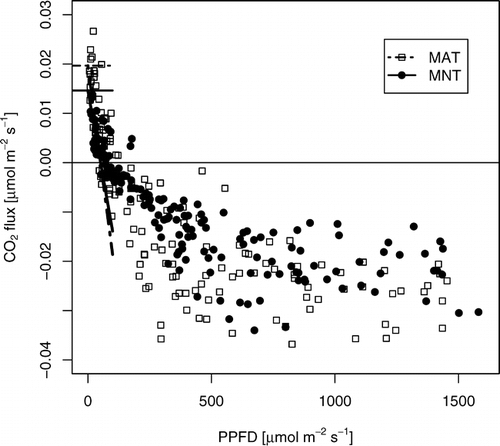
FIGURE 2. Comparison of average diurnal cycles of energy (Rn, G, H, LE) and CO₂ fluxes, and surface-soil temperatures (Tsoil). Measurements were obtained during a 9-d period (21–29 June 1995). Open circles, solid lines: moist nonacidic tundra; filled squares, dashed lines: moist acidic tundra. Alaskan daylight savings time (ADT) is UTC−8 h. Only data records measured simultaneously at both sites were considered. Vertical bars denote ± 1 standard deviation

TABLE 1 Comparison of properties of moist acidic (MAT; Site 95-4) and moist nonacidic tundra (MNT; Site 95-3) types, average ± standard error

TABLE 2 Characteristics of air temperature measured at the Toolik Lake LTER site (68°38′N, 149°36′W, 760 m a.s.l.) during the period of flux measurements and the preceeding month with respect to the station's 16-yr mean, 1988–2003.^a

TABLE 3 Characteristics of the microhabitats where soil heat flux plates were inserted at 5 cm depth and soil temperatures measured the average of the top 5 cm. The weights were used to obtain a weighted average in the computation of ground heat flux for each site

TABLE 4 Daily sums of energy and CO₂ fluxes for moist acidic tundra (MAT) and moist nonacidic tundra (MNT). R _n: net radiation; H: sensible heat flux; LE; latent heat flux; G: ground heat flux; F _CO2: CO2 flux. The slopes of G and F _CO2 differ significantly from 1.0 (95% confidence interval, corrected for serial correlation)

Table 5 Daily sums of carbon dioxide fluxes for moist acidic tundra (MAT) and moist nonacidic tundra (MNT) derived diurnal data. The sign convention is positive for fluxes from the vegetation to the atmosphere

Acknowledgments

We wish to thank Gilda L. Gamarra for field assistance in this study. This research was funded by the Arctic System Science program, National Science Foundation (OPP-9318532). W. E. was supported by a Hans Sigrist Fellowship of the University of Bern during the final phase of this manuscript.

References Cited

- Chapin III, F. S. , W. Eugster , and J. P. McFadden . 2002. Arctic Tundra Flux Study in the Kuparuk River Basin (Alaska), 1994–1996. Data set. Available on-line [http://www.daac.ornl.gov] from Oak Ridge National Laboratory Distributed Active Archive Center, Oak Ridge, Tennessee, U.S.A.
- Chapin III, F. S. , W. Eugster , J. P. McFadden , A. H. Lynch , and D. A. Walker . 2000. Summer differences among arctic ecosystems in regional climate forcing. Journal of Climate 13:2002–2010.
- Cubasch, U. , G. A. Meehl , G. J. Boer , R. J. Stouffer , M. Dix , A. Noda , C. A. Senior , S. Raper , and K. S. Yap . 2001. Projections of Future Climate Change. In Houghton, J., et al. (eds.), Climate Change 2001: The Scientific Basis. Contribution of Working Group I to the Third Assessment Report of the Intergovernmental Panel on Climate Change. Cambridge: Cambridge University Press, 525–582.
- Eugster, W. , J. P. McFadden , and F. S. Chapin III . 1997. A comparative approach to regional variation in surface fluxes using mobile eddy correlation towers. Boundary-Layer Meteorology 85:293–307.
- Eugster, W. , W. R. Rouse , R. A. Pielke Sr. , J. P. McFadden , D. D. Baldocchi , T. G. Kittel , F. S. Chapin III , G. E. Liston , P. L. Vidale , E. Vaganov , and S. Chambers . 2000. Land-atmosphere energy exchange in arctic tundra and boreal forest: available data and feedbacks to climate. Global Change Biology 6:Suppl. 1 84–115.
- Eugster, W. and W. Senn . 1995. A cospectral correction model for measurement of turbulent NO2 flux. Boundary-Layer Meteorology 74:321–340.
- Gilmanov, T. G. , S. B. Verma , P. L. Sims , T. P. Meyers , J. A. Bradford , G. G. Bourba , and A. E. Suyker . 2003. Gross primary production and light response parameters for four Southern Plains ecosystems estimated using long-term CO2-flux tower measurements. Global Biogeochemical Cycles 17:2 1071. doi:10.1029/2002GB002023.
- Gough, L. , G. R. Shaver , J. Carroll , D. L. Royer , and J. A. Laundre . 2000. Vascular plant species richness in Alaskan Arctic tundra: the importance of soil pH. Journal of Ecology 88:54–66.
- Harazono, Y. , M. Yoshimoto , G. L. Vourlitis , R. C. Zulueta , and W. C. Oechel . 1996. Heat, water and greenhouse gas fluxes over the arctic tundra ecosystems at Northslope in Alaska. Proc. IGBP/BAHC-LUCC 4–7 November 1996, Kyoto, Japan 170–173.
- Hultén, E. 1968. Flora of Alaska and Neighboring Territories. Stanford, Calif.: Stanford University Press. 1008 pp.
- Jones, M. H. , J. T. Fahnestock , and J. M. Welker . 1999. Early and late winter CO2 efflux from arctic tundra in the Kuparuk River watershed, Alaska, U.S.A. Arctic, Antarctic and Alpine Research 31:187–190.
- McFadden, J. P. , F. S. Chapin III , and D. Y. Hollinger . 1998. Subrid-scale variability in the surface energy balance of arctic tundra. Journal of Geophysical Research 103:D22 28947–28961.
- McFadden, J. P. , W. Eugster , and F. S. Chapin III . 2003. A regional study of the controls on water vapor and CO2 fluxes in arctic tundra. Ecology 84:2762–2776.
- McMichael, C. E. , A. S. Hope , D. A. Stow , J. B. Fleming , G. Vourlitis , and W. Oechel . 1999. Estimating CO2 exchange at two sites in arctic tundra ecosystems during the growing season using a spectral vegetation index. International Journal of Remote Sensing 20:4 683–698.
- Mikan, C. J. , J. P. Schimel , and A. P. Doyle . 2002. Temperature controls of microbial respiration in arctic tundra soils above and below freezing. Soil Biology and Biogeochemistry 34:1785–1795.
- Monin, A. S. and A. M. Obukhov . 1954. Osnovnye zakonomernosti turbulentnogo peremešivaniâ v prizemnom sloe atmosfery. Trudy geofiz. inst. Akad. Nauk SSSR 24:151 163–187.
- Muller, S. V. , A. E. Racoviteanu , and D. A. Walker . 1999. Landsat-MSS-derived land-cover map of northern Alaska: extrapolation methods and a comparison with photo-interpreted and AVHRR-derived maps. International Journal of Remote Sensing 20:2921–2946.
- Muller, S. V. , D. A. Walker , F. E. Nelson , N. A. Auerbach , J. G. Bockheim , S. Guyer , and D. Sherba . 1998. Accuracy assessment of a landcover map of the Kuparuk River Basin, Alaska: Considerations for remote regions. Photogrammetric Engineering and Remote Sensing 64:619–628.
- Panofsky, H. A. and J. A. Dutton . 1984. Atmospheric Turbulence. New York: John Wiley. 397 pp.
- Paulson, C. A. 1970. The mathematical representation of wind speed and temperature profiles in the unstable atmospheric surface layer. Journal of Applied Meteorology 9:857–861.
- Plate, E. J. 1971. Aerodynamic Characteristics of Atmospheric Boundary Layers. AEC Critical Review Series TID-25465. U. S. Department of Energy. 190 pp.
- Schimel, J. P. , K. Kielland , and F. S. Chapin III . 1996. Nutrient availability and uptake by tundra plants. In Reynolds, J. F. and Tenhunen, J. D. (eds.), Landscape Function and Disturbance in Arctic Tundra. Ecological Studies 120. Berlin, New York: Springer-Verlag, 203–221.
- Vourlitis, G. L. , Y. Harazono , W. C. Oechel , M. Yoshimoto , and M. Mano . 2000. Spatial and temporal variations in hectar-scale net CO2 flux, respiration and gross primary production of arctic tundra ecosystems. Functional Ecology 14:203–214.
- Walker, D. A. , N. A. Auerbach , J. G. Bockheim , F. S. Chapin III. , W. Eugster , J. Y. King , J. P. McFadden , G. J. Michaelson , F. E. Nelson , W. C. Oechel , C. L. Ping , W. S. Reeburgh , S. Regli , N. I. Shiklomanov , and G. L. Vourlitis . 1998. Energy and trace-gas fluxes across a soil pH boundary in the Arctic. Nature 394:469–472.
- Walker, D. A. , J. G. Bockheim , F. S. Chapin III , W. Eugster , F. E. Nelson , and C. L. Ping . 2001. Calcium-rich tundra, wildlife, and the “Mammoth Steppe.”. Quaternary Science Reviews 20:149–163.
- Walker, D. A. and K. R. Everett . 1991. Loess ecosystems of northern Alaska: regional gradient and toposequence at Prudhoe Bay. Ecological Monographs 61:437–464.
- Welker, J. M. , J. T. Fahnestock , and M. H. Jones . 2000. Annual CO2 flux in dry and moist arctic tundra: field responses to increases in summer temperatures and winter snow depth. Climatic Change 44:139–150.
- Wilks, D. S. 1995. Statistical Methods in the Atmospheric Sciences. San Diego: Academic Press. 467 pp.
- Williams, M. , W. Eugster , E. B. Rastetter , J. P. McFadden , and F. S. Chapin III: . 2000. The controls on net ecosystem productivity along an arctic transect: a model comparison with flux measurements. Global Change Biology 6:Suppl. 1 116–126.
- Wilson, K. B. , A. H. Goldstein , E. Falge , M. Aubinet , D. Baldocchi , P. Berbigier , C. Bernhofer , R. Ceulemans , H. Dolman , C. Field , A. Grelle , B. Law , T. Meyers , J. Moncrieff , R. Monson , W. Oechel , J. Tenhunen , R. Valentini , and S. Verma . 2002. Energy balance closure at FLUXNET Sites. Agricultural and Forest Meteorology 113:223–243.