Alpine Nodal Ecology and Ecosystem Evolution in the North-Central Rockies (Mount Washburn; Yellowstone National Park, Wyoming)

Abstract

We studied Mount Washburn (Yellowstone National Park, Wyoming) to describe alpine ecosystem function and evolution at an important site in the North-Central Rockies. To describe the alpine environment we sampled major environmental nodes (north-faces, south-faces, snowbanks, ridges, talus, and ledges). Our analysis was bolstered by the measurement, over five years, of seasonal soil water and temperature. Clusters representing nodal plant communities explained 86% of scatterplot variability, after accounting for spatial location, in a strong (non-metric r ²  =  0.98) NMDS ordination. Water inputs and nutrient storage (also significant predictors of community structure) increased while soil temperature fell from southern to northern nodes. Seasonal soil water availability was strongly influenced by transpiration. As a result soils dried earlier than expected under dense north-facing turf and later than expected under talus and ledges. We propose that abiotic and biotic processes have combined to increase resources for northern nodes at the expense of southern nodes since the last glaciation. This is because soils have continually blown with snow from south slopes to north-facing lee slopes, improving their water and nutrient status. Increases in vegetation have further increased water and nutrient capture and decreased water and nutrient losses in a biologically driven positive feedback loop.

Introduction

Mount Washburn, a volcanic peak in central Yellowstone National Park (YNP), has long been an important site for both public recreation and scientific research. Each summer thousands of YNP visitors walk 5 km to its summit fire lookout, making it one of the most frequently climbed volcanic peaks in the Rockies. Scientific work on Washburn include studies of geology (e.g. Shultz, 1969; Richmond et al., 1978; Feeley et al., 2002), paleoecology (Pierce, 1979), conifer distribution (Kokaly et al., 2003), whitebark pine ecology (Weaver and Dale, 1974; Mattson and Reinhart, 1990; Tomback et al., 2001), and grizzly bear ecology (Podruzny, 1999). In this paper we examine Washburn's unstudied alpine plant ecology.

The accessibility of the Washburn alpine allows the examination of seasonal trends of soil water and temperature across alpine landscape segments. Seasonal soil water availability has been suggested as an important determinant of alpine plant community distributions (Weaver, 1977; Isard, 1986), and may be a strong control of primary productivity and ecosystem function in alpine environments (Seastedt et al., 2004; Leith, 1975). While these mechanisms have been well studied in Colorado (e.g. Marr et al., 1968; Taylor and Seastedt, 1994; Bryant et al., 1998; Jaeger et al., 1999), they have been rarely addressed elsewhere in the Rockies. Similarly, seasonal soil temperature has been proposed as important factor for structuring alpine ecosystems (Billings and Bliss, 1959). This has prompted the collection of seasonal soil temperature data since 2000 at Niwot Ridge in Colorado (Losleben, 2009) resulting in a number of publications (e.g. Zobitz et al., 2008; Withington and Sanford, 2007). In general, however, these data are rare for alpine locations (Körner, 2003, p. 32) and to our knowledge do not exist for the north-central Rockies.

To describe vegetation in heterogeneous landscapes one approach is to sample within ecosystem nodes representing distinct landscape components (cf. Poore, 1955). While such sampling is unlikely to capture “average” landscape conditions, it is likely to describe a wide range of communities responding to opposing ends of environmental gradients. As a result community/environment interactions will be more readily discernable (cf. Gotelli and Ellison, 2004, p. 169).

We have three objectives in our paper: (1) to identify and characterize Washburn nodal plant communities; (2) to correlate the distribution and properties of these communities with presumptive environmental factors, particularly soil water availability and soil temperature; and (3) to use these data to propose a model of ecosystem evolution for the Washburn alpine. Several conceptual alpine evolutionary models have been proposed by other authors. These include the mesotopographic model (Billings, 1973), which emphasizes the role of topography and wind exposure in controlling snow cover and plant distributions; the state factor model (Jenny, 1941; Admundson and Jenny, 1997), which acknowledges the interactions of biota, time, climate, topography, and parent material; and the landscape continuum model (Seastedt et al., 2004), which integrates alpine terrestrial and aquatic components.

STUDY SITE

Mount Washburn (3124 m a.s.l.) is the principal peak in the Washburn Range, a small mountain range in north-central Yellowstone National Park (44°48′N, 110°26′W; Fig. 1). Areas above treeline (≈ 2950 m) constitute an area approximately 1.2 km² (Despain, 1990) and are occupied by regional alpine vegetation including graminoid turf, cushion plants, and snowbank vegetation (Billings, 2000, Fig. 1). Vegetation zones below the alpine include a krummholz band made up of whitebark pine, subalpine fir, and Engelmann spruce (Pinus albicaulis, Abies lasiocarpa, and Picea engelmannii). Below this zone are forests dominated by lodgepole pine (Pinus contorta). Windswept portions of the forest zone contain subalpine meadows dominated by Idaho fescue (Festuca idahoensis) and sagebrush (Artemisia tridentata).

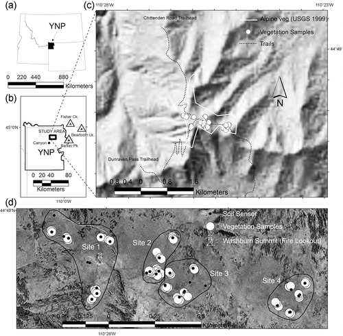
FIGURE 1 Overview of study area. Figures (a) and (b) locate Yellowstone National Park (YNP) and the study area. Figure (c) shows the topography of Mount Washburn. The extent of alpine vegetation is based on the vegetation classification of YNP by Despain (1990). Figure (d) shows the sampled sites (sites 1–4) on the four major Mount Washburn summits, vegetation plots, and soil sensors locations. A fire lookout is built on the main (highest) Washburn summit within site 1, which adjoins the summit weather station. Note the presence of supplementary soil sensors.

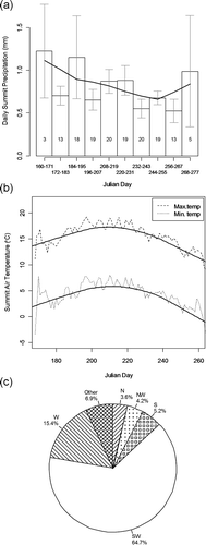
The plant-supporting surficial rock of the Washburn Range is from the Langford Formation, a unit of the Absaroka Volcanic Supergroup. The formation is composed primarily of hornblende and pyroxene andesite fragments, and was deposited 47–49 million years ago (Smedes and Protska, 1972). Glaciers, most recently from the Pinedale Glaciation, have scoured the Washburn Range and have contributed to the present-day rounded appearance of its ridges and northern slopes (Pierce, 1979). While year-round weather data is not available for the Washburn alpine, records from SNOTEL sites on adjacent mountain ranges suggest that its annual precipitation is near 800 mm (Aho, 2006) (Appendix, Fig. A1). Washburn summer climate (precipitation, temperature, and wind direction) has been measured at its summit lookout since 1965 (see Appendix, Fig. A2). These data indicate that summer precipitation on Washburn is lower than at adjacent alpine ranges. This may be due in part to Washburn's small mass and isolation which results in less extraction of moisture from rising air (Geiger et al., 2003). The average frost-free season length (number of days with minimum temps > 0 °C) on Washburn is 93 days. This is comparable to other nearby alpine and high subalpine sites (Aho, 2006). Summertime summit winds on Washburn are from southern aspects approximately 70% of the time (see Appendix, Fig. A2).

Methods

FIELD MEASUREMENTS

The major alpine environments of the Washburn alpine were sampled by selecting sites representative of six environmental nodes (cf. Poore, 1955; Lambert and Williams, 1962; Peterken, 1993). The nodes included three widespread ‘zonal’ environments (south slopes, ridges, and north slopes), and three more narrowly distributed ‘azonal’ environments (snowbanks, cliff ledges, and talus). We omitted east- and west-facing slopes, because of their scarcity along the lengthy Washburn ridgeline (which runs east to west), and because their environments are expected to be intermediate between north- and south-facing slopes (Geiger et al., 2003). We note that our choice of nodes was based on years of field work in the region and agrees with major alpine landscape components commonly identified in the Rockies (cf. Billings, 2000). Two plots representative of each node were randomly established on each of four summits (elev. 3032–3124 m) along Washburn's ridgeline (Fig. 1). Thus vegetation sampling was stratified with two plots representing each node at each summit. The exception was the cliff ledge node which was sampled only at the westernmost summit (Site 1).

The vegetation at each plot was sampled with ten 20 × 50 cm frames placed at 1 m intervals along its 10 m center line. The 10 m plot lines were located randomly within a node, perpendicular to the slope. The vegetation of each frame was characterized by listing the plant species present and visually estimating the cover of each (Daubenmire, 1959). Cover data from the 20 × 50 cm pseudoreplicates were combined (averaged) at each plot. Vegetation data was gathered in the first two weeks of July 2000 and 2001. Nomenclature follows Dorn (1992). Voucher specimens are housed at the Yellowstone National Park herbarium (YELLO, Gardiner, Montana).

Environmental data were also recorded at each plot. Elevations and locations were determined using Trimble^TM GeoExplorer 3 and Trimble^TM Pro XR receivers. Readings were differentially corrected against the Montana State University, and Idaho National Laboratory (INL) GPS base stations. Magnetic aspect (corrected for declination) and slope were measured using a Brunton compass. Potential annual direct incident radiation was calculated using slope, aspect, and latitude (McCune and Keon, 2002). Surface rock cover was measured as a percentage using 80 points located in the plot. This was done by recording rock hits for 8 points (nails) on a meter stick placed at 1 m intervals along the 10 m plot line. We assume that surface soil/rock ratio approximates that in the surface horizon. Soil samples were taken at all plot locations to measure soil C, N, P, pH, soil salinity (conductivity), and soil texture (i.e. % sand, % clay, % silt). Carbon was measured using both LECO (Nelson and Sommers, 1996) and Lawson ignition (Storer, 1984) methods. Soil nitrogen was determined using both LECO ignition (Nelson and Sommers, 1996) and Kjeldahl nitrogen (Bremner and Mulvaney, 1982) methods. Soil phosphorus was determined using the Bray method (Olsen and Sommers, 1982). Conductivity and pH were measured on 1∶1 water slurries with appropriate meters (Thomas, 1996). Soil texture was measured using the Boyoucous hydrometer method (Gee and Bauder, 1986).

To measure soil water and temperature in the nodal environments, one set of sensors were installed at each node on all four summits. The exception was the cliff ledge node where temperature and water sensors were installed in both cliff plots at site 1 (Fig. 1). Soil water and temperature sensors were installed at a depth of 15 cm. Sensors were read on 34 growing season days (late June to early October) over a five year period (2000–2004). Soil water sensors were Bouyoucos gypsum blocks (Beckman Instruments, P.O. Box 3100, 2500 Harbor Boulevard, Fullerton, California), and were read with a Delmhorst KS-D1 soil water (electrical resistance) meter. Resistance readings were converted to water potentials with appropriate calibration curves (Aho and Weaver, 2008). Temperatures sensors were thermocouples (Taylor and Jackson, 1986), and were read with an Omega HH-25TC thermocouple thermometer (http://www.Omega.com).

SOIL WATER AND TEMPERATURE MODELING

To describe the sigmoidal seasonal decline in soil water availability from saturated in the spring to dry at mid-summer (cf. Weaver, 1977), we used three parameter sigmoidal regressions to curve-fit, for each sensor, soil water potential as a function of date (cf. Larcher, 1977). The method of non-linear least squares was used for parameter estimation (Aster et al., 2005). We used the soil water models to estimate several ecologically relevant characteristics: i.e. number of days below particular water potentials (−0.12, −1.5 MPa), driest day, and wettest day.

To describe the unimodal seasonal rise and fall in soil temperature (cool in spring, warm in mid-summer, cool in fall), we used quadratic regressions to curve-fit, for each sensor, soil temperature against date. The models were used to derive important characteristics of seasonal soil temperature including the number of days when soil temperature was above 10 °C, maximum predicted temperature, and heatsum. Heatsum is the sum of daily temperatures (degree days) above 10 °C (Reader, 1983). Soil water potential and temperature curves for each sensor can be found in Aho (2006).

Community Analysis

To examine the structure of nodal communities, data from vegetation samples were ordinated with Non-Metric Multidimensional Scaling (NMDS; Kruskal, 1964). Although random starting points were also tried, the best (lowest stress) solutions resulted from using PCoA (Principal Coordinates Analysis) scores as initial starting points (Venables and Ripley, 2002). A tolerance of 1 × 10⁻⁷ was used with 200 iterations to create a scatterplot projection. To improve interpretability of NMDS axes, ordination configurations were rotated with PCoA so that the variance of points was maximized on the first dimension (Minchin, 1987). Bray-Curtis/Steinhaus dissimilarity (Bray and Curtis, 1957) was used to create the dissimilarity matrix.

Hierarchical agglomerative clustering was used to segment the vegetation continuum and demonstrate the distinctness of nodal communities. Linkage between plots was established using the flexible β method (Lance and Williams, 1967). We let β  =  −0.25 since this standard has previously provided effective cluster recovery in regional alpine vegetation data sets (Aho et al., 2008). Wishart's objective function (Wishart, 1969) was used to scale the cluster dendrogram. Bray-Curtis/Steinhaus dissimilarity (Bray and Curtis, 1957) was used to create the dissimilarity matrix. The optimal classification solution was found by pruning the dendrogram to create the 19 simplest classification solutions (2–20 clusters), then evaluating these results with 7 classification evaluators. For detail on these procedures see Aho et al. (2008).

The relationship between nodal communities and environment variables was examined with summary statistics, multivariate inferential analyses, and by plotting presumptive factors onto the ordination diagram. Multivariate regressions quantified the capacity of environmental variables to explain variability in the summarized community space of the ordination after accounting for spatial proximity. In particular, the partial r ² of an environmental predictor was determined by adding it to a model already containing spatial variables (UTMs) and calculating the decrease in the multivariate residual sum of squares; i.e. SSEs (Kutner et al., 2005; McArdle and Anderson, 2001). Multivariate pseudo-SSEs for the reference and nested models were derived using the method of NP-MANOVA (Anderson, 2001; McArdle and Anderson, 2001). P-values for regression predictors were derived using permutation procedures based on the NP-MANOVA pseudo-F statistic (Oksanen et al., 2008). The explanatory power of environmental variables and their community impacts were graphically depicted with vector arrows overlaid on the ordination (i.e. vector fitting; Oksanen et al., 2008).

SOFTWARE

Classifications were created using PC-ORD (McCune and Mefford, 1999). Algorithms for classification evaluators, ordinations, and multivariate inferential procedures were coded in R (R Development Core Team, 2008), often using existing functions in the MASS (Venables and Ripley, 2002) and vegan (Oksanen et al., 2008) libraries.

Results

NODAL COMMUNITIES

A consensus of classification evaluators indicated that six clusters was the optimal number of classes for the agglomerative classification of community data (cf. Aho et al., 2008). The six clusters corresponded to the six sampled nodes, demonstrating the distinctiveness of the nodal communities. A two dimension NMDS ordination was sufficient to summarize variability in species space [Stress  =  12.9, Linear r ²  =  0.94, Non-linear r ²  =  1 − (Stress/100)²  =  0.983]. When treated as a categorical variable, the six clusters explained 86% of the ordination variability after accounting for spatial proximity (Table 1, Fig. 2).

FIGURE 2 NMDS ordination and results of NP-MANOVA analyses. (a) Communities indicated with spider diagrams. Ellipses indicate 95% confidence intervals around cluster centroids. Community 1  =  Elymus scribneri talus (ELSC), community 2  =  Senecio canus–Astragalus kentrophyta (SECA-ASKE), community 3  =  Erigeron rydbergii–Oxytropis lagopus (ERRY-OXLA), community 4  =  Carex elynoides–Astragalus alpina (CAEL-ASAL), community 5  =  Carex paysonis–Artemisia scopulorum (CAPA-ARSC), community 6  =  Arnica rydbergii (ARRY). (b) Environmental vectors are scaled by their partial r ²'s (Table 1). The direction of the arrows indicates the direction of most rapid increase for variables in the ordination. Environmental variables are: P  =  phosphorus (mg kg⁻¹), C  =  % soil carbon, N  =  % soil nitrogen, Elevation  =  elevation (m), Slope  =  slope(degrees), Aspect  =  degrees from north, Soil  =  % cover of surface soil, EC  =  soil conductivity (mmhos cm⁻¹), sand  =  % sand content of soil, silt  =  % silt content of soil, Temperature  =  soil temperature (number of summer days > 10 °C), H₂O  =  length of water stress–free season (number of summer days > −0.12 Mpa). Note that while they have different overlays, the ordinations shown in (a) and (b) are identical. Final stress for 2D NMDS solution  =  12.9.

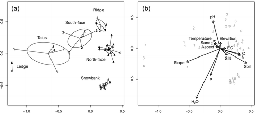
TABLE 1 Association of the NMDS ordination solution and environmental variables (see Fig. 2b).

We assigned diagnostic species to the six nodal classes and summarized their communities with respect to species cover and constancy (Table 2). More elaborate descriptions of the nodal communities and an extensive literature search evaluating their relationship to similar alpine ecosystems can be found in Aho (2006). A brief plant community summary also appears in the Appendix to this paper.

TABLE 2 Summary relevé table for the six nodal community types^a. The two-character cipher^b included in each cell indicates constancy (% of sites within the community that contain the species), and cover. Bolded cells indicate constancy ≥ 30%.

The ordination (Fig. 2) shows relationships of the nodal communities to each other. Moving from the lower left to the upper right hand side of the diagram reveals a series of communities representing ledge, talus, south-face, and ridgetop nodes (Fig. 2). While it is most similar to north-slope communities, the separation of the snowbank node from this overall gradient indicates its uniqueness (cf. Billings and Bliss, 1959).

The nodal communities were distinct with respect to cover and diversity (Table 3). Mean vegetation cover was highest on the dry dense turf of the north-facing node (97%) and on snowdrift sites (88%), lower on rocky south-face and ridge nodes (41%–65%), and lowest on ledges (15%) and talus (9%) (Table 3). Species richness (mean/total) was highest in north-facing turf (22/51) and snowbanks (26/55), lower on south-face and ridge nodes (16/27 and 17/32) and talus (9/21), and lowest on ledges (4/5). Diversity parallels cover and species richness with lowest diversity on ledges, (0.45/0.76 for Simpson and Shannon-Wiener indices, respectively), and highest diversity on north-faces (0.90/2.56) (Table 3). The heterogeneity of talus vegetation is demonstrated by its high β-diversity (average Bray-Curtis dissimilarity; McCune and Grace, 2002) of 1.44 compared to 0.43–1.34 in other communities (Table 3).

TABLE 3 Comparison of environments of the six nodal communities^a on Mount Washburn. Standard errors are included with sample means.

NODAL ENVIRONMENTS

Multivariate regressions and permutation analyses revealed that environmental variables were strongly associated with nodal community patterns (Fig. 2b, Table 1). Variables most strongly correlated with plant community structure in the ordination after accounting for spatial location were soil water seasonality (partial r ²  =  0.44, permutation p-value from NP-MANOVA < 0.001), slope (partial r ²  =  0.29, p < 0.001), soil cover (partial r ²  =  0.24, p < 0.001), soil N (partial r ²  =  0.17, p  =  0.001), C ( partial r ²  =  0.17, p  =  0.001), and pH (partial r ²  =  0.23, p < 0.001) (Table 1).

Environmental variation on the first (horizontal) ordination axis was strongly associated with slope, aspect, and related qualities (Fig. 2). Slope decreased from ledges (32°) and talus (30°) though south slopes (22°), north-facing snowbanks (18°), north slopes (19°), and plateau-like ridgetops (13°; Fig 2, Table 3). Aspect (degrees from north) paralleled slope and fell from south-facing ledges, talus, and south slopes (170°, 137°, 127°) to ridgetops, north slopes, and snowbanks (87°, 64°, 40°; Table 3). Annual incident solar radiation (MJ cm⁻² yr⁻¹) fell similarly from ledge, talus, and south slopes (1.0, 0.94, 0.93) to ridgetops, north slopes, and snowbanks (0.84, 0.79, 0.73; Table 3).

Environmental variation on the second (vertical) axis was strongly associated with soil temperature, water relations, and nutrient status (Fig. 2). Whether one considers heat sum, observed maximum temperature, or the number of warm days (temperature >10 °C), soil temperatures drop from south slopes and ridges to north-facing turf and snowbanks (Table 3). Indicators of water availability (water delivery, water storage capacity, and onset of summer water stress) generally increase from south slopes and ridges to turf and snowbanks. Water delivery can be measured indirectly as accumulation of silt which is blown with drifting snow. Silt (%) increases from talus (30) to ledges (32) to south slopes (32) to ridges (33) to snowbanks (39) and north-facing slopes (40) (Table 3). Water storage capacity, indexed by soil cover (%) in the surface horizon, increased in parallel (Table 3). Water delivered in excess of soil storage capacity results in leaching of exchangeable bases and can be indexed by soil acidity. Soil pH falls from south slopes and ridges (6.7–7.0) to north-facing turf and snowbank (6.5, 5.7). While the length of the water stress season (soil H₂O, Fig. 2) parallels the second axis and separates snowbanks (which have a particularly late onset of water stress) from south slopes, ridges, and north-facing turf, it does not distinguish the latter three nodes (Table 3). Nutrients (N and P) and soil organic matter increase from south-facing nodes (talus, ledge, and south slope) to ridges, north-facing turf, and snowbanks (Table 3). Material blown northward with snow can be indexed with silt accumulation (see above). For example, phosphorus, which is tightly bound to clay and silt, rises from ridges and south slopes and ridges (21, 23 mg kg⁻¹) to north-facing turf and snowbanks (29, 36 mg kg⁻¹). Soil nitrogen strongly increases from south-facing to north-facing nodes. Soil N (%Kjeldahl, %LECO) increases from ledges (0.07, 0.08) to talus (0.11, 0.12) to south faces (0.16, 0.16) to ridgetops (0.31, 0.41) to snowbanks (0.43, 0.51) and dense turf (0.62, 0.72) (Table 3).

Discussion

In this paper we describe nodal alpine communities, environments, and their relationships on Mount Washburn. We acknowledge that multivariate and univariate differences among nodes are largely due to a conscious effort to sample within pre-defined strata representing disparate ecosystems. Our investigation was not designed to find average conditions on Washburn but to find (1) if ecosystem nodes (poles) differ, (2) how they differ, and (3) why they differ. In the discussion below we pursue these topics by describing the major environmental gradients among the nodes, explaining how vegetation responds to these gradients, and from these conclusions constructing a model for ecosystem evolution.

ENVIRONMENTAL GRADIENTS

The nodal ecosystems were related to each other on the axes of an ordination (Fig. 2). Because the two axes adequately described variation in the communities (non-metric r ²  =  0.98), we deduce that community variation is largely due to two environmental factors or factor complexes. We previously demonstrated that the first dimension (which is strongly correlated with variability in slope and aspect) distinguishes steep south-facing nodes: (talus, south faces, ledge) from more gradually sloped north-facing nodes (north faces and snowbanks). Steep southern slopes, resulting from the formation of the Yellowstone Caldera (Parsons, 1978), have less stability and greater wind exposure than north-facing sites. Both of these factors inhibit plant growth and prevent soil development. Gradients on the second (vertical) dimension (Fig. 2) are more complex but are equally important in explaining the distribution of communities. This dimension differentiates resource-poor nodes (those with low soil water and nutrient storage) from resource-rich nodes; i.e. it distinguishes south-facing and ridge nodes from north-facing nodes. In addition, the second dimension separates early-drying north-facing turf sites from late-drying north-facing snowbank sites (Fig. 2). Because it falls from south-facing nodes to north-facing nodes, soil temperature is negatively associated with measured resources (e.g. water, nutrients, soil cover). We consider soil water, nutrients, and temperature and their effect on nodal communities below.

Water

Water is more available on north- than south-facing slopes. This is true for three reasons. First, snow deposited on south-facing slopes is moved to north-facing lee slopes by continual winds from the south. This hypothesis is supported by the large amounts of loess on north-facing slopes, particularly at north-facing snowbank sites (Table 3). Second, evaporation and sublimation of snow is relatively high on south-facing slopes due to both wind exposure (Neuwinger, 1980; Oberbauer and Billings, 1981), and increased radiation (Table 3; Geiger et al., 2003). Third, as a result of more abundant soils, north slopes have greater water storage capacity than south slopes, and thus their ‘moist season’ is extended further into summer.

Our measurement of seasonal soil water adds a biotic dimension to the water story. Despite greater supply and storage, north-facing nodes become water depleted (surface soil water potential drops below −1.5 MPa) at the same time as ridgetop and south-facing nodes (Table 3). We attribute early depletion to high vegetation cover (97%) on north slopes, resulting in high levels of transpiration relative to warmer but lower cover ridge (65%) and south-facing (41%) sites (Table 3). In addition, surface soils of productive north-facing turf are water depleted long (18 days) before less productive snowbank sites (Table 3). Depletion is postponed on drift sites relative to high-transpiration north-facing turf because, until it is gone, snow cover at snowbank sites simultaneously prevents transpiration and keeps soils at field capacity. The delay in water depletion and low sun exposure at snowbank sites also work together to offset the growing season later into the summer. As a result of postponement of growth to the warmest part of summer, the water use efficiency and resultant production of snowbank communities are probably lower than at north-facing turf (cf. Weaver and Collins, 1977; Lambers et al., 1998). Talus and ledge nodes also dry much later than north-facing turf, south slopes, and ridges (Table 3). We attribute this to the fact that these nodes have both low vegetation cover (resulting in low levels of transpiration) and receive vadose water from uphill sites (cf. Körner, 2003, p. 132, and Theodose and Bowman, 1997). While our data are also from surface soils (15 cm), we expect similar but lagging dynamics in subsurface soils (cf. Daubenmire, 1968; Weaver, 1977).

Nutrients and Soils

Nutrient supplies (e.g. soil N and P) were probably equal among nodes immediately following the last glaciation. Presently, however, nutrient storage is greater at north-facing nodes (Table 3). North-facing slopes support nutrient accumulation for three reasons: (1) nutrient-bearing loess is blown to north-facing lee slopes with snow and soil, (2) gradual north slopes are less susceptible to nutrient loss by erosion, and (3) resultant increases in plant productivity support a positive feedback loop that increases slope stabilization, and nutrient inputs and retention over time.

The distribution of the essential nutrients P and N (e.g. Seastedt and Vaccaro, 2001) illustrates the dynamics of nodal nutrient supply. Phosphorus generally increases from south and ridge sites to north-facing nodes (Table 3). This is surely due to eolian transport from wind-scoured south faces to north-facing lee slopes, coupled with binding of P by fine textured north-facing soils (Table 3). Nitrogen increases dramatically from south- to north-facing slopes, but decreases slightly at snowbank sites (Table 3). N accumulation can be attributed to N₂ fixation from free-living cyanobacteria, whose presence increases with alpine water availability (Wojciechowski and Heimbrook, 1984), nodulated legumes, e.g. Lupinus argenteus, on north-facing turf (cf. Goergen et al., 2009), and deposition of organic matter (cf. Bowman, 1992). N/P ratios fall slightly from north-facing turf to snowbanks because N is more easily leached than P by large amounts of snowbank meltwater (cf. Chapin, 1980).

Soil C increases from south faces to ridge to turf and declines under snowbanks (Table 3). While it is not a nutrient, organic matter (OM) has four important roles. First, it increases the water storage capacity of the soil (Isard, 1986). Second, it adsorbs nutrient cations (e.g. K⁺, Ca²⁺; Lambers et al., 1998, p. 241), increasing their storage. Third, essential nutrients (e.g. N, P, S) are covalently bound to OM, and it retains them in an unleachable form preceding decomposition. Fourth, while soil nutrient accumulation from OM does not equate with nutrient availability, OM contains compounds, including chelating agents and organic acids, which make nutrients more available to plants (Delgado and Follett, 2002).

Temperature

Soil temperature falls from south-facing ledge sites through south slopes, ridges, to north-facing turf and snowbank sites. Steep south-facing ledge sites are especially warm because their soils are more directly exposed to radiation (Table 3). In contrast, despite their relatively steep slopes, southern aspects, and resultant high radiation inputs, soil temperatures under talus were comparable to those of north-facing nodes (Table 3). This is surely due to the heavy rock mulch that shields their soils from incident radiation (cf. Körner, 2003, p. 63).

FLORISTICS

In general the Washburn alpine is similar to alpine flora of other regions (i.e. Cooper et al., 1997; see Aho, 2006, for extensive comparisons). However, there are several exceptions. Of particular note, Bupleurum americanum, Eritrichium nanum, and Dryas octopetala, and one major genus, Trifolium (e.g. T. dasyphyllum, T. haydenii, and T. parryi) are absent on Washburn although they are often dominant in adjacent alpine areas including the granitic Beartooth Plateau (Lackschewitz, 1994; Aho, 2006). Hypothetically these absences may be due to a number of factors including Washburn's andesitic substrate, and its insular characteristics (small size and isolation). Two of the listed missing species are documented calciophiles, D. octopetala (Bamberg and Major, 1968; Komárková, 1979; Willard, 1979), and E. nanum (Bamberg and Major, 1968). D. octopetala, B. americanum, and E. nanum are also missing from andesitic alpine areas in the Southern Rockies (Rottman and Hartman, 1985; Baker, 1983) and coastal cordilleras (Hunter and Johnson, 1983). D. octopetala occurs, albeit rarely, in the nearby andesitic Northern Absarokas and Gallatin ranges (Aho, 2006). The genus Trifolium is also missing from the Northern Absarokas (Aho, 2006). However its presence/absence appears unrelated to andesitic substrates since it is also missing from the granitic Tetons (Spence and Shaw, 1981) while occurring on the andesitic soils in the Southern Absarokas (Thilenius and Smith, 1985).

Community Composition

The Washburn flora varied among nodes with respect to both guilds and individual species. With respect to guilds, rocky ridge sites were dominated by tap rooted cushion plants, while north-facing soil-rich sites were dominated by diffuse rooted graminoids. Sun-warmed but nutrient deficient ledges supported upright relatively fragile plant life forms, e.g. Arnica rydbergii. Dominant species also varied along nodal gradients (Table 2). Among numerous examples, Carex paysonis, Aster foliaceus, and Artemisia scopulorum were dominant at snowbanks, but occurred infrequently at other nodes.

Species richness and cover increased with decreasing rockiness and increasing water availability and nutrient storage (Table 3). In contrast, both were negatively associated with indices of soil temperature, i.e. warm southern nodes had the lowest richness and cover. While a positive association of vegetation richness and cover to temperature has been demonstrated for most terrestrial systems (e.g. Holdridge, 1947; Leith, 1975), this effect is overridden, within the Washburn alpine, by the importance of soil and water availability, and nutrient storage.

WASHBURN ECOSYSTEM EVOLUTION

Our observations have led us to conclude that geological and biological processes have combined to increase environmental resources for some nodes at the expense of others. At the end of the last glaciation (∼10,000 yr. BP), it is likely that soil development among nodes was relatively homogeneous with respect to depth, water-holding capacity, and nutrient accumulation (Pierce, 1979). Over the millennia, however, winds have continually transported snow and soil components from southern to northern lee slopes (cf. Billings, 1973; Pelletier and Cook, 2005; see also Appendix). As a result of eolian water and soil deposition, and steep southern slope erosion, water and nutrient storage and availability has continually increased on north-facing slopes compared to southern slopes (cf. Lerman and Maybeck, 1988, p. 133). Because of increased resources vegetation growth has increased. This increased productivity has in turn magnified the capture and stabilization of soils and deposition of organic matter, which has further increased luxuriance of north face lee vegetation in a biologically driven positive feedback loop (cf. Holtmeier, 2003).

Our evolutionary model reflects the characteristics of a number of proposed models for alpine ecosystems. For instance eolian transport processes for water, organic matter, and minerals, are important to both our model and the recently proposed alpine landscape continuum model (LCM) of Seastedt et al. (2004). Similarly, inter-nodal transport of water (from southern to northern nodes on Washburn) is implicit in the mesotopographic model of Billings (1973), which predicts that alpine communities are the product of snow cover gradients produced by interactions of wind exposure and topography. On Washburn, biologically driven ecosystem controls occur from both short term and long term perspectives. In the short term seasonal soil water availability on Washburn is biologically controlled as a result of transpiration. This is evident in the short periods of water surplus which occur at the densely vegetated north-facing node despite its water subsidies. In the long term north-facing nodes are a sink for eolian inputs of water, soil, and minerals, which are captured and assimilated by vegetation in a positive feedback loop. Wind-blown nodes (south faces and ridges) and snowdrift sites both had poorly developed soils compared to the north-facing node. This is in strong agreement with predictions of the model of Burns and Tonkin (1982) which attributed such patterns to differences in rates of biological driven soil formation. Similar biological ecosystem controls are acknowledged in the state factor model of Jenny (1941) and Admundson and Jenny (1997).

Conclusions

Alpine topographic facets (nodes) differ in environment and, as a result, in vegetation composition and vegetation qualities. Conversely, vegetation influences its environment through mechanisms including feed-back loops which affect both biotic and abiotic ecosystem processes. We found that resources (e.g. water availability and nutrient storage) increased from south- to north-facing nodes, while temperatures fell. In addition, the seasonality of resource availability differed among nodes. For instance, despite greater water inputs and storage, soils of north-facing turf dried concurrently with south-facing and ridge sites. The early drying of north-facing turf is likely due to its high vegetation cover and resultant high transpiration. Snowbank, talus, and cliff sites dried last due to both lower transpiration and later delivery of snowmelt and vadose water. Nutrient accumulation generally parallels increased water availability, is confounded with it, and likely reinforces the influence of water.

The vegetation of the nodes was distinct (Fig. 2, Table 2) although communities surely intergraded on gradients connecting the nodes. Table 2 demonstrates shifts in the distributions of taxa and guilds on environmental gradients, e.g. the transition from low cover forb vegetation, on sun-warmed wind-blown sites, to high-cover graminoid dominance on cooler wind-sheltered north-facing sites. We propose that increases in soil deposition along the water/nutrient gradient support a positive feedback loop in which the soil and water trapping and storage capacity of north-facing lee slopes have increased over time as increasing vegetation has captured and generated more organic matter (Jenny, 1941; Admundson and Jenny, 1997; Holtmeier, 2003).

Acknowledgments

Thanks to D. Despain (U.S. Geological Survey, retired), R. Williams (Idaho State University), M. Hektner (Yellowstone National Park–National Park Service), J. Whipple (YELLO), T. Seipel (field assistance), C. Seibert (Montana State University), the YNP fire cache, and three anonymous AAAR reviewers. This research was made possible in part with a grant from the National Park Service (YNP-NPS YELL-05116) and by assistantships from Montana State University.

Appendix

A Brief Summary Of Washburn Nodal Communities

The three zonal nodes (south face, ridge, and north face) contained distinctive communities. The Senecio canus–Astragalus kentrophyta (SECA-ASKE) type is an open forb-rich community usually occurring on warm, rocky, south-facing sites with associates Arenaria obtusiloba, Cerastium arvense, Erigeron compositus, Lomatium cous, Phlox pulvinata, and Sedum lanceolatum. The Erigeron rydbergii–Oxytropis lagopus (ERRY-OXLA) type is an open cushion/taprooted plant community of rocky ridgetops which often includes Arenaria obtusiloba, Cerastium arvense, Erigeron compositus, Lomatium cous, Phlox pulvinata, and Sedum lanceolatum. Conversely, the Carex elynoides–Astragalus alpina (CAEL-ASAL) community is a dense, dry turf which occupies north-facing sites with moderate snow accumulation and contains a large number of species including Luzula spicata, Poa rupicola, Arenaria obtusiloba, Cerastium arvense, Potentilla diversifolia, and Sedum lanceolatum.

There were also three azonal communities representing the three sampled azonal nodes (snowbank, talus, and ledge). The snowbank node was occupied by the Carex paysonis–Artemisia scopulorum (CAPA-ARSC) type, a graminoid-dominated community of localized snowbank sites. Associates include Carex phaeocephala, Festuca brachyphylla, Luzula spicata, Achillea millefolium, Arenaria obtusiloba, Cerastium arvense, Erigeron simplex, Polygonum bistortoides, and Stellaria monantha. On steep sites one finds two little-studied azonal communities. The Arnica rydbergii (ARRY) type is a low diversity forb community of south-facing cliff ledge seeps. The Elymus scribneri (ELSC) type is a highly heterogeneous community of talus sites with infrequent associates including Erigeron compositus and Cerastium arvense.

FIGURE A1 Climate diagrams (cf. Walter and Leith, 1967) for (a) Canyon Village and (b) Parker Peak SNOTEL stations (see Fig. 1 for locations). Raw climate data provided by the Western Regional Climate Center (WRCC, 2008). The upper line shows average monthly precipitation; the lower humped line shows average mean monthly temperature. The vertically hatched area between them indicates the months that precipitation exceeds evaporation. Text at the figure top gives the following: length of records in years for temperature and precipitation, respectively [in brackets], latitude/longitude, station name, elevation, average yearly precipitation, and overall mean temperature. Average daily maximum temperature of the warmest month and average daily minimum temperature of the coldest month are indicated on the temperature axis. The white area in the strip across the bottom of the figure indicates the frost-free period.

FIGURE A2 Growing season weather data from the Washburn summit. (a) Mean summer precipitation (1965–1969, 1990–2008). Numbers within the bars are the number of years of data used to compute the means. Error bars are standard errors. (b) Mean minimum and maximum temperature (1965–1969, 1990–2008). (c) Wind direction for 1965–1969, 1990–1997, and 2001–2008 (N  =  north, S  =  south, W  =  west). Localized weighted scatterplot smoother (lowess) lines are superimposed in (a) and (b). Raw data provided by the National Park Service.

References Cited

- Admundson, R. and H. Jenny . 1997. On a state factor model of ecosystems. BioScience 47:536–543.
- Aho, K. 2006. Alpine Ecology and Subalpine Cliff Ecology in the Northern Rocky Mountains PhD dissertation. Montana State University, Bozeman, Montana.
- Aho, K. and T. Weaver . 2008. Measuring soil water potential with gypsum blocks: calibration and sensitivity. Intermountain Journal of Sciences 14 1–3:51–60.
- Aho, K. , D. Roberts , and T. Weaver . 2008. Using geometric and non-geometric internal evaluators to compare eight vegetation classification methods. Journal of Vegetation Science 19:549–562.
- Anderson, M. J. 2001. A new method for non-parametric multivariate analysis of variance. Australian Ecology 26:32–46.
- Aster, R. C. , B. Borchers , and C. H. Thurber . 2005. Parameter Estimation and Inverse Problems. Burlington, Massachusetts Elsevier Academic Press.
- Baker, W. L. 1983. Alpine vegetation of Wheeler Peak, New Mexico U.S.A.: gradient analysis, classification and biogeography. Arctic and Alpine Research 15 2:223–240.
- Bamberg, S. A. and J. Major . 1968. Ecology of the vegetation and soils associated with calcareous parent materials in three alpine areas in Montana. Ecological Monographs 38:127–167.
- Billings, W. D. 1973. Arctic and alpine vegetations: similarities, differences, and susceptibility to disturbance. BioScience 23:697–704.
- Billings, W. D. 2000. Alpine vegetation. In: Barbour, M. D. and W. D. Billings . North American Terrestrial Vegetation. Second edition. Cambridge Cambridge University Press. 536–572.
- Billings, W. D. and L. C. Bliss . 1959. A snowbank alpine environment and its effects on vegetation, plant development, and productivity. Ecology 40 3:388–397.
- Bowman, W. D. 1992. Inputs and storage of nitrogen in winter snowpack in an alpine ecosystem. Arctic, Antarctic, and Alpine Research 24 3:211–215.
- Bray, R. J. and J. T. Curtis . 1957. An ordination of upland forest communities of southern Wisconsin. Ecological Monographs 27:325–349.
- Bremner, J. M. and C. S. Mulvaney . 1982. Nitrogen—Total. In Page, A. L. Methods of Soil Analysis. Part 2: Chemical and Microbiological Properties. Second edition. Madison, Wisconsin American Society of Agronomy and Soil Science Society of America. 595–622.
- Bryant, D. M. , E. A. Holland , T. R. Seastedt , and M. D. Walker . 1998. Analysis of litter decomposition in an alpine tundra. Canadian Journal of Botany 76:1295–1304.
- Burns, S. F. and P. J. Tonkin . 1982. Soil geomorphic models and the spatial distribution and development of alpine soils. In Thorn, C. E. Space and Time in Geomorphology. London George Allen and Unwin. 25–44.
- Chapin III, F. S. 1980. The mineral nutrition of wild plants. Annual Review of Ecology and Systematics 11:233–260.
- Cooper, S. V. , P. Lessica , and D. Page-Dumroese . 1997. Plant Community Classification for Alpine Vegetation on the Beaverhead National Forest, Montana. Ogden, Utah Intermountain Research Station, U.S. Forest Service, U.S. Department of Agriculture, General Technical Report INT-GTR 362.
- Daubenmire, R. 1959. A canopy coverage method of vegetation analysis. Northwest Science 33:43–64.
- Daubenmire, R. 1968. Soil moisture in relation to the vegetation distribution in the mountains of northern Idaho. Ecology 49:431–437.
- Delgado, J. A. and R. F. Follett . 2002. Carbon and nutrient cycles. Journal of Soil and Water Conservation 57 6:455–464.
- Despain, D. G. 1990. Yellowstone Vegetation. Consequences of Environment and History in a Natural Setting. Boulder, Colorado Rinehart Inc. Publishers.
- Dorn, R. D. 1992. Vascular Plants of Wyoming. Cheyenne, Wyoming Mountain West Publishing.
- Feeley, T. , M. A. Cosca , and C. R. Lindsay . 2002. Petrogenesis and implications of calc-alkaline cryptic-hybrid magmas from Washburn Volcano, Absaroka Volcanic Province, USA. Journal of Petrology 43 3:663–703.
- Gee, G. and J. Bauder . 1986. Particle size analysis. In: Klute, A. Methods of Soil Analysis I: Physical and Mineralogical Methods. Madison, Wisconsin American Society of Agronomy and Soil Science Society of America. 383–411.
- Geiger, R. , R. H. Aeon , and P. Todhunter . 2003. The Climate near the Ground. Sixth edition. Lanham, Maryland Rowman and Littlefield.
- Goergen, E. , J. C. Chambers , and R. Blank . 2009. Effects of water and nitrogen availability on nitrogen contribution by the legume, Lupinus argenteus Pursh. Applied Soil Ecology 42 3:200–208.
- Gotelli, N. J. and A. M. Ellison . 2004. A Primer of Ecological Statistics. Sunderland, Massachusetts Sinauer.
- Holdridge, L. R. 1947. Determination of world plant formations from simple climatic data. Science 105:367–368.
- Holtmeier, F. K. 2003. Mountain Timberlines: Ecology, Patchiness, and Dynamics. Dordrecht, Netherlands Kluwer Academic Publishers.
- Hunter, K. B. and R. E. Johnson . 1983. Alpine flora of the Sweetwater Mountains, Mono County, California. Madrono 30:89–105.
- Isard, S. A. 1986. Factors influencing soil moisture and plant community distribution on Niwot Ridge, Front Range, Colorado, USA. Arctic and Alpine Research 18 1:83–96.
- Jaeger, C. H. , R. K. Monson , M. C. Fisk , and S. K. Schmidt . 1999. Seasonal partitioning of nitrogen by plants and soil microorganisms in an alpine ecosystem. Ecology 80 6:1883–1891.
- Jenny, H. 1941. Factors of Soil Formation. New York McGraw-Hill.
- Kokaly, R. F. , D. G. Despain , R. N. Clark , and K. E. Livo . 2003. Mapping vegetation in Yellowstone National Park using spectral feature analysis of AVIRIS data. Remote Sensing of the Environment 84 3:437–456.
- Komárková, V. 1979. Alpine Vegetation of the Indian Peaks Area, Front Range, Colorado Rocky Mountains PhD dissertation. University of Colorado, Boulder, Colorado.
- Körner, C. 2003. Alpine Plant Life: Functional Plant Ecology of High Mountain Ecosystems. Second edition. Berlin Springer-Verlag.
- Kruskal, J. B. 1964. Nonmetric multidimensional scaling: a numerical method. Psychometrika 29:115–129.
- Kutner, M. H. , C. J. Nachtsheim , J. Neter , and W. Li . 2005. Applied Linear Statistical Models. Fifth edition. Boston McGraw-Hill.
- Lackschewitz, K. H. 1994. Beartooth alpine flora. In Anderson, B. Beartooth Country: Montana's Absaroka and Beartooth Mountains. Helena, Montana Unicorn Publishing. 105–113.
- Lambers, H. , F. S. Chapin III , and T. L. Pons . 1998. Plant Physiological Ecology. New York Springer-Verlag.
- Lambert, L. M. and W. T. Williams . 1962. Multivariate methods in plant ecology: IV. Nodal analysis. Journal of Ecology 50 3:775–802.
- Lance, G. N. and W. T. Williams . 1967. A general theory of classification sorting strategies II. Clustering systems. Computer Journal 10:271–277.
- Larcher, W. 1977. Ergebnisse des IBP-Projekts “Zwergstrauchheide Patscherkofel”. Sitzungsberichte der Öesterr. Akademie der Wissenschaften, Mathematisch-Naturwissenschaftliche Klasse I 186:309–328.
- Leith, H. 1975. Modeling primary productivity of the world. In Lieth, H. and R. H. Whittaker . Primary Productivity of the Biosphere. New York Springer-Verlag. 236–263.
- Lerman, A. and M. Maybeck . 1988. Physical and Chemical Weathering in Geochemical Cycles. New York Springer-Verlag.
- Losleben, M. 2009. Saddle (3525 m) Climate Station: CR23X Data. (http://culter.colorado.edu/exec/.extracttoolA?sdlcr23x.ml).
- MacArthur, R. H. and J. W. MacArthur . 1961. On bird species diversity. Ecology 42:594–598.
- Marr, J. W. , A. W. Johnson , W. S. Osburn , and O. A. Kron . 1968. Data on Mountain Environments II: Front Range, Colorado, Four Climate Regions University of Colorado Studies, Series in Biology. 28.
- Mattson, D. J. and R. H. Reinhart . 1990. Whitebark Pine on the Mount Washburn Massif, Yellowstone National Park U.S. Forest Service General Technical Report INT: ISSN: 07481209, 106–117.
- McArdle, B. H. and M. J. Anderson . 2001. Fitting multivariate models to community data: a comment on distance-based redundancy analysis. Ecology 82:290–297.
- McCune, B. and J. B. Grace . 2002. Analysis of Ecological Communities. Gleneden Beach, Oregon MjM Software Design.
- McCune, B. and D. Keon . 2002. Equations for potential annual direct radiation and heat load. Journal of Vegetation Science 13:603–606.
- McCune, B. and M. S. Mefford . 1999. PC-ORD: Multivariate Analysis of Ecological Data. Version 4. Gleneden Beach, Oregon MjM Software Design.
- Minchin, P. R. 1987. An evaluation of relative robustness of techniques for ecological ordinations. Vegetatio 71:145–156.
- Nelson, D. W. and L. E. Sommers . 1996. Total carbon, organic carbon, and organic matter. In Sparks, D. L. Methods of Soil Analysis. Part 3. Chemical Methods. Madison, Wisconsin American Society of Agronomy and Soil Science Society of America. 961–1010.
- Neuwinger, I. 1980. Erwärmung, Wasserrückhalt and Erosionsbereitschaft subalpiner Böden. Mitt. Forstl. Bundes.-Veruchsanst. (Wein) 129:113–144 (cited in Körner, 2003).
- Oberbauer, S. F. and W. D. Billings . 1981. Drought tolerance and water use by plants along an alpine topographic gradient. Oecologia 50:325–331.
- Oksanen, J. , et al 2008. Vegan: Community Ecology Package. R package version 1.15-0 (http://cran.r-project.org/, http://vegan.r-forge.r-project.org).
- Olsen, S. R. and L. E. Sommers . 1982. Phosphorus. In Page, A. L. , et al Methods of Soil Analysis Part 2. Agronomy Monograph 9. Second edition. Madison, Wisconsin American Society of Agronomy and Soil Science Society of America. 403–430.
- Parsons, W. H. 1978. K/H Geology Field Guide Series: Middle Rockies and Yellowstone. Dubuque, Iowa Kendall/Hunt Publishing.
- Pelletier, J. D. and J. P. Cook . 2005. Deposition of playa windblown dust over geologic time scales. Geology 33 11:909–912.
- Peterken, G. F. 1993. Woodland Conservation and Management. New York Springer-Verlag.
- Pierce, K. 1979. History and Dynamics of Glaciation in the Northern Yellowstone National Park Area U.S. Geological Survey Professional Paper 729F.
- Podruzny, S. R. 1999. Grizzly Bear Use of Whitebark Pine Habitats in the Washburn Range Masters thesis. Montana State University, Bozeman, Montana.
- Poore, M. E. D. 1955. The use of phytosociological methods in ecological investigations. I. The Braun-Blanquet system. II. Practical issues involved in an attempt to apply the Braun-Blanquet system. III. Practical application. Journal of Ecology 43:226–244, 245–269, 606–651.
- R Development Core Team 2008. R: a Language and Environment for Statistical Computing. Vienna, Austria R Foundation for Statistical Computing. ISBN 3-900051-07-0 (http://www.r-project.org).
- Reader, R. J. 1983. Using heatsum models to account for geographic variation in floral phenology of two ericaceous herbs. Journal of Biogeography 10:47–54.
- Richmond, G. , W. Mullenders , and M. Coremans . 1978. Climatic Implications of Two Pollen Analyses from Newly Recognized Rocks of Latest Pliocene Age in the Washburn Range, Yellowstone National Park, Wyoming U.S. Geological Survey Bulletin 1455.
- Rottman, M. L. and E. L. Hartman . 1985. Tundra vegetation of three cirque basins in the northern San Juan Mountains, Colorado. Great Basin Naturalist 45:87–93.
- Seastedt, T. R. and L. Vaccaro . 2001. Plant species richness, productivity, and nitrogen and phosphorus limitations across a snowpack gradient in alpine tundra, Colorado, USA. Arctic, Antarctic and Alpine Research 33 1:100–106.
- Seastedt, T. R. , W. D. Bowman , N. Caine , D. McKnight , A. Townsend , and M. W. Williams . 2004. The landscape continuum: a model for high elevation ecosystems. Bioscience 54 2:111–121.
- Shultz, C. 1969. Mount Washburn Volcano, a major Eocene volcanic vent (abs.). Geological Society of America Program 21st annual meeting, Rocky Mountain Section. 73.
- Simpson, E. H. 1949. Measurement of diversity. Nature 163:688.
- Smedes, H. W. and H. J. Protska . 1972. Stratigraphic Framework of the Absaroka Volcanic Supergroup in the Yellowstone National Park Region U.S. Geological Survey Professional Paper 720-C.
- Spence, J. R. and R. J. Shaw . 1981. A checklist of the alpine vascular flora of the Teton Range, Wyoming, with notes on biology and habitat preferences. Great Basin Naturalist 41 2:232–241.
- Storer, D. A. 1984. A simple high sample volume ashing procedure for determining soil organic matter. Communications in Soil Science and Plant Analysis 15:759–772.
- Taylor, R. V. and T. R. Seastedt . 1994. Short- and long-term patterns of soil moisture in alpine tundra. Arctic and Alpine Research 26 1:14–20.
- Taylor, S. T. and R. D. Jackson . 1986. Temperature. In: Klute, A. Methods of Soil Analysis, Part 1, Physical and Mineralogical Methods. Second edition. Madison, Wisconsin American Society of Agronomy and Soil Science Society of America, 927–940.
- Thilenius, K. F. and D. R. Smith . 1985. Vegetation and Soils of an Alpine Range in the Absaroka Mountains, Wyoming. Fort Collins, Colorado Rocky Mountain Forest and Range Experiment Station, USDA Forest Service General Technical Report RM-121. 18.
- Theodose, T. A. and W. D. Bowman . 1997. The influence of interspecific competition on the distribution of an alpine graminoid: evidence for the importance of competition in an alpine environment. Oikos 79:109–114.
- Thomas, G. W. 1996. Soil pH and acidity. In Sparks, D. L. Methods of Soil Analysis, Part 3, Chemical Methods. Madison, Wisconsin American Society of Agronomy and Soil Science Society of America. 475–490.
- Tomback, D. , A. Anderies , K. Carsey , M. Powell , and S. Mellmann-Brown . 2001. Delayed seed germination in whitebark pine and regeneration patterns following the Yellowstone fires. Ecology 82 9:2587–2600.
- Venables, W. N. and B. D. Ripley . 2002. Modern Applied Statistics with S. Fourth edition. New York Springer-Verlag.
- Walter, H. and H. Leith . 1967. Klimadiargramm-Weltaltas. Jena Gustav Fisher.
- Weaver, T. 1977. Root distribution and soil water regimes in nine habitat types of the Northern Rocky Mountains. In Marshall, J. The Belowground Ecosystem. Range Science Series 26. Fort Collins, Colorado Colorado State University. 239–244.
- Weaver, T. and D. Collins . 1977. Possible effects of weather modification (increased snowpack) on Festuca idahoensis meadows. Journal of Wildlife Management 30:451–456.
- Weaver, T. and D. Dale . 1974. Pinus albicaulis in central Montana: environment, vegetation and production. American Midland Naturalist 92:222–230.
- WRCC [Western Regional Climate Center] 2008. Climatic data. Reno, Nevada.
- Whittaker, R. H. 1960. Vegetation of the Sisikyou Mountains, Oregon and California. Ecological Monographs 30:279–338.
- Willard, B. E. 1979. Plant sociology of alpine tundra, Trail Ridge, Rocky Mountain National Park, Colorado. Quarterly of the Colorado School of Mines 74:41–119.
- Wishart, D. 1969. An algorithm for hierarchical classifications. Biometrics 25:165–170.
- Withington, C. L. and R. L. Sanford . 2007. Decomposition rates of buried substrates increase with altitude in the forest-alpine tundra ecotone. Soil Biology and Biochemistry 39 1:68–75.
- Wojciechowski, M. F. and M. E. Heimbrook . 1984. Dinitrogen fixation in the alpine tundra, Niwot Ridge, Front Range, Colorado. Arctic and Alpine Research 16:1–10. [cite this reference].
- Zobitz, J. M. , D. J. P. Moore , W. J. Sacks , R. K. Monson , D. R. Bowling , and D. S. Schimel . 2008. Integration of process-based soil respiration models with whole-ecosystem CO2 measurements. Ecosystems 11 2:250–269.