Influence of Experimental Warming on Heat and Water Fluxes of Alpine Meadows in the Qinghai-Tibet Plateau

Abstract

In order to predict the response of alpine ecosystems to global warming and to provide the experimental data needed for Atmosphere Global Circulation Models (AGCMs) coupled with Land Surface Models (LSMs), a warming experiment using infrared heaters was conducted in the alpine meadow ecosystem of the Qinghai-Tibet Plateau. Five replicate blocks with three 2 × 2 m treatment plots in each block were randomly installed. The treatment plots were control plots (C) at ambient temperatures, moderately warmed plots (W1), and intensely warmed plots (W2), manipulated by using 130 W m⁻² and 150 W m⁻² infrared heaters, respectively. The results showed that when significant warming increased the daily mean soil surface temperature by 1–3 °C compared to temperatures in the control plots during the warm season (seasonal frozen soil thaw), the soil temperature gradients from depths of 0 to 100 cm significantly increased by 0.02–0.04 °C cm⁻¹ during the day and 0.01–0.03 °C cm⁻¹ at night. Volumetric soil liquid water content significantly decreased by 2.6–3.4% in shallow soil (5–15 cm) and significantly increased by 0.7–5.1% in deep soil (100 cm) compared to the control plots. Likewise, soil liquid water content gradients at depths between 10 and 20 cm significantly decreased by 0.2–0.3% cm⁻¹ and significantly increased by 0.01–0.08% cm⁻¹ at depths between 20 and 100 cm. Warming did not cause significant vapor water change in the atmosphere near the soil surface. Based on these results, it can be concluded that increasing soil temperatures accelerated the processes of ground heat flux, sensible heat, and latent heat, which caused significant change in soil water content and in its gradients.

Introduction

Global warming profoundly affects terrestrial ecosystems and their function through altering heat and water fluxes of the earth's surface (Eagleson, 2002). For example, warming-induced changes in heat and water fluxes can change thermal and hydraulic processes, influencing soil water, soil respiration, and biomass (Taylor et al., 1983; Seneviratne et al., 2006; Rowell and Jones, 2006; Cornwell and Harvey, 2008). It can also stimulate the decomposition of soil organic carbon stored in the frozen soil and encourage the release of carbon dioxide (CO₂) and methane (CH₄), which will increase the concentration of greenhouse gas in the atmosphere and amplify surface warming (Baldocchi, 2003; Schaefer et al., 2011; Xiao et al., 2011).

Based on the surface energy balance, many Atmosphere Global Circulation Models (AGCMs) coupled with Land Surface Models (LSMs) have been used to incorporate simulations of the impacts of climate change on heat and water fluxes of terrestrial ecosystems and predict their response to future climate change (Kattenberg et al., 1996; Mearns et al., 2001). But some studies have found that these models produced a wide range of disagreement when supplied with identical atmospheric forcing and land surface parameters (Pitman et al., 1993; Chen et al., 1997; Shao and Henderson-Sellers, 1996; Henderson-Sellers et al., 1996, 2003; Irannejad et al., 2001; Cornwell and Harvey, 2008). Some of the discrepancies among models doubtlessly stem from the large number of interrelated factors and complex mechanisms found in terrestrial ecosystems. These factors include temperature, precipitation, radiation, evaporation, latent and sensible heat, vapor pressure, soil moisture, nutrients and respiration, plant canopy, biomass, transpiration and respiration, runoff, and their many internal feedbacks, including snow and permafrost at high latitudes and altitudes. No single model consistently captured all of the important land surface features to a reasonable degree of accuracy due to the low amount of empirical data, which hinders attempts to accurately parameterize these factors (Henderson-Sellers et al., 1996; Hobbie and Chapin, 1998; Irannejad et al., 2001; Cornwell and Harvey, 2008; Aronson and McNulty, 2009).

More data from well-controlled experiments in different regions would aid in a better understanding of how these interrelated factors respond to manipulated warming and to aid in better parameterization of land surface processes. Therefore, controlled experiments have been used extensively in terrestrial ecosystem research for the past 20 years, with many investigating the response of tundra and alpine ecosystems to global warming using increasingly diverse field-based manipulation experiments (Chapin and Shaver, 1985; Jonasson et al., 1993; Marion et al., 1997; Hartley et al., 1999; Klein et al., 2005; Kimball, 2005; Hollister et al., 2006; Luo et al., 2009; Luo et al., 2010; Li et al., 2011). Because of the unavailability of electricity, passive warming field chambers, such as greenhouses, tents, and open top chambers (OTCs), have been used extensively at latitudes above 60° and at high altitudes (Aronson and McNulty, 2009; Klein et al., 2005). The open-top tent design can trap more infrared radiation during the day than at night and cause a strong diurnal cycle of air and ground temperatures, but has only a dampened effect on soil temperatures. In one experiment conducted in northern Alaska, 1 m2 OTCs were used to increase the mean growing season air temperature by 0.6 to 2.28 °C from 1994 to 2002, but this did not cause any detectable differences in soil temperature at any experimental site (Hollister et al., 2006). However, over the past 20 years, global warming has caused increases in permafrost temperatures and thickening of the active layers in tundra and alpine regions. This has been verified by many field observations and surveys. Overhead infrared heaters with active warming have recently been used in the northeast Qinghai-Tibet Plateau at heights of about 3200 m to increase soil temperatures by 0.5–1.6 °C from 0 to 40 cm depths, but did not produce significant effects on soil moisture (Luo et al., 2010), possibly because of the weak response of soil moisture in seasonally frozen ground. Until now, active warming methods have not been used in permafrost regions at altitudes higher than 4000 m. However, studies at these sites are important as the effect of global warming is greater at high latitudes with permafrost, these habitats are more sensitive to temperature changes and warming-induced permafrost thawing can affect soil moisture (IPCC, 2007; ACIA, 2004).

The Qinghai-Tibet Plateau (QTP) is the highest and largest plateau on earth, with a mean elevation of 4000 m a.s.l. and an area of 2.5 × 10⁶ km², about 1.4 times the size of Alaska (Li and Zhou, 1998; Yang et al., 2008). Over recent decades, the QTP has been experiencing more rapid warming than its surrounding regions (Qin et al., 2009), which has caused severe and extensive degradation of glaciers, snow cover, and permafrost (Cheng et al., 1993; Wu and Liu, 2004; Zhao et al., 2004; Pang et al., 2009; Yang et al., 2010). All of the degradation processes are closely related to the change of heat and water fluxes from global warming. Knowledge of spatial and temporal variations of heat and water fluxes in the QTP may be used to estimate the extent of changes in the ecosystem and in CO2 fluxes (Nelson et al., 1998; Brown et al., 2000; Baldocchi, 2003; Hinkel and Nelson, 2003; Nixon et al., 2003). The QTP is predicted to have a “much greater than average” surface temperature increase in the future (Giorgi et al., 2001; Klein et al., 2005), which will likely have a positive feedback on global warming through the release of more carbon dioxide (CO2) or methane (CH₄) from carbon currently stored in the permafrost. Additionally, thermal and dynamic processes in the QTP have a profound influence on the formation of Asian monsoons and thus the climate of the Asian continent (Yanai and Wu, 2006).

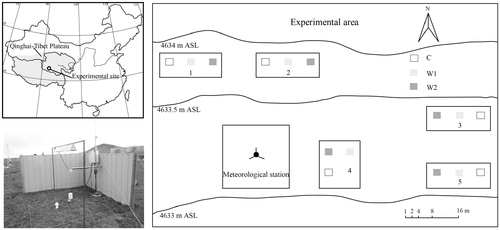
FIGURE 1. Experimental site, design, and plots.

For these reasons, it is extremely important to understand how warming influences water and heat fluxes and their interaction in the QTP for the purpose of predicting the future of alpine ecosystems and providing the regional data needed for AGCM LSMs. An experiment was conducted in the QTP to quantitatively evaluate the impact of experimental warming on heat and water fluxes during the thawed period (July–September 2010 and 2011) in the alpine region. The thawed period was selected as the research period because in the experimental area the soil in the active layer (0–3 m depth) is completely unfrozen during this time. In other months, snow cover has a high albedo and acts as an insulator between the atmosphere and the soil surface, greatly reducing heat and water transfer. Frozen soil may also affect water and heat flux in the soil profile. Heat and water fluxes belowground and near the surface up to 20 cm are the focus of this study because most of the effect of infrared heating is found near the soil surface (Wan et al., 2002; Kimball, 2005; Amthor et al., 2010).

Methodology

SITE DESCRIPTION

The experimental site has an alpine climate and is located in the heart of the QTP with coordinates of 92°55′E and 34°49′N at an altitude of 4635 m a.s.l. (Fig. 1). Based on metrological station data collected from 2008 to 2011, mean annual air temperature is -3.8 °C, mean annual maximum air temperature is 19.2 °C, mean annual minimum air temperature is -27.9 °C, mean air temperature in the growing season (from July to September) is 4.3 °C, mean annual precipitation is 290.9 mm with over 95% falling during the warming season (from April to October), mean annual evaporation is 1316.9 mm, and mean annual relative humidity is 57%. Mean annual wind velocity is 4.1 m s^-1, though maximum wind velocity can exceed 20 m s^-1 in winter and 16 m s^-1 in summer. Soil development is weak, and soils are classified as Mattic Cryic Cambisols (Alpine meadow soil, as Cambisols in FAO/UNESCO taxonomy) with a mattic epipedon at a depth of approximately 0–10 cm and an organic-rich layer at 20–30 cm (Wang et al., 2007). The site is dominated by alpine meadow vegetation, including Kobresia capillifolia, Kobresia pygmaea, Carex moorcroftii, with a mean height of 5 cm.

EXPERIMENT DESIGN

A randomized block design with five replicate blocks was used (Fig. 1). The distances between the blocks ranged from 10 to 50 m. The topography and vegetation in different blocks were different. In each block, there were three 2 × 2 m plots: one control plot, one moderately warmed plot, and one intensely warmed plot. These plots were all at least 4 m apart. Within each block, the three plots were similar in topography, soil texture, aboveground biomass, and species composition. Warmed plots were subjected to continuous warming from 2 July 2010 (and is still ongoing), while control plots (C) were left at ambient temperatures. A single infrared heater (165 × 15 cm, Kalglo Electronics, Bethlehem, Pennsylvania, U.S.A.) was suspended 1.5 m above each warmed plot with a radiation output of 130 W m^-2 in the moderately warmed (W1) plots and of 150 W m^-2 in the intensely warmed (W2) plots. The reflector surfaces of the heaters were adjusted to distribute radiant energy evenly to the soil surface. The control plot had a dummy heater with the same dimensions as the infrared heater suspended at the same height to control for shading effects (Kimball, 2005). In order to reduce the effect of strong winds and to protect the instruments, a 1.5-m-high steel plate was installed on the windward side of each plot (Fig. 1). Wind profiles were simultaneously measured in and out of the plots to evaluate the influence of the steel plate on wind velocity inside the plot. The measured results (Appendix Fig. A1) show that the influence of the wind barrier on wind velocity at the height of 20 cm inside the plot is smaller, which should not affect an experiment focusing on the ground and near ground surfaces.

A micro-meteorological station was set up near the experimental blocks to measure the features of the local microclimate, such as air temperatures and wind speeds at the height of 50, 100, 200, and 400 cm; soil surface temperature; soil temperature at depths of 10, 20, 40, 60, and 100 cm; precipitation; evaporation; net long-wave radiation; net short-wave radiation; photosynthetically active radiation; and ground heat flux (Fig. 1). According to meteorological station records, the mean air temperature at a height of 1 m from July to September was 6.90 °C in 2010 and 5.43 °C in 2011. The precipitation from July to September was 180.1 mm in 2010 and 317.9 mm in 2011.

For better understanding of soil temperature and water, soil samples were taken from depths of 0–10, 10–20, 20–40, 40–70, and 70–100 cm in each plot when instruments were installed. Samples were measured for soil texture by a laser-light diffraction instrument (Arriaga et al., 2006), soil bulk density by the core method (Sala et al., 2000), soil carbon content by the potassium dichromate oxidation titration method (Walkley, 1947), CaCO₃ by the gasometrical method (Schettler, 1968), and pH by acidimeter. There was no significant difference for all these initial soil variables among the three treatments. Table 1 shows the mean values of these measures in 15 plots. In addition, belowground biomass in the experimental site also was measured to help in understanding its influence on heat and water fluxes (Table 2).

MEASUREMENT OF TEMPERATURE AND WATER

Model HMP45C Vaisala Temperature and Relative Humidity Probes (Campbell Scientific, U.S.A.) were installed at a height of 20 cm above the soil surface at the center of each plot to monitor air temperature and relative humidity. 41003-5 Gill Radiation Shields were used to protect sensors of probes from upward or downward direct radiation. SI-111 Apogee 20 Infrared Radiometers (Campbell Scientific, U.S.A.) were hung 80 cm above the ground to monitor soil surface temperature. Four Model 109SS-L Temperature Probes with an endurance range of -40–100 °C (Campbell Scientific, U.S.A.) were installed at a depth of 20, 40, 60, and 100 cm to monitor soil temperatures from 2 July 2010 to 5 October 2011. For better monitoring of the temperature change in the soil surface and the deep ground, new probes were added on 15 October 2011, and the monitor profile was changed to be depths of 5, 15, 30, 60, 100, 150, 200, 250, and 300 cm. All probes were connected to a CR1000 data logger capable of withstanding low temperatures (Campbell Scientific, U.S.A.).

EnviroSMART (Australian Sentek) probes, based on frequency domain reflection (FDR), were installed at depths of 10, 20, 40, 60, and 100 cm in each plot to simultaneously monitor soil volumetric water content across the entire experiment. Before installing probes, absolute calibrations were conducted for each probe. Five replicate samples of soil were first collected 10 cm from the location that the FDR probes were placed. The gravimetric soil water content was obtained by the oven drying method (at 105 °C for 24 hours to achieve a constant weight) then converted to volumetric soil water content by multiplying by the corresponding volume weight of soil. Linear regression analysis (R ² = 0.51) of volumetric soil water content between that measured by FDR and by the oven drying method was constructed to calibrate the FDR probes. Soil water information was collected by a CR1000 data logger installed in each plot.

Air temperatures, air relative humidity, soil surface temperatures, soil temperatures, and soil water contents were automatically collected at 10-minute intervals from 2 July 2010 to the present.

DATA CALCULATION

Gr_{soil tem}, Gr_{soil water}, and ΔT_air-ground

Due to the freezing and thawing processes, which greatly affect soil heat and water fluxes, only the temperature and water changes during the warmest season, July through September (2010–2011), when no freeze or thaw processes occurred in the soil at 0–100 cm depth, were used. The daily (0:00–24:00), day (8:00–19:50), and night (20:00–7:50) mean values for each day from July 2010 to September 2010 and from July 2011 to September 2011 for all observed factors in 15 plots were first obtained. Then, the average daily, day, and night mean temperatures, soil water content, air relative humidity, and vapor pressure for the C, W1, and W2 treatments and their standard deviations during the research period were calculated based on the values from each plot (five replicates per treatment). Based on the average daily, day, and night mean temperatures and soil water content, the soil temperature gradients (Gr _{soil tem}) from the soil surface to 100 cm in depth, soil water content gradients (Gr _{soil water}) from 10 to 20 cm in depth, and soil water content gradients (Gr _{soil water}) from 20 to 100 cm in depth in each plot were calculated by constructing linear regression equations (R ² > 0.94, P < 0.0001).

Different from ground heat fluxes, heat transfers to the atmosphere depend more on convective turbulence resulting from conduction of sensible heat (H) from the surface to the near-surface air. The magnitude of H is determined by the temperature of the soil surface and the near-surface air. We calculated the temperature difference between the soil surface and the near-surface air (ΔT _air-ground) based on the measured temperatures of the soil surface and air at a height of 20 cm in the experimental plots.

TABLE 1 Physical and chemical properties of the soil in the treatment plots (mean ± SD).

G, LE, AND H

Ground heat flux (G) is the conductive heat flux between the soil surface and deeper soils. Its magnitude depends on the thermal gradient between the soil surface and deep soil, which is affected by soil temperature, soil moisture, and soil texture. G _e is ground heat flux in experimental plots and was calculated according to Equation 1 (McCumber and Pielke, 1981). C _1e is the thermal conductivity in the experimental plots and is assumed to be equal to that at the meteorological station, C _1m, because the physical properties of the soil at both sites were similar. ∂̸te/∂̸ze is the Gr_{soil_tem} in experimental plots and can be determined by the above description.

G _m and ∂̸tm/∂̸zm are the G and Gr_{soil_tem} at the meteorological station, respectively, and were directly measured. According to Equation 2, C _1m, therefore can be calculated.

TABLE 2 Distribution pattern of belowground biomass in the experimental site during the warm growing season (mean ± SD).

With C _1m = C _1e, G _e can be determined based on the calculated Gr_{soil_tem} in experimental plots.

Latent heat flux (LE) is the flux of heat from the earth's surface to the atmosphere that is associated with evaporation or transpiration of water from soil or vegetation. Sensible heat flux (H) is the conductive heat flux from the earth's surface to the atmosphere that is associated with ground and air temperature. LE is thought to be most important during the summer when moisture evaporates from the surface and the active layer thaws (Julia et al., 2008). However, LE and H were not calculated in this study because of the lack of observations of temperature and relative humidity from higher layers of air. In addition, the wind barriers produced eddy currents on the leeward side of barriers and affected temperature and vapor pressure in the higher air layers in the plots.

AVP, SVP, AND VPD

The actual vapor pressure (AVP) is the vapor pressure exerted by the water in the air, which can directly reflect the amount of water in the air. In this research, the actual vapor pressure (AVP) is calculated from the measured relative humidity (RH) and the calculated saturation vapor pressure (SVP) by the following equation (Allen et al., 1998): When the air is saturated and cannot store any extra water molecules, the vapor pressure in the air is called the saturation vapor pressure (SVP). Because the number of water molecules that can be stored in the air depends on the temperature, SVP can be calculated by the equation: The vapor pressure deficit (VPD) is the difference between the AVP and the SVP for a given time period, and can be calculated by the equation:

The vapor pressure deficit (VPD) is the difference between the AVP and the SVP for a given time period, and can be calculated by the equation:

STATISTICAL ANALYSIS

One-way ANOVA and post hoc Tukey's multiple comparison tests were used with a significance level of 0.05 to evaluate the statistical significance of warming treatments for temperatures of soil, soil surface and air, soil water, relative humidity, Gr_{soil tem}, Gr_{soil water}, ΔT _air-ground, and G using SPSS 16.0 for Windows.

TABLE 3 Daily, day, and night mean values of environmental factors at different depths under different treatments in July, August, and September of 2010.

Results

RESPONSE OF TEMPERATURES, TEMPERATURE GRADIENTS, AND TEMPERATURE DIFFERENCES

Infrared heating resulted in the daily mean soil surface temperature increasing about 1 °C in the moderately warmed plots (W1) and about 3 °C in the intensely warmed plots (W2). Our results showed that experimental warming had no significant effect on air temperature in either W1 or W2 plots relative to the control plots (Tables 3 and 4, and Fig. 2, parts a and g) during the two years of this experiment. However, infrared heating significantly increased (P < 0.01) soil surface and soil temperature in the warmed plots (Tables 3 and 4, and Fig. 2, parts b–f, h–l). Soil tended to be warmest at the surface, and heater-induced increases in soil temperature decreased as soil depth increased (Figs. 2 and 3; Appendix Fig. A2).

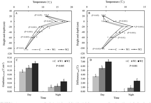
Experimental warming significantly (P < 0.01) increased temperature gradients from the soil surface to a soil depth of 100 cm (Tables 3 and 4 and Fig. 3, part c) and temperature differences between the soil surface and air temperature at a height of 20 cm (Tables 3 and 4 and Fig. 3, part d) for both 2010 and 2011. From Fig. 3, part a, and Tables 3 and 4, it can be seen that soil temperatures decreased from the surface to the depth of 100 cm for all the plots during the day (8:00–19:50). Different from the pattern during day, the soil mean temperature at night (20:00–7:50) first increased from the soil surface to a depth of 20 cm, and then decreased with increasing depths in the control and heated treatments (Fig. 3, part b; Appendix Fig. A3).

FIGURE 2. Daily average temperatures measured at (a and g) 20 cm above the soil surface, (b and h) the soil surface, and depths of (c and i) 20 cm, (d and j) 40 cm, (e and k) 60 cm, and (f and l) 100 cm in the control (dotted line), moderately warmed (W1; solid line), and intensely warmed treatments (W2; dashed line) from July to September, in 2010 and 2011, respectively.

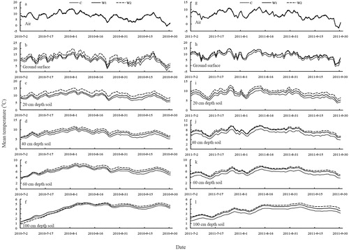
TABLE 4 Daily, day, and night mean values of environmental factors at different depths under different treatments in July, August, and September of 2011.

Experimental warming caused Gr_soil tem to increase by 0.02 °C cm^-1 and 0.04 °C cm^-1 during the day, and by 0.01 °C cm^-1 and 0.03 °C cm^-1 at night in W1 and W2 plots, respectively, in 2010 (Table 3 and Fig. 3, part c). Similar to the pattern in 2010, experimental warming caused Gr _{soil tem} to increase by 0.01 °C cm^-1 and 0.02 °C cm^-1 during the day, and by 0.01 °C cm^-1 and 0.01 °C cm^-1 at night in W1 and W2 plots, respectively, in 2011 (Table 4). In addition, experimental warming also increased ΔT _air-ground by 1.92 °C and 3.47 °C in 2010, 1.71 °C and 1.55 °C in 2011 in W1 and W2 plots, respectively, during the day, and by 0.79 °C and 2.42 °C in 2010, and 0.99 °C and 1.38 °C in 2011 in W1 and W2 plots, respectively, during the night (Tables 3 and 4). The influences of experimental warming on Gr_{soil tem} and ΔT _air-ground during the day are higher than those during the night (Figs. 3, parts c and d).

FIGURE 3. Average temperatures profiles during (a) day and (b) night. (c) Soil temperature gradients from 100 cm in depth to the soil surface (0 cm) during day and night. (d) Air temperature differences between the soil surface (0 cm) and 20 cm in height during day and night from 2 July to 30 September 2010. Control treatments are indicated by the dotted line or the light gray bar, moderately warmed (W1) treatments are indicated by the dashed line or the gray bar, and intensely warmed (W2) treatments are indicated by the solid line or the black bar. Different letters indicate statistically significant differences at the corresponding confidence interval among the three treatments as determined by ANOVA followed by a Tukey test. Error bars represent the standard error for n = 5.

RESPONSE OF SOIL LIQUID WATER CONTENT AND SOIL LIQUID WATER CONTENT GRADIENTS

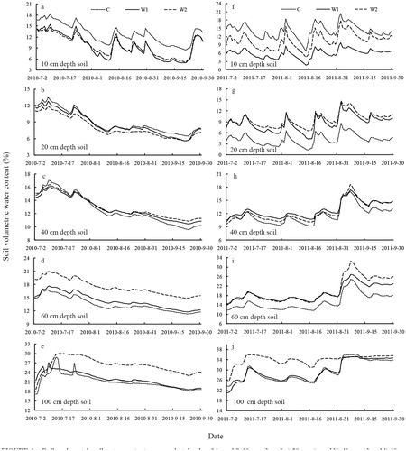
There was no significant difference in the soil liquid water content between day and night, and the same pattern was observed at both day and night in the experiment. Soil liquid water content first significantly (P < 0.001) decreased with increasing depth from 10 to 20 cm, and significantly increased with increasing depth from 40 to 100 cm both in 2010 and 2011 (Tables 3 and 4, Figs. 4 and 5). The influence of experimental warming gradually weakened from 20 to 40 cm in depth with no significant change.

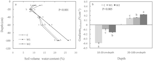
Gr_{soil water} in the profile from 10 to 20 cm in depth was negative because soil water content decreased as the depths increased (Fig. 5, part b). Experimental warming alleviated the decreasing effect and significantly (P < 0.005) decreased Gr_{soil water} by 0.30% cm^-1 and 0.23% cm^-1 in 2010, 0.23% cm^-1 and 0.24% cm^-1 in 2011, in the profile from 10 to 20 cm in depth in W1 and W2 plots, respectively (Fig. 5, parts a and b). In the profile from 20 to 100 cm in depth, experimental warming significantly (P < 0.005) increased Gr_soil water by 0.08% cm^-1 and 0.01% cm^-1 in 2010, 0.02% cm^-1 and 0.05% cm^-1 in 2011 in W1 and W2 plots, respectively.

FIGURE 4. Daily volumetric soil water content measured at depths of (a and f) 10 cm, (b and g) 20 cm, (c and h) 40 cm, (d and i) 60 cm, and (e and j) 100 cm in the control (dotted line), moderately warmed (W1; solid line), and intensely warmed treatments (W2; dashed line) from July to September, in 2010 and 2011, respectively.

RELATIVE HUMIDITY AND VAPOR PRESSURE

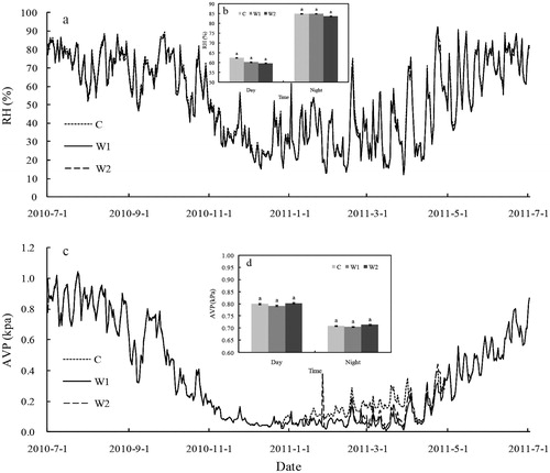
Along with the liquid water in the soil, we also examined the vapor phase water in the atmosphere for a better understanding of the water flux process. In both 2010 and 2011, there were no significant differences among the different treatments in the mean air relative humidity and actual vapor pressure at a height of 20 cm above the soil surface (Table 3, Fig. 6). The change in relative humidity caused by warming showed the same pattern during day and night. Also, compared to the control plots, the vapor pressure deficit (VPD), non-significantly increased by 0.03 kpa in the W2 treatment and 0.01 kpa in the W1 treatment in 2010. The pattern in 2011 is the same (Table 4). In contrast to the non-significant change in saturation vapor pressure of air at 20 cm above the soil surface, the saturation vapor pressure in the plant canopy significantly (P < 0.001) increased by 0.42 kpa and 0.81 kpa in the W1 and W2 plots, respectively, in 2010 and by 0.42 kpa and 0.48 kpa in the W1 and W2 plots, respectively, in 2011.

FIGURE 5. (a) Average volumetric soil water content profile at depths from 10 to 100 cm and (b) volumetric soil water content gradients from 10 to 20 cm in depth and from 20 to 100 cm in depth from 2 July to 30 September 2010 in the control (dotted line or light gray bar), moderately warmed (W1; dashed line or gray bar), and intensely warmed treatments (W2; solid line or black bar). Different letters indicate statistically significant differences at P < 0.05 among the three treatments, as determined by ANOVA followed by Tukey's test. Error bars represent the standard error for n = 5.

GROUND HEAT FLUX

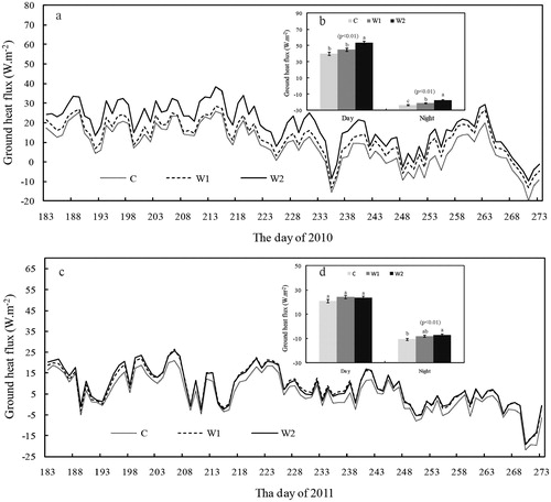
Infrared heating significantly (P < 0.001) increased daily mean value of G by 9.76 W m^-2 in the W2 treatment and 3.67 W m^-2 in the W1 treatment in the growing season of 2010 (Fig. 7, part a). During the day, G is positive and heat in the soil surface is conducted down into the soil. Infrared heating significantly (P < 0.01) increased G during the day by 13.46 W m^-2 in the W2 treatment and nonsignificantly (P > 0.05) increased G during the day by 4.76 W m^-2 in the W1 treatment. At night, G is negligible and heat is conducted back up to surface. Infrared heating significantly (P < 0.01) increased G at night by 6.02 W m^-2 in the W2 treatment and 2.37 W m^-2 in the W1 treatment (Fig. 7, part b). The same pattern can be found during the growing season of 2011, but with increased values and reduced significance (Fig. 7, part c). Infrared heating significantly (P < 0.05) increased daily mean value of G by 3.19 W m^-2 in the W2 treatment and by 3.00 W m^-2 in the W1 treatment. During the day, the increase is nonsignificant. At night, warming significantly (P < 0.05) increased G by 3.57 W m^-2 in the W2 treatment (Fig. 7, part d).

Discussion

RESPONSE OF HEAT FLUX TO EXPERIMENTAL WARMING

In most ecosystems, heat is conducted down into the soil during the day and back up to the surface at night (Chapin et al., 2011). Our observed results in both control and warmed plots show that the air and soil surface temperatures exhibited diurnal variance, especially on the soil surface, while soil temperatures deeper than 20 cm remained stable during the day and night. During the day, solar shortwave radiation directly heats the soil surface, which results in soil surface temperatures reaching 15–20 °C, which is higher than that of air and soil in 20 cm depth, which are both 10 °C during the day. At night, the soil surface and air temperatures rapidly decreased to about 5 °C, while the soil temperature remained at 10 °C. The great variance in the daily soil surface temperature probably comes from two reasons. The first reason is the study area's thinner atmosphere and clear sky at an elevation of 4600 m a.s.l., resulting in a high proportion of the incoming solar shortwave radiation reaching the soil surface and heating the soil surface during the day; the energy absorbed by the soil during the day is again released back to the atmosphere at night. The other reason is related to the low soil thermal capacity of sandy soils. In the experimental area, sandy soil with a particle size of above 0.02 mm makes up about 96-98% of the total soil at depths of 0–50 cm (Table 1). Sandy soils usually have a low soil thermal capacity and high soil heat conductance, which can induce great diurnal temperature fluctuations. Using an infrared heater, Luo et al. (2010) also found that manipulative warming induced a higher increase of soil temperature during the day than that at night, and the soil temperature difference between day and night decreased from the depth of 5 cm to10 cm in the northeast Qinghai-Tibet Plateau.

The magnitude of ground heat flux depends on the thermal gradient between the soil surface and the deep soil. The great variance in daily surface temperature resulted in an increasing soil temperature gradient between the soil surface and deep soils in the control plots, which resulted in greater heat conduction and energy transfer. Experimental warming did not change in pattern from the control treatments, but significantly increased soil surface and soil temperatures, together with soil temperature gradients and temperature differences between the surface and near-surface air, which is consistent with that reported in the other regions including temperate tallgrass prairie and alpine meadow (Harte et al., 1995; Bridgham et al., 1999; Wan et al., 2002; Saleska et al., 2002; Luo et al., 2010). Experimental warming caused steep thermal gradients, which further encouraged the ground heat flux between the deep soil and the soil surface. In contrast to the ground heat flux, heat transferring to the atmosphere depends more on convective turbulence resulting from the conduction of sensible heat from the surface to the near-surface air. The temperature of the surface and near-surface air determines the magnitude of sensible heat. Experimental warming resulted in higher temperature differences between the surface and near-surface air which likely increased the sensible heat transfer. Compared to soil temperature gradients and temperature differences between the day and night, experimental warming caused greater effects on ground heat flux and sensible heat during the day than during the night.

FIGURE 6. (a) Daily relative air humidity, (b) average relative air humidity, (c) daily actual vapor pressure, and (d) actual vapor pressure at a height of 20 cm from 2 July to 30 September 2010 in the control (dotted line and light gray bar), moderately warmed (W1; solid line and gray bar), and intensely warmed treatments (W2; dashed line and black bar). The same letters indicate statistically insignificant differences at P < 0.05 among the three treatments, as determined by ANOVA. Error bars represent the standard error for n = 5.

It should be noted that although experimental warming caused soil temperatures, soil temperature gradients, and temperature differences to significantly increase, the air temperature near the surface did not significantly increase. This is consistent with results from a montane meadow near the Rocky Mountain Biological Laboratory (RMBL), with the same type of warming facility (Saleska et al., 2002). In that study, warming meadow heaters had negligible effects on air temperature above plots. In tallgrass prairie of Oklahoma, heater-induced warming also had no significant effect on daily maximum air temperature (Wan et al., 2002). The response of daily mean and minimum air temperatures at the height of 20 cm was significant and higher than these measures in our experiment, although infrared heaters used in our experiment added additional radiation of 130 and 150 watts m^-2 in W1 and W2 plots, respectively, which are higher than those used in the tallgrass prairie of Oklahoma, with a radiation output of 100 watts m^-2. The difference is speculated to be due to the fact that the average plant canopy height in Oklahoma exceeded 50 cm and air temperature measured in a warming experiment should be affected by a canopy due to its high heat absorption rate. In our experimental plots, the average plant canopy height was 5 cm and air temperature probes were installed at a height of 20 cm above the ground. The measured air temperatures in our experimental plots should be the air temperature without effects from plants. In addition, this nonsignificant increase of air temperature was attributed to slow soil conductivity and mechanical turbulence from horizontal airflow moving across near the surface (the average wind velocity near the surface exceeded 2 m s^-1 and the average maximum wind velocity near the surface exceeded 8 m s^-1 during the warm season).

FIGURE 7. Daily ground heat flux from 2 July to 30 September in the control (dotted line), moderately warmed (W1; dashed line), and intensely warmed treatments (W2; solid line) in (a) 2010 and (c) 2011. Average ground heat flux during day and night from 2 July to 30 September in the control (light gray bar), moderately warmed (W1; gray bar), and intensely warmed treatments (W2; black bar) in (b) 2010 and (d) 2011. Different letters indicate statistical significance at P < 0.05 among the three treatments, as determined by ANOVA. Error bars represent the standard error for n = 5.

RESPONSE OF SOIL WATER FLUX TO EXPERIMENTAL WARMING

The water-holding capacity of the soil in the experimental area is low due to the high proportion of sand in the soil (Table 1). The volumetric soil water content in both control and warmed plots increased from 7% in 20 cm in depth to 20–25% at 100 cm in depth. Increasing soil water content with depth likely comes from the downward water movement under the force of gravity due to the low water-holding capacity of coarse-textured sandy soils. Different from the increasing trend of the water content in the deep soil layer, the soil water content in the shallow layer gradually decreased from 10 to 20 cm in depth. The pattern of the shallow soil water content was attributed to the mattic epipedon and soil organic matter. In the experimental area, the soil with thick mattic epipedon (mainly consisting of dead roots) and organic matter, mainly distributed in depths of 0–20 cm (Table 2), could hold more water than deep coarse sandy soil and therefore is beneficial to soil water storage.

Experimental warming significantly decreased the soil water content in the shallow layer. The hydrologic cycle in the ecosystem is driven by energy transfer; soil surface evaporation and plant transpiration always accompany heat transfer from the soil to the atmosphere. Increased soil surface temperatures and temperature gradients between the soil surface and the atmosphere resulting from experimental warming likely accelerated the process of latent heat in addition to ground heat flux and sensible heat, which may cause the corresponding evaporation of soil water. On the other hand, plant roots were mostly distributed in the upper soil layer (0–20 cm) in the study area (Table 2). Experimental warming may stimulate plant growth, which causes water to move from soil to the roots of transpiring plants. This is another possible cause of the decrease in soil water in the shallow layer in the warming treatments.

The study area is located in an area with continuous permafrost and the thickest active layer in China. Permafrost is soil that remains at or below 0 °C for two or more years, and its thickness can vary from a few centimeters to several hundreds of meters. Overlying the permafrost is the active layer, which is typically 0.5–4 m thick. The active layer thaws during the summer and refreezes during the autumn. The thickness of the active layer ranged from 2.0 to 3.2 m in our experiment site (Lu et al., 2006; Pang et al., 2009). The thickness of the active layer has increased by 3.1 cm per year since the 1980s due to global warming (Wu and Liu, 2004). Heating also enhanced the thawing process in the active layer during the warming season. The experiment results showed that increased soil temperature from intense warming reduced the frozen thickness in the active layer by 2–20 cm and increased the thaw thickness in the active layer by 10–40 cm, and shortened the duration of the seasonal freeze in the active layer by 9–30 days (unpublished data). The increased thaw duration and the active layer thickness increased soil water content. This water was then pulled downward by gravity. Experimental warming resulted in soil water increases with increasing depths lower than a depth of 20 cm. This is consistent with the results published by Yang et al. (2003), whose study was performed along the Qinghai-Tibetan highway. At the same time, experimental warming also increased water content gradients deeper than 20 cm, which accelerates water moving down because of increasing differences in water potentials, causing soil water content to increase with depth.

RESPONSE OF ATMOSPHERIC VAPOR WATER FLUX TO EXPERIMENTAL WARMING

Some reports point out that an experimental increase of air temperature will cause a drop in relative humidity if the humidity is not controlled (Amthor et al., 2010). However, global warming is expected to cause the absolute humidity of the air to increase, while relative humidity remains more or less constant (IPCC, 2001, 2007). Therefore, Kimball (2005, 2011) proposed that an ideal experimental system should both heat the air and humidify it to maintain constant relative humidity; for example, drip irrigation is recommended to control the relative humidity.

No significant change in atmospheric relative humidity and vapor pressure at a height of 20 cm was found in the warmed plots compared to the control plots in our study, which is consistent with the atmospheric relative humidity pattern predicted by some models (IPCC, 2007). It is speculated that nonsignificant increase of air temperatures resulted in the nonsignificant decrease of atmospheric relative humidity. In addition, the thaw of frozen soil caused by warming releases some water vapor into the atmosphere and can compensate for the reduction of relative humidity. In our warming experimental plots, vegetation is short with an average height of 5 cm. The soil surface temperatures measured by infrared radiometers are also the plant canopy temperatures. The calculated saturation vapor pressure in the plant canopy based on the maximum and minimum canopy temperatures significantly increased in the warmed plots compared to the control plots. When actual vapor pressure stays stable, the relative humidity will significantly decrease in the canopy. Since warming had not caused significant change in the saturation vapor pressure in air, the vapor pressure gradients (VPGs) from inside the canopy to the air will increase, which possibly caused the inconsistency of the atmospheric vapor fluxes in the experiment compared to the global warming pattern. Therefore, a first-order correction to the VPG problem recommended by Kimball (2005) should be considered in the future experimental designs in order to achieve better parameterization of the related factors used in AGCMs and to predict global warming more accurately.

Conclusions

High quality and quantity knowledge of the probable responses of terrestrial ecosystems to global warming is very important in order to use in the correct parameterization during construction of AGCM LSMs and to precisely predict the development of terrestrial ecosystems in the future. Using infrared heating, the effects of experimental warming on heat and water fluxes of soil and the soil surface were studied in alpine meadows with permafrost in the central region of the QTP. Although the mechanism of infrared heating of soil and plants is different from global-warming—induced soil and plant warming by warmer air, heat and water flux change from infrared heating still can effectively reflect actual energy fluxes under elevated soil and plant temperatures and thereby provides data for use in the parameterization of related factors for the AGCM LSMs.

In our study, when 130 and 150 W m^-2 of infrared radiation from a height of 1.5 m were used in the plots, the soil and soil surface temperatures significantly increased, accompanied by the nonsignificant increase of air temperature. The influences of experimental warming on soil temperature gradients and temperature differences during the day are higher than those during the night. Accordingly, significantly increased ground heat fluxes can accelerate the heat transfer process between the soil and the soil surface. Driven by the accelerated heat flux, the movement of the water inside the soil and between the soil and the atmosphere also changed. An important change was the decrease of soil water content in the shallow soil layer and the soil surface, which can cause the soil surface to dry. However, 2 years of experimental warming did not cause a significant change in atmospheric relative humidity and vapor pressure, although a trend of decreasing relative humidity was observed. Therefore, we think the response of heat and water fluxes in soil to warming is quicker and larger than that in the atmosphere, which can directly influence the development of alpine ecosystems.

Acknowledgments

This research was financially supported by the “One Hundred Talents Program” of the Chinese Academy of Sciences. The authors would like to thank professor Yongzhi Liu and all the staff at Beiluhe Station for their kind assistance in the field and for providing the experimental site. The authors also would like to thank four reviewers and editors for their valuable suggestions and comments.

FIGURE A1. The relation of wind velocities between inside and outside of the plot at the height of (a) 20 cm, (b) 50 cm, (c) 100 cm, and (d) 200 cm above the ground surface.

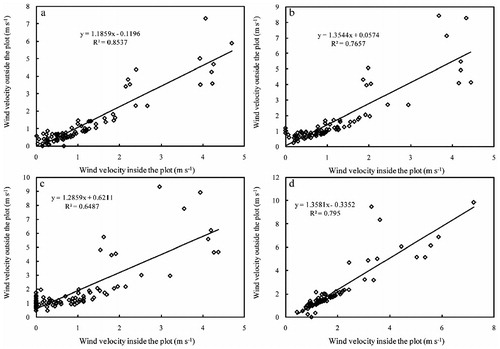
FIGURE A2. Daily average temperatures measured at (a) 20 cm above the soil surface, (b) at the soil surface, and at depths of (c) 20 cm, (d) 40 cm, (e) 60 cm, and (f) 100 cm in the control (dotted line), moderately warmed (W1; solid line), and intensely warmed treatments (W2; dashed line) from 2 July 2010 to 1 July 2011.

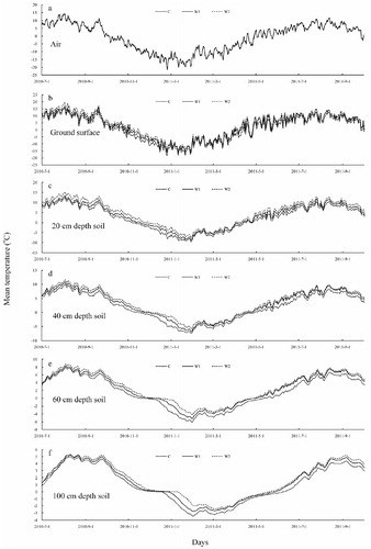
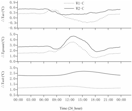
FIGURE A3. Anomalies (compared to the control plot) of annual averages of hourly (a) air, (b) ground surface, (c) 20 cm, and (d) 100 cm underground temperatures for (W1-C) moderately warmed plots and (W2-C) intensely warmed plots during 2 July 2010 to 1 July 2011. W1-C shows values equal to those of moderately warmed plots minus the values in control plots; W2-C shows values equal to those of intensely warmed plots minus the values in control plots.

References Cited

- ACIA , 2004: Arctic Climate Impact Assessment: Scientific Report. Cambridge: Cambridge University Press, 144 pp.
- Allen, R. G. , Pereira, L. S. , Raes, D. , and Smith, M. , 1998: Crop evapotranspiration-Guidelines for computing crop water requirements. Rome: FAO, Irrigation and Drainage Paper No. 56, 300 pp.
- Amthor, J. S. , Hanson, P. J. , Norby, R. J. , and Wullschleger, S. T. , 2010: A comment on “Appropriate experimental ecosystem warming methods by ecosystem, objective, and practicality” by Aronson and McNulty. Agricultural and Forest Meteorology , 150: 497–498.
- Aronson, E. L. , and McNulty, S. G. , 2009: Appropriate experimental ecosystem warming methods by ecosystem, objective, and practicality. Agricultural and Forest Meteorology , 149: 1791–1799, doi: <http://dx.doi.org/10.1016/j.agrformet.2009.06.007>.
- Arriaga, F. J. , Lowery, B. , and Days, M. D. , 2006: A fast method for determining soil particle size distribution using a laser instrument. Soil Science , 171: 663–674.
- Baldocchi, D. D. , 2003: Assessing the eddy covariance technique for evaluating carbon dioxide exchange rates of ecosystems: past, present, and future. Global Change Biology , 9: 479–492.
- Bridgham, S. D. , Pastor, J. , Updegraff, K. , Malterer, T. J. , Johnson, K. , Harth, C. , and Chen, J. , 1999: Ecosystem control over temperature and energy flux in northern peatlands. Ecological Applications , 9:1345–1358.
- Brown, J. , Hinkel, K. M. , and Nelson, F. E. , 2000: The Circumpolar Active Layer Monitoring (CALM) program: research designs and initial results. Polar Geography , 24: 165–258.
- Chapin, F. S., III , and Shaver, G. R. , 1985: Individualistic growth response of tundra plant species to environmental manipulation in the field. Ecology 66: 564–576.
- Chapin, F. S. , III, Matson, P. A. , and Vitousek, P. M. , 2011: Principles of Terrestrial Ecosystem Ecology. 2nd edition. New York: Springer.
- Chen, T. H. , Henderson-Sellers, A. , Milly, P. C. D. , Pitman, A. J. , Beljaars, A. C. M. , Abramopoulos, F. , Boone, A. , Chang, S. , Chen, F. , Dai, Y. , Desborough, C. E. , Dickinson, R. E. , Dümenil, L. , Ek, M. , Garratt, J. R. , Gedney, N. , Gusev, Y. M. , Kim, J. , Koster, R. D. , Kowalczyk, E. , Laval, K. , Lean, J. , Lettenmaier, D. P. , Liang, X. , Mengelkamp, T.-H. , Mahfouf, J.-F. , Mitchell, K. , Nasonova, O. , Noilhan, J. , Polcher, J. , Robock, A. , Rosenzweig, C. , Schaake, J. C. , Schlosser, C. A. , Schulz, J.-P. , Shao, Y. , Shmakin, A. B. , Verseghy, D. L. , Wetzel, P. , Wood, E. F. , Xue, Y. , Yang, Z.-L. , and Zeng, Q. , 1997: Cabauw experimental results from the Project for Intercomparison of Land-Surface Parameterization Schemes (PILPS). Journal of Climate , 10: 1194–1215.
- Cheng, G. D. , Huang, X. , and Kang, X. , 1993: Recent permafrost degradation along the Qinghai-Tibet Highway. In Permafrost Sixth International Conference Proceedings. Vol. 2. Wushan, Guangzhou, China: South China University of Technology Press, 1010–1013.
- Cornwell, A. R. , and Harvey, L. D. D. , 2008: Simulating AOGCM soil moisture using an off-line Thornthwaite potential evapotranspiration-based land surface scheme. Part I: control runs. Journal of Climate , 21: 3097–3117, doi: <http://dx.doi.org/10.1175/2007JCLI1675.1>.
- Eagleson, P. S. , 2002: Ecohydrology. Darwinian Expression of Vegetation Form and Function. Cambridge: Cambridge University Press, 443 pp.
- Giorgi, F. , Hewitson, B. , and Christensen, J. , 2001: Climate change 2001: regional climate information-Evaluation and projections. In Climate Change 2001: The Scientific Basis. Contribution of Working Group I to the Third Assessment Report of the Intergovernmental Panel on Climate Change , edited by J. T. Houghton , et al. Cambridge: Cambridge University Press, 584–636.
- Harte, J. , Torn, M. S. , Chang, F. R. , Feifarek, B. , Kinzig, A. P. , Shaw, R. , and Shen, K. , 1995: Global warming and soil microclimate: results from a meadow-warming experiment. Ecological Applications, 5: 132–150.
- Hartley, A. E. , Neill, C. , Melillo, J. M. , Crabtree, R. , and Bowles, F. P. , 1999: Plant performance and soil nitrogen mineralization in response to simulated climate change in subarctic dwarf shrub heath. Oikos , 86: 331–343.
- Henderson-Sellers, A. , McGuffie, K. and Pitman, A. J. , 1996: The project for intercomparison of land-surface parameterizations schemes (PILPS): 1992 to 1995. Climate Dynamics , 12: 849–859.
- Henderson-Sellers, A. , Irannejad, P. , McGuffie, K. , and Pitman, A. J. , 2003: Predicting land-surface climates-Better skill or moving targets? Geophysical Research Letters , 30: 1777, doi: <http://dx.doi.org/10.1029/2003GL017387>.
- Hinkel, K. M. , and Nelson, F. E. , 2003: Spatial and temporal patterns of active layer thickness at Circumpolar Active Layer Monitoring (CALM) sites in northern Alaska, 1995–2000. Journal of Geophysical Research , 108(D2): 8168, doi: <http://dx.doi.org/10.1029/2001JD000927>.
- Hobbie, S. E. , and Chapin, F. S., III , 1998: The response of tundra plant biomass, aboveground production, nitrogen, and CO2 flux to experimental warming. Ecology , 79(5): 1526–1544.
- Hollister, R. D. , Webber, P. J. , Nelson, F. E. , and Tweedie, C. E. , 2006: Soil thaw and temperature response to air warming varies by plant community: results from an open-top chamber experiment in northern Alaska. Arctic, Antarctic, and Alpine Research , 38(2): 206–215.
- IPCC , 2001: Climate Change 2001: Synthesis Report. Cambridge: Cambridge University Press.
- IPCC , 2007: Climate Change 2007: the Physical Science Basis. Contribution of Working Group I to the Fourth Assessment Report of the Intergovernmental Panel on Climate Change. Solomon, S. , Qin, D. , Manning, M. , Chen, Z. , Marquis, M. , Averyt, K. B. , Tignor, M. , and Miller, H. L. (eds.). Cambridge: Cambridge University Press, 996 pp.
- Irannejad, P. , Henderson-Sellers, A. , Phillips, T. J. , and McGuffie, K. , 2001: Sensitivity of climate simulations to land surface complexity: beginning AMIP II Diagnostic Subproject 12. In 12th Symposium on Global Change and Climate Variations. Albuquerque, New Mexico: American Meteorological Society, 193–196.
- Jonasson, S. , Havström, M. , Jensen, M. , and Callaghan, T. V. , 1993: In situ mineralization of nitrogen and phosphorus of arctic soils after perturbations simulating climate change. Oecologia , 95(2): 179–186.
- Julia, B. , Birgit, H. , and Kurt, R. , 2008: Heat and water transfer processes in permafrost-affected soils: a review of field and modeling-based studies for the Arctic and Antarctic. In Kane, D. L. , and Hinkel, K. M. (eds.), Ninth International Conference on Permafrost Proceedings. University of Alaska Fairbanks, 149–154.
- Kattenberg, A. , Giorgi, F. , Grassl, H. , Meehl, G. A. , Mitchell, J. F. B. , Stouffer, R. J. , Tokioka, T. , Weaver, A. J. , and Wigley, T. M. L. , 1996: Climate models-Projections of future climate. In Houghton, J. T. , Filho, L. G. M. , Callander, B. A. et al. (eds.), Climate Change 1995: the Science of Climate Change. Cambridge: Cambridge University Press, 285–357.
- Kimball, B. A. , 2005: Theory and performance of an infrared heater for ecosystem warming. Global Change Biology , 11: 2041–2056, doi: <http://dx.doi.org/10.1111/j.1365-2486.2005.1028.x>.
- Kimball, B. A. , 2011: Comment on the comment by Author et al. on “Appropriate experimental ecosystem warming methods” by Aronson and McNulty. Agricultural and Forest Meteorology , 151: 420–424.
- Klein, J. A. , Harte, J. , and Zhao, X. Q. , 2005: Dynamic and complex microclimate responses to warming and grazing manipulations. Global Change Biology , 11: 1440–1451, doi: <http://dx.doi.org/10.1111/j.1365-2486.2005.00994.x>.
- Li, W. H. , and Zhou, X. M. , 1998: Ecosystems of Qinghai-Xizang (Tibetan) Plateau and Approach for Their Sustainable Management. Guangzhou, China: Guangdong Science & Technology Press.
- Li, N. , Wang, G. X. , Yang, Y. , Gao, Y. H. , and Liu, G. S. , 2011: Plant production, and carbon and nitrogen source pools, are strongly intensified by experimental warming in alpine ecosystems in the Qinghai-Tibet Plateau. Soil Biology & Biochemistry , 43: 942–953, doi: <http://dx.doi.org/10.1016/j.soilbio.2011.01.009>.
- Lu, Z. J. , Wu, Q. B. , Yu, S. , and Zhang, L. X. , 2006: Heat and water difference of active layers beneath different surface conditions near Beiluhe in Qinghai-Xizang Plateau. Journal of Glaciology and Geocryology , 28(5): 642–647 (in Chinese).
- Luo, Y. Q. , Sherry, R. , Zhou, X. H. , and Wang, S. Q. , 2009: Terrestrial carbon-cycle feedback to climate warming: experimental evidence on plant regulation and impacts of biofuel feedstock harvest. GCB-Bioenergy , 1(1): 62–74.
- Luo, C. Y. , Xu, G. P. , Chao, Z. G. , Wang, S. P. , Lin, X. W et al., 2010: Effect of warming and grazing on litter mass loss and temperature sensitivity of litter and dung mass loss on the Tibetan Plateau. Global Change Biology , 16: 1606–1617, doi: <http://dx.doi.org/10.1111/j.1365-2486.2009.02026.x>.
- Marion, G. M. , Bockheim, J. G. , and Brown, J. , 1997: Arctic soils and the ITEX experiment. Global Change Biology, 3(Suppl. 1): 33–43.
- McCumber, M. C. , and Pielke, R. A. , 1981: Simulation of the effects of surface fluxes of heat and moisture in a mesoscale numerical model 1. Soil layer. Journal of Geophysical Research , 86: 9928–9938.
- Mearns, L. O. , Easterling, W. , Hays, C. , and Marx, D. , 2001: Comparison of agricultural impacts of climate change calculated from high and low resolution climate change scenarios: part I. The uncertainty due to spatial scale. Climate Change , 51: 131–172.
- Nelson, F. E. , Hinkel, K. M. , Shiklomanov, N. I. , Mueller, G. R. , Miller, L. L. , and Walker, D. A. , 1998: Active-layer thickness in north-central Alaska: systematic sampling, scale, and spatial auto correlation. Journal of Geophysical Research , 10: 28963–28973.
- Nixon, M. , Tarnocai, C. , and Kutny, L. , 2003: Long-term active layer monitoring: Mackenzie Valley, northwest Canada, In Phillips, M. , Springman, S. M. , and Arenson, L. U. (eds.), Permafrost. Vol. 2. Lisse, Netherlands: Swets & Zeitlinger, 821–826.
- Pang, Q. Q. , Cheng, G. D. , Li, S. X. , and Zhang, W. G. , 2009: Active layer thickness calculation over the Qinghai-Tibet Plateau. Cold Regions Science and Technology , 57: 23–28, doi: <http://dx.doi.org/10.1016/j.coldregions.2009.01.005>.
- Pitman, A. J. , Henderson-Sellers, A. , Abramopoulos, F. , Avissar, R. , Bonan, G. B. , Boone, A. , Cogley, J. G. , Dickinson, R. E. , Ek, M. , Entekhabi, D. , Famiglietti, J. , Garrat, J. R. , Frech, M. , Hahmann, A. N. , Koster, R. D. , Kowalczyk, E. , Laval, K. , Lean, L. , Lee, T. J. , Lettenmaier, D. P. , Liang, X. , Mahfouf, J.-F. , Mahrt, L. , Milly, C. , Mitchell, K. , de Noblet, N. , Noilhan, J. , Pan, H. , Pielke, R. , Robock, A. , Rosenzweig, C. , Running, S. W. , Schlosser, C. A. , Scott, R. , Suarez, M. J. , Thompson, S. L. , Verseghy, D. L. , Wetzel, P. , Wood, E. F. , Xue, Y. , Yang, Z.-L. , and Zang, L. , 1993: Results from the Off-line Control Simulation Phase of the Project for Intercomparison of Land-Surface Parameterisation Schemes (PILPS). Columbia, Maryland: GEWEX, IGPO Publication Series Technical Note 7.
- Qin, J. , Yang, K. , Liang, S. L. , and Guo, X. F. , 2009: The altitudinal dependence of recent rapid warming over the Tibetan Plateau. Climatic Change , 97: 321–327.
- Rowell, D. , and Jones, R. , 2006: Causes and uncertainty of future summer drying over Europe. Climate Dynamics , 27: 281–299.
- Sala, O. E. , Jackson, R. B. , Mooney, H. A. , and Howarth, R. W. , 2000: Methods in Ecosystem Science. New York: Springer, 421 pp.
- Saleska, S. R. , Shaw, M. R. , and Fischer, M. L. , 2002: Plant community composition mediates both large transient decline and predicted long-term recovery of soil carbon under climate warming. Global Biogeochemical Cycles , 16: 1055, doi: <http://dx.doi.org/10.1029/2001GB001573>.
- Schaefer, K. , Zhang, T. G. , Bruhwiler, L. , and Barreti, A. P. , 2011: Amount and timing of permafrost carbon release in response to climate warming. Tellus , 63B: 165–180, doi: <http://dx.doi.org/10.1111/j.1600-0889.2011.00527.x>.
- Schettler, H. , 1968: Continuous gasometric carbonate determinations in cuttings from drill holes. In Müller, G. , and Friedman, G. (eds.), Recent Developments in Carbonate Sedimentology in Central Europe. Berlin, Heidelberg: Springer, 254–255.
- Seneviratne, S. , Lüthi, D. , Litschi, M. , and Schär, C. , 2006: Land-atmosphere coupling and climate change in Europe. Nature , 443: 205–209.
- Shao, Y. , and Henderson-Sellers, A. , 1996: Modeling soil moisture: a project for intercomparison of land surface parameterization schemes phase 2(b). Journal of Geophysical Research , 101D: 7227–7250.
- Taylor, H. M. , Jordan, W. R. , and Sinclair, T. R. (eds.), 1983: Limitations to Efficient Water Use in Crop Production. Madison, Wisconsin: American Society of Agronomy, Crop Science Society of America, Soil Science Society of America, 538 pp.
- Walkley, A. , 1947: A critical examination of a rapid method for determining organic carbon in soils-Effect of variations in digestion conditions and of inorganic soil constituents. Soil Science , 63: 251–264.
- Wan, S. , Luo, Y. , and Wallace, L. L. , 2002: Change in microclimate induced by experimental warming and clipping in tallgrass prairie. Global Change Biology , 8: 754–768.
- Wang, G. X. , Wang, Y. B. , Li, Y. S. , and Cheng, H. Y. , 2007: Influences of alpine ecosystem responses to climatic change on soil properties on the Qinghai-Tibet Plateau, China, Catena , 70: 506–514, doi: <http://dx.doi.org/10.1016/j.catena.2007.01.001>.
- Wu, Q. B. , and Liu, Y. Z. , 2004: Ground temperature monitoring and its recent change in Qinghai-Tibet Plateau. Cold Regions Science and Technology , 38: 85–92, doi: <http://dx.doi.org/10.1016/S0165-232X(03)00064-8>.
- Xiao, J. F. , Zhuang, Q. L. , Law, B. E. , et al. 2011: Assessing net ecosystem carbon exchange of U.S. terrestrial ecosystems by integrating eddy covariance flux measurements and satellite observations. Agricultural and Forest meteorology 151: 60–69.
- Yanai, M. , and Wu, G. X. , 2006: Effects of the Tibetan Plateau. In Wang, B. (ed.), The Asian Monsoon. Heidelberg: Springer, 513–549.
- Yang, M. X. , Yao, T. D. , Gou, X. H. , Koike, T. , and He, Y. , 2003: The soil moisture distribution, thawing-freezing processes and their effects on the seasonal transition on the Qinghai-Xizang (Tibetan) Plateau. Journal of Asian Earth Sciences , 21(5): 457–465, doi: <http://dx.doi.org/10.1016/S1367-9120(02)00069-X>.
- Yang, Y. H. , Fang, J. Y. , Tang, Y. H. , Ji, C. J. , Zheng, C. Y. , He, J. S. , and Zhu, B. , 2008: Storage, patterns and controls of soil organic carbon in the Tibetan grasslands. Global Change Biology , 14: 1592–1599, doi: <http://dx.doi.org10.1111/j.1365-2486.2008.01591.x>.
- Yang, M. X. , Nelson, F. E. , Shiklomanov, N. I. , Guo, D. L. , and Wan, G. N. , 2010: Permafrost degradation and its environmental effects on the Tibetan Plateau: a review of recent research. Earth-Science Reviews , 103: 31–44.
- Zhao, L. , Ping, C. L. , Yang, D. Q. , Cheng, G. D. , Ding, Y. J. , and Liu, S. Y. , 2004: Changes of climate and seasonally frozen ground over the past 30 years in Qinghai-Xizang (Tibetan) Plateau, China. Global and Planetary Change , 43: 19–31.