Measuring and Modeling the Retreat of the Summit Ice Fields on Kilimanjaro, East Africa

Abstract

Terrestrial laser-scanning surveys of the south-facing cliff of the northern Ice Field on the summit crater of Kilimanjaro were taken on three occasions, in September 2004, January 2006, and August 2008. By comparing the three scans, the rates of lateral cliff retreat and surface lowering can be assessed. During 2004–2006, the mean lateral retreat was 1.39 m yr^-1, falling to 0.89 m yr^-1 during 2006–2008. These rates are broadly comparable with previous work using ablation stakes. Surface lowering is much less rapid, at 0.65 and 0.25 m yr^-1, respectively. Analysis of seasonal forcings (radiation on a south-facing cliff, radiation on a flat surface, surface vapor pressure, and relative humidity) shows that most of the lateral retreat occurs during the austral summer, when direct radiative input is considerably higher on the south-facing ice cliff. On the ice surface, however, high-sun periods around the equinoxes dominate the surface lowering. Lowering is more during the wet than the dry seasons, which suggests that the current moisture availability on Kilimanjaro is not frequent enough to prevent lowering year round.

Introduction

It has long been acknowledged that the summit ice fields on Kilimanjaro are undergoing recession (Hastenrath and Greischar, 1997; Thompson et al., 2002; Cullen et al., 2006; Thompson et al., 2009). Some of the earliest analyses of ice field extent were performed through comparison of aerial photography and satellite imagery (Hastenrath and Greischar, 1997; Cullen et al., 2006). The persistent decline that began in the early 20th century is clearly demonstrated in these studies. A view from above can lead to a concentration on areal extent of snow and ice (rather than thickness), and it was extrapolation of the rapid decline in areal extent alone that led to the prediction that if “current climatological conditions persist” the snows of Kilimanjaro could be gone by 2020 (Thompson et al., 2002). A more recent reappraisal of ice retreat over the last century using more sophisticated analysis suggests a likely time frame nearer to 2040 for an ice-free summit (Cullen et al., 2013).

Despite agreement about the long-term nature of the recession, there has been debate about the relative importance of competing causes in accounting for current recession rates. Known causes include large-scale changes in temperature and/or moisture in the free atmosphere (Mölg et al., 2006; Mölg et al., 2009a), possibly supplemented by more local changes induced by deforestation on the lower slopes (Lambrechts et al., 2002; Hemp, 2005; Soini, 2005; Schrumpf et al., 2010). While research into the former has stressed the importance of moisture balance as the main control of recession in a tropical context (rather than temperature), modeling of the effects of the latter has so far been rather inconclusive. Mölg et al. (2012) have argued that local-scale land use change is unlikely to have distorted a wider, long-term change in the regional circulation that has driven ice retreat over the last century.

Changes in local energy balance (connected with moisture balance) are a major explanation for current retreat, and this explains the concentration of recent research on understanding moisture and precipitation variability on the mountain slopes (Chan et al., 2008; Mölg et al., 2009c; Pepin et al., 2010). Modeling by Hastenrath (2010) and others (Mölg et al., 2003b; Mölg et al., 2009b; Mölg and Kaser, 2011) has confirmed that solar radiation forcing continues to be important for the lateral retreat of ice cliffs and ice thinning on Kilimanjaro. Air temperature changes on the other hand are at present relatively unimportant in controlling ice-field mass balance in this high elevation dry environment, although presence of meltwater found in cores suggests that air temperature must at least occasionally rise above freezing (see Thompson et al., 2009). Despite this, mean summit temperatures are currently well below freezing (Kaser et al., 2004; Duane et al., 2008; Pepin et al., 2010), and advective melting due to warmer air temperatures is relatively small.

Although the relative importance of both land-use change and global climate forcings are still being researched (Pepin et al., 2010; Fairman et al., 2011; Mölg et al., 2012), there is a growing consensus that whatever the cause(s), drying of the summit climate—resulting in lower humidity, less frequent cloud cover and enhanced daytime solar radiation input, increasing ablation on the one hand, and reduced precipitation decreasing accumulation on the other—has encouraged a long-term negative mass balance of the summit ice fields (Mölg et al., 2003b; Kaser et al., 2004; Mölg et al., 2008, 2009a, 2009b), as is the case in other parts of tropical Africa (Mölg et al., 2003a).

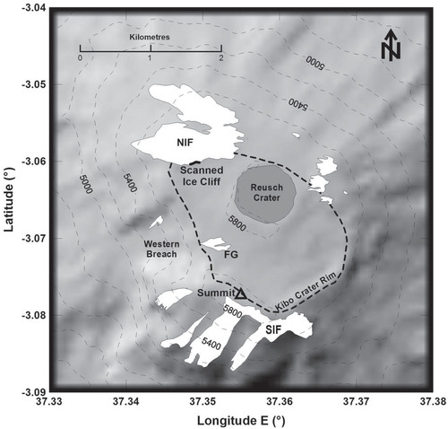
FIGURE 1. Map of Kilimanjaro showing the location of the summit ice fields and broad scan location. Contours are derived from ASTER GDEM2 data. NIF = northern ice field, SIF = southern ice field, FG = Furtwangler Glacier.

Extensive use of ablation stake measurements (Thompson et al., 2002) has been used to highlight changes in ice field thickness and extent. Mean reported rates of surface lowering during 2000–2002 approximated 1 m yr^-1 on the northern ice field (NIF) (see Fig. 1 for location). This was similar to the rates of horizontal retreat of the vertical cliffs that were reported by Thompson et al. (2002) as ∼0.92 m/yr between 2000 and 2002.These rates are perhaps surprising since one may expect that if radiative-driven recession is the dominant process, there would be much directional difference in the amount of change. Indeed the processes that control the lowering of the ice-field surface may not be synchronous with those that control the retreat of a south-facing (or north-facing) cliff.

Subsequent research by Thompson et al. (2009) implied a slower rate of thinning (or surface lowering) of 0.27 m yr^-1 on the NIF between 2000 and 2007, whereas measured lateral retreat over the same time period varied widely, but averaged 0.8 m yr^-1 along a 90 m stretch of the southern cliff of the NIF. Winkler et al. (2010) showed a slightly slower annual horizontal retreat of ∼0.75 m from March 2005 to March 2006 using a single point sonic ranging sensor. They demonstrated a seasonal contrast in retreat governed by insolation. From the beginning of March until mid-October, the rate of retreat was measured at 1.4 cm mo.^-1 (the south-facing ice wall largely shaded), increasing to 13 cm mo.^-1 during the rest of the year. They also used photogrammetric techniques to produce a three-dimensional model of a section of the ice-cliff in October 2009 (Winkler et al., 2010). This could be replicated in the future to look at distributions of loss. This paper supplements these studies by examining in more detail the spatial and temporal variability in patterns of retreat over the period 2004–2008 through detailed measurements of retreat rates on the south-facing vertical cliffs of the NIF (Fig. 1), including lowering of the surface. We use terrestrial laser-scanning technology, which we believe has not been used on Kilimanjaro previously, but is being used increasingly to measure changes in snow and ice (Grünewald et al., 2010). We examine temporal and spatial variation in retreat rates, highlighting findings obtained from detailed surveys of the south-facing ice cliff on the NIF and quantifying mean recession rates in this area. We compare our estimates with others obtained through modeling and measurement (Mölg et al., 2003b, 2008; Winkler et al., 2010). In addition, we also examine the interseasonal variation of retreat rates, which allows an examination of the forcing factors responsible.

Current Summit Environment

The current summit climate of Kilimanjaro is cold and dry. Both free air measurements (interpolated from the National Centers for Environmental Prediction [NCEP]/National Center for Atmospheric Research [NCAR] reanalysis —Kistler et al., 2001) and surface measurements of temperature and humidity on the Northern Ice Field between 2004 and 2008 (for details see Duane et al., 2008; Pepin et al., 2010) show that the mean relative humidity at crater elevation is low (<40%). This is in contrast to lower down the mountain where mean humidities and temperatures are both much higher (>70% in the case of mean relative humidity at 1800 m). Mean vapor pressure at summit elevation is around 1.6 mb, an order of magnitude lower than on the lower forested slopes. Thus, atmospheric moisture, which is required for cloud formation and precipitation, in turn essential to maintaining the summit ice fields, must be brought up the mountain from the lower slopes, since it is not present in the free-atmosphere at summit level most of the time (Troll and Wien, 1949; Mölg et al., 2009c; Pepin et al., 2010).

Much of the time the environment is characterized by lack of surface water and humidity, intense incoming radiation by day, and rapid radiative loss by night. Wind speeds are relatively low for such a high elevation (∼5800 m). Air temperatures usually remain below freezing, with mean annual temperatures between 2004 and 2008 remaining below -5 °C. Sublimation, controlled in part by the radiative balance, is the major contribution to ice field ablation (Kaser, 2001; Kaser and Osmaston, 2002; Mölg and Hardy, 2004; Winkler et al., 2009). Given this current day climate, it is surprising that summit ice fields exist at all. The exceptions to the cold dry atmosphere can occur when weak synoptic circulation can allow an upslope counterflow to transport enough moisture upslope, giving widespread cloud and precipitation over the summit crater (Mölg et al., 2009c).

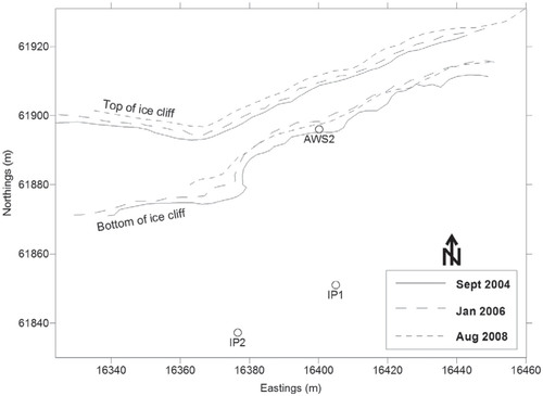
FIGURE 2. Detailed map of scanned section of the southern edge of the NIF showing survey positions IP1 and IP2. AWS2 represents the automatic weather station owned by the University of Innsbruck.

On the summit crater of Kilimanjaro, the ice-fields are sitting on slopes of very shallow gradient and thus flow dynamics are negligible (see Winkler et al., 2010). Ablation and accumulation (as controlled by climate) are thus the dominant controls of surface retreat/lowering and surface advance/raising, respectively. However, in this paper we stick to the later terms, unless discussion is in a broader climatic context.

Methodology

FIELD MEASUREMENT

The section of ice cliff chosen for survey is regular in form and coincides with sites of other instrumentation and investigations. Although the measured area is about 10%–20% of the total cliff area, it is topographically representative of the south-facing ice cliff (the most common wall orientation on the NIF) and thus the processes at work on this exposure. Its mean azimuth is around 165° (Winkler et al. [2010] reported a mean azimuth of 166° for their study). The scanned section of ice cliff is below an automatic weather station (AWS) placed by the University of Massachusetts (Amherst) on the northern ice field in 2000 and is close by another AWS (AWS 2 on Fig. 2) placed directly in front of the ice cliff by the University of Innsbruck (AWS1 and AWS2, respectively, in Winkler et al., 2010).

Automated scans of the ice cliff (Fig. 2) were taken using a servo-driven reflectorless total station (Trimble 5600 DR 200+) on three separate occasions in September 2004, January 2006, and August 2008 to determine ice cliff recession over two successive periods of 16.1 and 30.5 months. Two instrument points (IPs), spaced to cover the desired horizontal section of the ice cliff ∼140 m in length, were permanently marked in exposed basalt rock in front of the cliff (see IP1 and IP2 on Fig. 2 for locations). IP1 was assigned Universal Transverse Mercator (UTM) coordinates from a handheld global positioning system (GPS) (316405°E, 9661851°W and 5764 m elevation), and a magnetic bearing was observed to the sign at the summit of Kilimanjaro at a distance of approximately 2.2 km. The sign and its bearing was used as a reference object (RO) for the scanning total station when positioned on IP1, while bearings to three other reference objects were observed at shorter distances for use when weather conditions reduced visibility. The second instrument point IP2 (opposite the western section of the cliff) was surveyed from IP1 and the same reference objects were observed from IP2 to locate both IPs on the same coordinate system. A check measure was taken back to IP1 from IP2 with errors of 0.008 m, 0.011 m, and 0.003 m in eastings, northings, and elevation, respectively, to obtain an assessment of the accuracy of the two instrument positions. Each of the three surveys combined scans taken from both IPs to ensure the angle of incidence between the laser beam and the ice cliff was as near to normal as feasibly possible.

The total station can be used in either scanning mode, where an area is predefined by a polygon and then points measured automatically at set spatial intervals, or in manual point and record mode (an irregular sample of points is chosen). Each scan produces a large number of XYZ point measurements from which a three-dimensional surface representing the ice cliff can be interpolated. In our coordinate system (explained above and shown in Fig. 3), X is roughly perpendicular to the ice cliff, Y is parallel to the front of the cliff, and Z is elevation. The scans were taken from approximately 40 m from the base of the ice cliff with a scanning interval of 1 m in both the horizontal and vertical axes.

Additional points were surveyed using the manual point and record mode, and included in the data set. These were (a) breaklines at the top and bottom of the ice cliff, and (b) points on the ash surface. Both were subsequently used to aid in data visualization. The former were used to define cliff recession and lowering. It was easy to identify the top and bottom of the ice cliff visually and so breaklines were interpolated between points surveyed along these boundaries. The mean height along the top surveyed section was used to determine the lowering rate of the ice field surface between surveys (Table 1). Areas behind the cliff top and on the ash surface were represented by dummy points with appropriate elevations to aid visualization. The result of combining the 1 × 1 m scans with the manual and dummy points can be seen in Figure 3 showing (from the 2004 surveys) the 2530 data points on the resultant surface.

FIGURE 3. Digital elevation model (DEM) from the 2004 scan (>2000 points) showing observed data points and the slope boundaries (surveyed manually at cliff top and bottom) used in analysis of recession rates

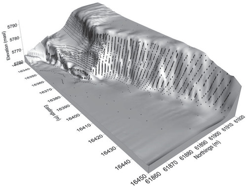
TABLE 1 Average and standard deviation of cliff-top elevations from manual observations, the difference in elevation between surveys, and the difference expressed as a rate of surface lowering per year.

Rather than simple elevational (i.e., vertical) change in Z between digital elevation models (which is partly a function of slope angle), the optimum variable to define cliff recession is slope-normal recession (see Mottershead et al., 2008, for a more detailed explanation). This acknowledges that, for similar amounts of ice-volume loss, the change in Z at a fixed point (X, Y) would be greater on steep than on shallow, or level, surfaces. To obtain slope-normal recession (SN), the mean slope angle on the ice surface (α) at each grid point is calculated from the two digital elevation models (DEMs) along with the vertical difference (V) between the two relevant grids (e.g., 2004 minus 2006).

TABLE 2 Assigned monthly weights given to account for seasonal (winter/summer) radiation budgets on the south-facing cliff. For a detailed description of how weights were assigned see the text. Figures in parentheses are adjusted to add up to 1.

Using SN to map recession rates takes slope into account. However, mapping SN over the whole domain will include areas that are not considered part of the ice cliff (i.e., the dummy points). Therefore, only the regions that were between the breaklines were selected for analysis.

Published instrument errors for the 5600DR 200+ Total Station are given by Trimble as ±3 mm ±3 ppm. Over a scanning distance of 40 m, this produces an error of <1 mm. The angular pointing error is 1″, which at a distance of 40 m again subtends an arc of less than 1 mm. Checks were carried out at the end of each survey to the ROs to confirm that the instrument had not moved. Comparing both the accuracy of the measurements (essentially ±3 mm), and the accuracy between the two IPs (<1 cm) with the measured differences between scans (averaging approximately 2 m), any errors can be seen as at least two orders of magnitude smaller than the recession rates being measured and will therefore have little impact on results.

MODELING OF SEASONAL FORCINGS

To understand climatic factors controlling recession rates in more detail, we have developed a technique to estimate the difference in recession rates between different seasons. This is possible because our scans were taken at different times of year. We have identified several climatic factors that could influence recession, including incoming radiation, cloud cover, precipitation, wind speed, and relative humidity (see the earlier discussion), but the most important in this environment is probably direct radiative input, which has a strong control on ablation. Another important influence is atmospheric moisture, which directly influences the accumulation side of the mass balance through precipitation and subsequent albedo increase, as well as indirectly through cloud cover and influence on sublimation. Assuming that each factor solely controls retreat rate, we can assign weights to each calendar month by a figure proportional to the modeled efficiency of that factor in that month (e.g., moisture, incoming radiation). We then sum up the total predicted retreat between each pair of scans (based on that factor) and using simultaneous equations we can separate seasonal contributions. Interpretation of the relative contributions of different seasons, and in particular whether realistic results are obtained, allows us to assess whether or not the modeled factor is a dominant control of recession.

Since the radiative forcing is different on the ice-field surface (we assume this is horizontal) compared with the south-facing cliff, we require different radiative models for different parts of the ice field (Cullen et al., 2007; Mölg et al., 2008). Thus, we develop separate weightings for each. Since accumulation is only possible on the ice-field surface (but is of limited relevance on the cliff, which only has an equivalent horizontal surface area of around 25% in comparison with its plan area, nearly all of it on slopes >60°), we also develop a model based on moisture but apply it only to the ice-field surface.

LATERAL RETREAT: RELATIVE CONTRIBUTIONS OF SUMMER AND WINTER RECESSION

We examine first the difference between winter and summer retreat of the ice cliff. Because Kilimanjaro is in the southern hemisphere, we use austral seasonal definitions. The south-facing ice cliff will receive more direct radiation when the sun has more of a southerly azimuth (i.e., the declination is in the southern hemisphere). Therefore each calendar month is assigned a weight based upon the amount of received solar radiation as a fraction of either winter or summer, with the weights (Table 2) being assigned based upon a cosine curve reflecting the changing solar declination across the course of the year. Within the austral summer, for example, in December the south-facing ice cliff receives more radiation (based upon incident angle) than either November or January, so December has a higher weighting. The weight thus represents how representative of “summer” conditions each month is. The winter budget is similarly constructed, but the weight represents how representative of “winter” conditions each month is, with the most positive weights being given to months with the least direct radiation input (June/July). On the south-facing ice cliff, radiative input in the two seasons (winter vs. summer) is very different, so the two halves of the year are weighted separately.

We count the relative importance of summers and winters between scans in terms of their radiation budgets, by adding up weights for months elapsed between scans. A complete summer or winter (from equinox to equinox) adds up to 1. The original weights do not appear to add up to 1 for the seasons as a whole because the astronomical seasons do not coincide with calendar months. Thus, although the weights make sense with respect to radiation input, they add up to slightly less than 1 in the table (0.988) because there is some compensation in September and March (which have some parts in both seasons). Therefore, we scale the weights so that they add up to 1 (values in brackets in Table 2). A similar process is undertaken for weighting of other factors in subsequent tables. June has a slightly lower weight than December because the austral winter is longer than the austral summer so the weighting of an individual month is slightly less, although this difference is negligible.

TABLE 3 Assigned monthly weights given to account for seasonal variations in noon solar elevation relevant to the ice-field surface. High-elevation months (noon solar elevation > 75°) are given weighting opposite to low-elevation ones. Figures in parentheses are adjusted to add up to 1.

From the scan dates, we determine how many summers and winters pass between scans and, using the recession results (Table 5, discussed later), we construct simultaneous equations to assess seasonal contributions to the recession. For the south-facing cliff where Equation 2 refers to recession during 2004–2006 and Equation 3 refers to recession during 2006–2008. The coefficients a and b on the left-hand side are derived through summing individual monthly weights over summer and winter for the respective periods, and the right-hand side (x/y) is the mean amount of retreat (in m of ice) over the respective period (calculated as an average of all points (n > 1000). We then solve for S (summer) and W (winter) recession.

SURFACE LOWERING

A similar approach can be applied to considering the lowering of the top of the ice cliff. However, using an astronomically based summer/winter weighting as in Table 2 would produce figures of limited use both because (a) the solar geometry is different on a flat surface from that on a south-facing cliff, and (b) the raising and lowering of the ice-field surface is influenced by both accumulation and ablation.

TABLE 4 Assigned monthly weights based on seasonal variations in daily mean vapor pressure at summit elevation, representative of the potential for accumulation through precipitation. Figures in parentheses are adjusted to add up to 1.

To address point a, we develop an alternative weighting based on noon solar elevation rather than solar declination (Table 3), the former being more representative of direct radiative input on a horizontal surface. In June and December, the noon solar elevation on Kilimanjaro is around 63º and 70°, respectively, but near the equinoxes the sun is overhead at noon. The weightings in Table 3 account for this, weighting months according to whether they have high or low solar elevation alone. March and September/October are weighted as having the highest solar input, and December and June/July relatively low input.

To address point b, we also develop a monthly weighting based on moisture (Table 4). The main control of surface raising is precipitation, which will be highest during the wet seasons, April–June and November–December. Unfortunately, reliable precipitation data are not available to the authors for the upper slopes of Kilimanjaro, and although scarce on the lower slopes (Hemp, 2002; Rohr and Killingtveit, 2003), it is well-known that precipitation patterns are not synchronous between the upper and lower parts of the mountain (Mölg et al., 2009c). However, we do have four years (2004–2008) of hourly vapor pressure observations taken from a Hobo datalogger sited on the NIF and use these (as a proxy for likely condensation and precipitation) to develop a wet/dry season weighting in Table 4. The use of vapor pressure instead of precipitation we believe to be fairly realistic since mean air temperatures are relatively stable throughout the year, while vapor pressure is strongly variable dependent on season (Pepin et al., 2010). The long dry period between June and September and the wet period between March and May (and also during November and December) are represented well by the weightings. Use of relative humidity to derive weightings (not shown) rather than vapor pressure makes minimal difference.

Field Results: Rates of Lateral Retreat and Surface Lowering

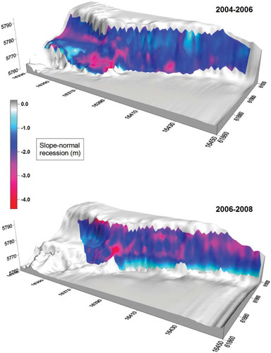
A simple visual comparison can be made by examining Figure 4, which shows slope recession for the two periods. The 2004–2006 panel shows enhanced recession at the toe of the ice cliff, whereas the opposite pattern is evident for 2006–2008. This is due to the deposition of snow or fallen ice at the foot during the 2004 and 2008 scans (austral winter) as opposed to the 2006 scan (austral summer) when this snow melts/sublimates away. Because the cliff is south-facing, it receives much more direct radiation input in the austral summer. The winter deposition at the foot results in much weaker surface change near ground level over the period 2006 to 2008. Above the foot region, most of the cliff shows recession in both periods as expected. The time elapsed between scans is longer in the second period, so absolute rates of retreat cannot be easily compared on Figure 4.

Table 5 summarizes recession rates for each period between scans with appropriate statistics and confidence intervals. Where “All” is indicated, then all data points that were selected using the digitizing method were used; however, where a range is indicated, then only the results for which the change fell within that range were used. This eliminated a few unrealistic anomalies (<5% in all cases), which were caused by two major factors: (1) points near the top of the ice cliff on the first of two scans have, over the intervening time period between scans, been lost where the ice field surface has lowered, and (2) where any of the ice cliff overhangs the vertical, the interpolation method to create the surface grid produces erroneous results. We discuss the results using the restricted range.

FIGURE 4. Three-dimensional representation of slope normal recession (m) for (upper) 2004–2006 and (lower) 2006–2008.

Although the second period, 2006–2008, shows the larger absolute recession, on a monthly basis the first period, 2004–2006, shows greater recession rates. Mean rates are 1.39 ± 0.015 m yr^-1 (period 1) and 0.89 ± 0.007 m yr^-1 (period 2). There is a significant difference in retreat rate between the two periods, but comparison of two figures alone is not long enough to infer trends. Our figures are broadly in line with past estimates based on ablation stakes and aerial photography (Thompson et al., 2002).

It is informative to compare these slope-normal retreat rates with the horizontal lowering of the surface (in Table 1), which is less than half of these rates (0.65 ± 0.38 m yr^-1 for period 1 and 0.25 ± 0.31 m yr^-1 for period 2). Error bars are larger than for wall retreat since fewer observations were taken on the surface (cliff top) and the lowering is not significantly different from zero for period 2 (at p = 0.05). Accumulation of snow on the surface possibly partially accounts for the fact that surface lowering rates are much less rapid than those of lateral cliff retreat. This horizontal lowering is again broadly in agreement with other research. Thompson et al. (2009) reports a minimum lowering of 1.9 m for the NIF between 2000 and 2007, which equates to 0.27 m yr^-1. The reduced rate in period 2 coincides with an El Niño event in East Africa that is known to encourage wetter conditions in general (Kijazi and Reason, 2009).

TABLE 5 Mean slope—normal recession rates derived from comparison of DEMs. The total (m) columns refer to the average and standard deviation of the total slope—normal recession recorded between the two scanning dates. Annual (m) figures are calculated by dividing the total recession by the number of years between the two scanning dates (16.1 months for 2004–2006 and 30.5 months for 2006–2008). The last columns refer to the number (and percentage) of points used to compute the results.

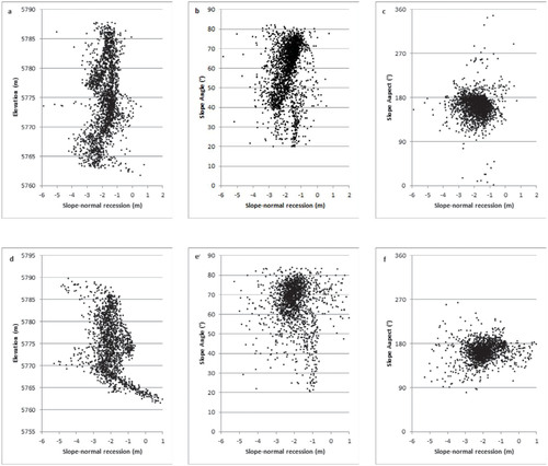
Each scan is composed of over 2500 measurements. This allows us to examine whether lateral retreat shows any relationship to specified morphological features (elevation, slope angle, and aspect) on the cliff face. Plots in Figure 5 (top row) relate to recession from 2004 to 2006 and the bottom row from 2006 to 2008. Above the foot region (which can be influenced by accumulation —e.g., Fig. 5, part d), there is no significant relationship between slope-normal recession and elevation in either period. Thus ice-cliff recession tends to be parallel. There are weak positive correlations with slope angle (more so in the first period), indicating that shallower slope angles show faster slope-normal recession, possibly a result of the incident angle to the sun's rays, particularly around solar noon. There is no significant difference in slope-normal recession between eastward- and westward-facing slope facets (although most of the cliff is within a relatively small range surrounding 165°, so the spread of aspects is small). Comparison of the two time periods shows that slope angle has the most consistent (although weak) effect on recession rate, while the other morphological features have negligible impact.

Modeling Results: Analysis of Controlling Factors

LATERAL RETREAT

Solving equations 2 and 3 produces average summer recession (S) of 1.144 ± 0.014 m and winter recession (W) of -0.11 ± 0.005 m. Errors in S and W are calculated through solving the equations for the highest and lowest possible values of x and y (based on their errors reported earlier). Although the figures hide interannual variability, the results suggest that nearly all of the recession on the southern cliff of the NIF is on average taking place during the austral summer (if we assume direct radiation as the dominant force). This realistic result corroborates other work examining the role of radiation balance in controlling ice-field recession (Mölg et al., 2003b; Winkler et al., 2010). During the winter season, direct radiation onto the wall is negligible, being restricted to early morning and very late evening. The negative value of the winter recession in the model could be explained by deposition of snow and hoar frost during this season in our scans, especially at the base of the wall.

SURFACE LOWERING

Applying the radiative (noon solar elevation) and moisture (vapor pressure) weightings and generating simultaneous equations gives different results that are not immediately intuitive. The solar weightings suggest big contrasts in surface change between high sun and low sun periods of the year. During the high sun periods, there is an average loss of 2.00 ± 0.57 m, and during the low sun periods an average gain of 1.58 ± 0.23 m. Again this suggests that local solar geometry (which is different from that on the ice cliff) is a strong driver of the surface change, since we obtain broadly realistic results.

This is not the case for the moisture model. The equations solve to a net loss of 1.58 ± 0.50 m during the wet/humid seasons, and a net gain of 1.30 ± 0.18 m during the dry seasons. The unrealistic solution implies that increased solar elevation during the humid seasons (there is some commonality between the two sets of weightings) more than compensates for the possible surface increase that should occur as a result of precipitation. Thus, even in the wetter periods of the year, there is at present not enough frequent cloud cover to prevent rapid surface lowering in the intense tropical sun (which is overhead in March and early October). Whether the concentration of lowering during the humid seasons has always been the case is unknown, but this is unlikely in the longer term.

It may appear impossible in practice for net increase in surface height to occur during the dry seasons. However, it is important to note that the figures created from solving the equations relate to the expected difference in contribution between the two different periods (wet or dry, summer or winter) and are in this sense relative, or indicative of mean interseasonal variability, assuming the weightings are realistic. They are not absolute predictions of surface change. It is therefore a useful exercise in suggesting how relative seasonal patterns in recession/lowering rates can be reconciled with controlling factors, not in deriving reliable absolute seasonal figures.

FIGURE 5. Relationships between slope normal recession (m) and morphological parameters on the southern ice cliff. Top row shows recession during 2004–2006 versus (a) elevation, (b) slope angle, and (c) aspect. Bottom row shows recession during 2006–2008 versus (d) elevation, (e) slope angle, and (f) aspect.

Discussion

The seasonal contrasts in lateral retreat are broadly in line with previous studies. Winkler et al. (2010) measured recession of the southern ice cliff of 0.168 m yr^-1 during March to mid-October, rising to 1.56 m yr^-1 during the rest of the year (sunlit period). Although slightly higher, the order of magnitude difference between austral winter and summer is similar to our results. Hastenrath (2010) reported surface lowering of 14.51 m between 1962 and 2000 (0.38 m yr^-1), which is remarkably similar to our longer-term (2004–2008) rate of 0.39 m yr^-1. The recent study of Cullen et al. (2013) concentrates on rate of surface area decrease and quotes a decline of 0.0375 km2 yr^-1 for the NIF between 2003 and 2011, with a current ice-field surface area of 0.937 km2. It is difficult to compare this directly with our measurements, but assuming a square starting area of 1 km2 (for simplicity), a loss of 0.0375 km² yr^-1would translate to a recession of ∼19 m yr^-1 on all sides of the square if the ice field was to shrink uniformly in all directions. This figure is not that sensitive to the original starting area (e.g., 1.25 km² with the same loss leads to ∼17 m yr^-1). These rates are an order of magnitude higher than all measured recession rates on the southern ice cliff, implying that recession on other exposures must be accounting for most of the measured decrease in surface area. This in turn illustrates the relative resilience of the southern ice cliff to recession.

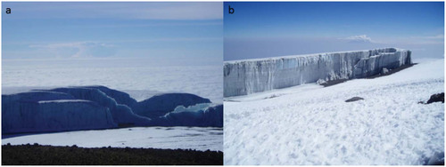
The slower rates of horizontal lowering in comparison with lateral retreat suggests that precipitation can partly compensate for the lowering driven by intense solar radiation, but there is still a long-term negative balance present. The dominance of solar geometry in explaining seasonal recession rates on the southern ice-cliff, and in overcompensating for precipitation on the surface of the ice field, agrees with much other research that shows that direct radiation is the dominant process controlling current ice-field retreat on the summit of Kilimanjaro (Kaser et al., 2004; Mölg et al., 2003b, 2009b). Further field observations made by the authors support this. Figure 6 shows two views, looking north and south from the summit to the northern and southern ice fields, respectively, during the austral winter (August) shortly after solar noon. The south face of the northern ice field is in shadow (Fig. 6, part a). Only the steeper parts of the north face of the southern ice field (Fig. 6, part b) are in shadow (but this is the season when the north face is expected to be in retreat and will receive most radiation). Both ice fields show a ridged appearance, with the development of individual elongated blocks of ice running from east to west, stacked up behind one another, thus maximizing the ice surface area exposed to either north or south, and minimizing that exposed to east or west. This orientation maximizes the protection from direct solar radiation since the accumulated radiation over the course of a year is around 50% of that on a flat surface for east/west-facing cliffs, but only 25% for north/south-facing cliffs (Fig. 7).

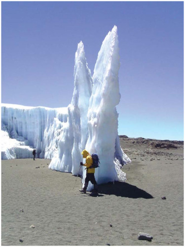
If the horizontal surface area on the top of the ice field reduces with time, surface raising through precipitation becomes less effective as a process. Thus, radiation becomes even more dominant in controlling mass balance and thus surface geometry. The increasing lateral retreat reduces the horizontal area relative to the cliff area, and herewith leads to a feedback loop whereby insolation more strongly controls the mass balance. The response is similar to the development of penitents in snow (although at a much larger spatial scale and slower temporal scale). Eventually the ice field breaks up into east-west —oriented fin-like structures (Fig. 8) with almost no horizontal surface exposed, and thus further surface accumulation becomes impossible. From this point on, the eventual demise of the ice is certain as it is no longer in equilibrium with the climatic environment.

FIGURE 6. Views looking out from the summit region of Kilimanjaro (a) looking north to the northern ice field, and (b) looking south to the southern ice field. Both photos were taken shortly after solar noon in August and demonstrate the ridged characteristics of the ice fields (approximately 30–40 m thick), maximizing opportunity for shading on the north/south-facing walls in austral summer/winter, respectively. The south face of the NIF is in shadow, whereas the north face of the SIF is largely in direct sunlight. The upper level airflow from east to west (right to left on Fig. 6, part a) can be shown by the extended anvil associated with the isolated cumulonimbus.

What is less clear is how the east-west ridges become separated from one another or from the main sheet (there is clear evidence of this process beginning on Fig. 6, part b). It is likely that local holes develop in the horizontal ice-field surface, which then become enlarged in the east/west plane through “scooping out” by the sun as it moves from east to west across the sky. What causes these holes to develop in particular locations is unknown, but once started they will easily be enlarged. This process (along with the tendency for shallow areas of ice such as the surface glaciers to disappear earlier than the thicker ice fields) means that predictions of a date for ice-field demise based purely on linear extrapolation of the rate of surface area decline into the future (e.g., Thompson et al., 2002) may be unrealistic. There may be a final period preceding disappearance when there is little or no surface area. The northern and southern ice fields are likely to split into several separate ridges before disappearing. Indeed, the Furtwangler glacier has already done so, breaking into two in 2008, and the NIF split into two in late 2012 (see report online at http://earthobservatory.nasa.gov/IOTD/view.php?id=79641), which has increased the linear distance of the ice field margin with respect to its horizontal surface area.

The concentration of horizontal lowering in the more humid periods of the year suggests that precipitation is no longer frequent or substantial enough during these seasons to counteract the increased intensity of solar radiation around the equinoxes. The continuation of strong ablation throughout the year is broadly in line with Mölg et al. (2008), who calculated seasonal ablation for a south-facing slope glacier (gradient 18° and azimuth 200°). The solar geometry was slightly different, favoring a single peak in the austral summer, rather than two peaks near the equinoxes, but interseasonal differences in ablation were slight, ranging from ∼85 mm of water equivalent per month during January–February to ∼60 mm of water equivalent per month in March–April–May (other seasons were in-between these figures). Mass balance was much more variable between seasons, but this was driven by differences in precipitation.

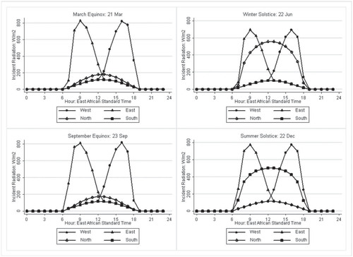
FIGURE 7. Modeled solar radiation (W/m²) received on vertical walls facing north, south, east, and west at the four main seasons (equinoxes and solstices) for Kilimanjaro. Note how north/south-facing walls receive substantial radiation only during the solstice period when the sun is in the appropriate hemisphere (one season out of four).

The modeled rapid lowering during the more humid seasons needs further validation. Since the models are based on a few years and only three scans, they may not be as robust as would be desired. El Niño events are known to influence rainfall in East Africa (Kabanda and Jury, 1999; Latif et al., 1999). There was an El Niño event during 2006–2007 (Kijazi and Reason, 2009), and this caused flooding in lowland areas of northern Tanzania, particularly during November and December, but the effects of this at the high elevations relevant to the summit ice fields are less known. Nearly all research expeditions are undertaken in the dry seasons, and the exact mechanisms of precipitation development during the wet seasons are therefore not fully understood, despite strong modeling efforts (Mölg et al., 2009c; Fairman et al., 2011; Heuser, 2010; Mölg et al., 2012).

If surface lowering is enhanced during the more humid seasons, it suggests that current cloud cover is neither frequent nor thick enough to prevent the intense (often overhead) sunlight from causing strong net lowering of the surface in-between periods of precipitation. Studies of precipitation during the wet season (Mölg et al., 2009c) have indeed suggested that heavy precipitation can occur typically only on a few days, and that even within the “wet” seasons there are many dry days with lack of cloud, particularly in the mornings. Any assumption that the wet seasons help to “top up” the ice field before it is ablated during the dry periods of the year would be erroneous.

Accumulation must have been greater than ablation during wet seasons in the past, allowing a positive mass balance to grow the ice fields. There has subsequently been a change in the character of the more humid periods of the year. Numerous studies have suggested how important atmospheric moisture is in controlling long-term mass balance on Kilimanjaro (e.g., Kaser et al., 2004; Mölg and Hardy, 2004; Mölg et al., 2006, 2009a). Substantial accumulation during successive wet seasons is required if glaciers were to start to build up again on the summit plateau (see Kaser et al., 2010, for a discussion of the recent wet season in 2006/2007 and its influence on snow buildup on the summit crater). Our results provide further evidence that the ice field was created under a different climate regime and is no longer in equilibrium with the current climate.

FIGURE 8. Photograph of final stages of ice field decline taken at Furtwangler glacier. The picture is looking east along one of the fin-like structures. The exposed surfaces face north (left) and south (right) with limited horizontal exposure and thus accumulation is now irrelevant as a mass balance component. Person gives vertical scale. Picture is taken in austral winter so sun has a northerly component (shadow on right).

Summary and Concluding Remarks

1. From three scans of the position of the south-facing cliff of the NIF on Kilimanjaro, we have quantified recession rates between 2004 and 2008. The rates of lateral retreat average 1.39 ± 0.015 m yr^-1 (2004–2006) and 0.89 ± 0.007 m yr^-1 (2006–2008). Although we acknowledge the short timescale, these rates are largely in agreement with past estimates (Thompson et al., 2002).

2. The horizontal lowering of the surface is less than half of these rates (0.65 ± 0.38 m yr^-1 for 2004–2006 and 0.25 ± 0.31 m yr^-1 for 2006–2008), again broadly consistent with Thompson's rate of 0.27 m yr^-1 for 2000–2007). Thus, on average conditions are more conducive for ice mass loss on the south-facing wall than on a flat surface, despite increased protection from direct radiation on the former.

3. An analysis of seasonal variability in recession rates confirms that on south-facing cliff of the NIF nearly all of the retreat occurs during the austral summer (September–March) when the direct radiative input is considerably higher (Cullen et al., 2007; Winkler et al., 2010). The lack of direct input in winter means recession is concentrated during half of the year.

4. On the ice-field surface itself, most of the lowering is modeled to take place in the high sun periods around the equinoxes. This again implies direct solar loading to be of critical importance in controlling lowering rather than precipitation, even on the horizontal surface. The high sun periods to some extent coincide with the more humid times (as defined by vapor pressure), leading to a somewhat unexpected concentration of surface lowering during the “humid” seasons.

Consideration of the geometry of surface recession (Figs. 6 and 8) and the spatial patterns of retreat suggests that solar geometry (Fig. 7) is the overriding factor controlling recession/lowering at this location, and is currently more influential than seasonal contributions from precipitation. We have made predictions about the future behavior of the ice-field geometry based on this information and supported by current field observations. However, our results are only representative of one location on the southern flank of the NIF. With continued and more extensive monitoring and modeling, we may be able to upscale these findings to make realistic future predictions of changes in ice-field geometry and therefore the length of survival of the ice fields, assuming a continuing similar climate regime.

Acknowledgments

We acknowledge the help of staff at TAWIRI (Tanzania Wildlife Research Institute) in granting permission for this research and, along with TANAPA (Tanzania National Parks), providing access to the Kilimanjaro National Park. We thank Tharsis Hyera, our contact at the Environmental Protection and Management Services (EPMS) for his research collaboration and help with paperwork and permits. We thank Simon Mtuy, Tim Leinbach, Francis Moshi, Emmanuel F. Mtui, and other guides and porters of Summit Expeditions and Nomadic Experience (SENE) for logistical support on the mountain. Field instrumentation was provided by the Department of Geography, University of Portsmouth. Funding was provided by the U.S. National Science Foundation, and the U.K. Royal Geographical Society Geographical Fieldwork Grant Scheme. We dedicate this paper to Emmanuel, our wonderful guide on the mountain.

References Cited

- Chan, R. Y. , Vuille, M. , Hardy, D. R. , and Bradley, R. S. , 2008: Intraseasonal precipitation variability on Kilimanjaro and the East African region and its relationship to the large-scale circulation. Theoretical and Applied Climatology , 93: 149–165, http://dx.doi.org/10.1007/s00704-007-0338-9.
- Cullen, N. J. , Mölg, T. , Kaser, G. , Hussein, K. , Steffen, K. , and Hardy, D. R. , 2006: Kilimanjaro glaciers: recent areal extent from satellite data and new interpretation of observed 20th century retreat rates. Geophysical Research Letters , 33: L16502, http://dx.doi.org/10.1029/2006GL027084.
- Cullen, N. J. , Mölg, T. , Hardy, D. R. , Steffen, K. , and Kaser, G. , 2007: Energy balance model validation on the top of Kilimanjaro using eddy correlation data. Annals of Glaciology , 46: 227–233.
- Cullen, N. J. , Sirguey, P. , Mölg, T. , Kaser, G. , Winkler, M. , and Fitzsimmons, S. J. , 2013: A century of ice retreat on Kilimanjaro: the mapping reloaded. The Cryosphere , 7: 419–431.
- Duane, W. J. , Pepin, N. C. , Losleben, M. L. , and Hardy, D. R. , 2008: General characteristics of temperature and humidity variability on Kilimanjaro, Tanzania. Arctic, Antarctic, and Alpine Research , 40: 323–334.
- Fairman, J. G. , Nair, U. S. , Christopher, S. A. , and Mölg, T. , 2011: Land use change impacts on regional climate over Kilimanjaro. Journal of Geophysical Research , 116: D03110, http://dx.doi.org/10.1029/2010JD014712.
- Grünewald, T. , Schirmer, M. , Mott, R. , and Lehning, M. , 2010: Spatial and temporal variability of snow depth and SWE in a small mountain catchment. The Cryosphere Discussions , 4: 215–225, http://dx.doi.org/10.5194/tc-4-215-2010.
- Hastenrath, S. , 2010: Climate forcing of glacier thinning on the mountains of equatorial East Africa. International Journal of Climatology , 30: 146–152.
- Hastenrath, S. , and Greischar, L. , 1997: Glacier recession on Kilimanjaro, East Africa, 1912–89. Journal of Glaciology , 43: 455–459.
- Hemp, A. , 2002: Ecology of the pteridophytes on the southern slopes of Mt. Kilimanjaro—I. Altitudinal distribution. Plant Ecology , 159(2): 211–239.
- Hemp, A. , 2005: Climate change—driven forest fires marginalize the impact of ice cap wasting on Kilimanjaro. Global Change Biology , 11: 1013–1023.
- Heuser, S. P. , 2010: The Effects of Altered Vegetation on Local Climate Change with Respect to Glaciers atop Mount Kilimanjaro. M.Sc. thesis, Department of Marine, Earth, and Atmospheric Sciences, North Carolina State University, Raleigh, 235 pp.
- Kabanda, T. A. , and Jury, M. R. , 1999: Inter-annual variability of short rains over northern Tanzania. Climate Research , 13: 231–241.
- Kaser, G. , 2001: Glacier-climate interaction at low latitudes. Journal of Glaciology , 47: 195–204.
- Kaser, G. , and Osmaston, H. , 2002: Tropical Glaciers (International Hydrology Series). Cambridge: Cambridge University Press, 207 pp.
- Kaser, G. , Hardy, D. R. , Mölg, T. , Bradley, R. S. , and Hyera, T. M. , 2004: Modern glacier retreat on Kilimanjaro as evidence of climate change: Observations and facts. International Journal of Climatology , 24(3): 329–339.
- Kaser, G. , Mölg, T. , Cullen, N. J. , Hardy, D. R. , and Winkler, M. 2010: Is the decline of ice on Kilimanjaro unprecedented in the Holocene? Holocene , 20: 1079–1091, http://dx.doi.org/10.1177/0959683610369498.
- Kijazi, A. L. , and Reason, C. J. C. , 2009: Analysis of the 2006 floods over northern Tanzania. International Journal of Climatology , 29: 955–970.
- Kistler, R. , Kalnay, E. , Collins, W. , Saha, S. , White, G. , Woollen, J. , Chelliah, M. , Ebisuzaki, W. , Kanamitsu, M. , Kousky, V. , van den Dool, H. , Jenne, R. , and Fiorino, M. , 2001: The NCEP/NCAR 50-year reanalysis. Bulletin of the American Meteorological Society , 82: 247–268.
- Lambrechts, C. , Woodley, B. , Hemp, A. , Hemp, C. , and Nyiti, P. , 2002: Aerial Survey of the Threats to Mt. Kilimanjaro Forests. New York: United Nations Development Programme, 43 pp.
- Latif, M. , Dommenget, D. , Dima, M. , and Grötzner, A. , 1999: The role of Indian Ocean SST in forcing East African rainfall anomalies during December/January 1997/98. Journal of Climate , 12: 3497–3504.
- Mölg, T. , and Hardy, D. R. , 2004: Ablation and associated energy balance of a horizontal glacier surface on Kilimanjaro. Journal of Geophysical Research , 109(D16): 1–13.
- Mölg, T. , and Kaser, G. , 2011: A new approach to resolving climate cryosphere relations: downscaling climate dynamics to glacier scale mass and energy balance without statistical scale linking. Journal of Geophysical Research , 116: D16101, http://dx.doi.org/10.1029/2011JD015669.
- Mölg, T. , Georges, C. , and Kaser, G. , 2003a: The contribution of increased incoming shortwave radiation to the retreat of the Rwenzori Glaciers, East Africa, during the 20th century. International Journal of Climatology , 23(3): 291–303.
- Mölg, T. , Hardy, D. R. , and Kaser, G. , 2003b: Solar-radiation-maintained glacier recession on Kilimanjaro drawn from combined ice-radiation geometry modelling. Journal of Geophysical Research , 108: 4731–4740, http://dx.doi.org/10.1029/2003JD003546.
- Mölg, T. , Renold, M. , Vuille, M. , Cullen, N. J. , Stocker, T. F. , and Kaser, G. , 2006: Indian Ocean zonal mode activity in a multicentury integration of a coupled AOGCM consistent with climate proxy data. Geophysical Research Letters , 33: L18710, http://dx.doi.org/10.1029/2006GL026384.
- Mölg, T. , Cullen, N. J. , Hardy, D. R. , Kaser, G. , and Klok, L. , 2008: Mass balance of a slope glacier on Kilimanjaro and its sensitivity to climate. International Journal of Climatology , 28: 881–892, http://dx.doi.org/10.1002/joc.1589.
- Mölg, T. , Cullen, N. J. , Hardy, D. R. , Winkler, M. , and Kaser, G. , 2009a: Quantifying climate change in the tropical mid-troposphere over East Africa from glacier shrinkage on Kilimanjaro. Journal of Climate , 22: 4162–4181, http://dx.doi.org/10.1175/2009JCLI2954.
- Mölg, T. , Cullen, N. J. , and Kaser, G. , 2009b: Solar radiation, cloudiness and longwave radiation over low-latitude glaciers: implications for mass balance modeling. Journal of Glaciology , 55: 292–302.
- Mölg, T. , Chiang, J. C. H. , Gohm, A. , and Cullen, N. J. , 2009c: Temporal precipitation variability versus altitude on a tropical high mountain: observations and meso-scale atmospheric modelling. Quarterly Journal of the Royal Meteorological Society , 135: 1439–1455, http://dx.doi.org/10.1002/qj.461.
- Mölg, T. , Grosshauser, M. , Hemp, A. , Hofer, M. , and Marzeion, B. , 2012: Limited forcing of glacier loss through land-use change on Kilimanjaro. Nature Climate Change , 2: 254–258, http://dx.doi.org/10.1038/NCLIMATE1390.
- Mottershead, D. N. , Duane, W. J. , Inkpen, R. J. , and Wright, J. S. , 2008: An investigation of the geometric controls on the morphological evolution of small-scale salt terrains, Cardona, Spain. Environmental Geology , 53: 1091–1098.
- Pepin, N. C. , Duane, W. , and Hardy, D. R. , 2010: The montane thermal circulation on Kilimanjaro, Tanzania and its influence on the summit ice fields: comparison of surface climate with equivalent reanalysis parameters. Global and Planetary Change , 74: 61–75.
- Rohr, P. C. , and Killingtveit, T. , 2003: Rainfall distribution on the slopes of Mt. Kilimanjaro. Journal of Hydrological Sciences , 48(1): 65–77.
- Schrumpf, M. , Axmacher, J. C. , Zech, W. , and Lyaruu, H. V. M. , 2010: Net precipitation and soil water dynamics in clearings, old secondary and old-growth forests in the montane rain forest belt of Mount Kilimanjaro, Tanzania. Hydrological Processes , 25(3): 418–428, http://dx.doi.org/10.1002/hyp.7798.
- Soini, E. , 2005: Land use change patterns and livelihood dynamics on the slopes of Mt. Kilimanjaro, Tanzania. Agricultural Systems , 85: 306–323.
- Thompson, L. G. , Mosley-Thompson, E. , Davis, M. E. , Henderson, K. A. , Brecher, H. H. , Zagorodnov, V. S. , Mashiotta, T. A. , Lin, P.-N. , Mikhalenko, V. N. , Hardy, D. R. , and Beer, J. , 2002: Kilimanjaro ice core records. Evidence of Holocene climate change in tropical Africa. Science , 298: 589–593.
- Thompson, L. G. , Brecher, H. H. , Mosley-Thompson, E. , and Hardy, D. R. , 2009: Glacier loss on Kilimanjaro continues unabated. Proceedings of the National Academy of Sciences of the United States of America , 106: 19770–19775.
- Troll, C. , and Wien, K. , 1949: Der Lewisgletscher am Mount Kenya. Geografiska Annaler , 31: 257–274.
- Winkler, M. , Juen, I. , Mölg, T. , Wagnon, P. , Gomez, J. , and Kaser, G. , 2009: Measured and modelled sublimation on the tropical Glaciar Artesonraju, Peru. Cryosphere , 3(1): 21–30.
- Winkler, M. , Kaser, G. , Cullen, N. J. , Mölg, T. , Hardy, D. R. , and Pfeffer, W. T. , 2010: Land-based marginal ice cliffs: focus on Kilimanjaro. Erdkunde , 64: 179–193, http://dx.doi.org/10.3112/erdkunde.2010.02.05,2010.