Implications of Shrinking Cryosphere Under Changing Climate on the Streamflows in the Lidder Catchment in the Upper Indus Basin, India

Abstract

Lidder tributary in the Upper Indus Basin (UIB) of the Himalayas, an important source of surface and ground water, is experiencing clear indications of climate change. In the basin, minimum, maximum, and average temperatures are showing a significant increasing trend in all the four seasons. Precipitation is showing insignificant decrease over time in the basin. However, the proportion of snow is decreasing and correspondingly, the proportion of rains is increasing. The temperature projections also show increasing trends for the end of this century. The time-series analysis of the Normalized Difference Snow Index (NDSI) shows a depletion of the snow-cover in the region. Furthermore, during the past 51 years, the glacier area in the basin has decreased from 46.09 km² in 1962 to 33.43 km² in 2013, a depletion of 27.47%. As a result of glacier recession in the basin, the streamflow fed predominantly by snowmelt and glacier melt, is showing a statistically significant decline since the mid-1990s. The declining streamflows have potential to adversely affect agriculture, energy production, tourism, and even domestic water supplies. The Snowmelt Runoff Model (SRM) was tested for estimating the runoff from this glaciated basin on an operational basis. The average simulated runoff 11.94 m³ s⁻¹ at the outlet is in concordance with the average measured runoff 13.51 m³ s⁻¹ showing R² of 0.82. The model could thus be used for snowmelt runoff estimation, on an operational basis, for judicious utilization of the depleting water resources in the region.

Introduction

Changes in the hydrological processes brought about by climate change are intimately related with the future of power generation industry health and with tourism and have far-reaching implications for the human populations, land surface processes, and ecological processes. The recent developments in mountain hydrology, coupled with the availability of new tools and observation systems, have made it possible to assess and predict the hydrological processes under changing climate at a basin scale (Green and Pickering, 2009; Munro and Marosz-Wantuch, 2009; Lutz et al., 2014). Despite the tremendous importance of mountainous water resources (Chalise et al., 2003; Chen et al., 2014) and their sensitivity to climate change (Xu et al., 2004; Arora et al., 2008; Fowler and Archer, 2006; Archer and Fowler, 2008; Shekhar et al., 2010), very few studies have been carried out in the Upper Indus Basin (UIB) to understand and characterize the impacts of climate change on the water resources in the region (Archer and Fowler, 2004; Singh and Bengtsson, 2005; Kumar et al., 2006; Tahir et al., 2011; Biemans et al., 2013; Immerzeel et al., 2013; Lutz et al., 2014; Mukhopadhyay and Khan, 2014; Romshoo and Rashid, 2014).

Predicting the long-term climate change impacts on water resources using coupled hydrological and climate models is still a very intricate task (Nurmohamed et al., 2007). Nevertheless, a number of studies have been conducted to study the impacts of climate change on hydrological processes and water resources at global scale (Christensen et al., 2004; Nurmohamed et al., 2007; Falaschi et al., 2013; Sánchez-Bayo and Green, 2013) and at regional and local scales as well (Fowler and Archer, 2005; Immerzeel et al., 2009, 2012; Mukhopadhyay and Khan, 2014). The glacier area in the Himalayas has decreased significantly in recent years as a result of increasing temperatures (Barry, 2006; UNEP, 2010). Recent research has confirmed that, for many of these glaciers, the rate of recession is accelerating (Bajracharya et al., 2008), observed mostly from the recession of the glacier snouts and mass balance studies (Kurien and Munshi, 1972; Srikanta and Pandhi, 1972; Berthier et al., 2007; Bolch et al., 2008). There are forecasts that up to a quarter of the global mountain glacier mass could disappear by 2050 and up to half could be lost by 2100 (Oerlemans, 1994; IPCC, 2007). However, there are studies that suggest that central Karakoram Range is the largest of those few areas where glaciers are showing advance (Hewitt, 2005; Bhambri et al., 2011; Tahir et al., 2011; Gardelle et al., 2012; Bahuguna et al., 2014). This dissimilarity in the glacier behavior indicates a climate change pattern in the Karakoram that differs from that in the central and eastern Himalaya (Fowler and Archer, 2006; Gardelle et al., 2012). The increase in winter precipitation since 1961 in the upper parts of the Karakoram glaciers and decrease in the summer temperature between 1961 and 2000 are regarded as the possible causes of glacier thickening in the Karakoram Range (Archer and Fowler, 2004; Fowler and Archer, 2006; Gardelle et al., 2012).

Information on the spatial and temporal variation of snow-melt runoff under changing climate is of basic interest for hydrology, water management, hydropower generation, and crop yields (Singh and Kumar, 1997; Saraf et al., 1999; Nagler and Rott, 2000; Waldner et al., 2004; Jianping et al., 2007). Understanding the spatial and temporal distribution of the snow cover and the hydro-meteorological conditions at watershed scale is also essential for the accurate prediction of snow- and glacier-melt runoff (Rango and Martinec, 1995; Singh et al., 2000; Kulkarni et al., 2002; Jain et al., 2009). In the Indus Basin, the snow- and ice-melt contribution to the stream discharge is significant in the upper portion of the basin, encompassing Kashmir and other adjacent regions of the Himalayas (Immerzeel et al., 2010). In the Kashmir Himalayas, one of the major concerns about the climate change relates to its impact on streamflows in the Indus Basin, whose waters are shared between India and Pakistan under the Indus Water Treaty. Snow and ice reserves of the Himalayan river basins, important in sustaining seasonal water availability over South Asia, are likely to be substantially affected by climate change, but to what extent is yet unclear (Immerzeel et al., 2010; Miller et al., 2012). Earlier studies have addressed the importance of glacier- and snow-melt and the potential effects of climate change downstream at various spatial scales (Barnett et al., 2005; Cyranoski, 2005; Radić et al., 2014; Bliss et al., 2014; Khan et al., 2015; Lutz et al., 2014; Rees and Collins, 2006). Therefore, a better understanding of the climate change impacts on the hydrological regime of the Himalayas is critical for the sustainable management of the water resources in the basin (Archer, 2003; Tigkas et al., 2012). In view of the tremendous economic importance of the cryosphere in the region and the fact that the glaciers in Kashmir Himalayas are receding due to climate change (Negi et al., 2009; Romshoo and Rashid, 2010), we researched to establish linkages between the depleting cryosphere, climate change, and streamflows in the Lidder catchment of the Kashmir Himalayas, India. The research emphasized and demonstrated the need for the development of a strategy for operational prediction of snow- and glacier-melt runoff from the glaciated basins of the Himalaya for optimal utilization of the depleting water resources for various sectors.

Study Region

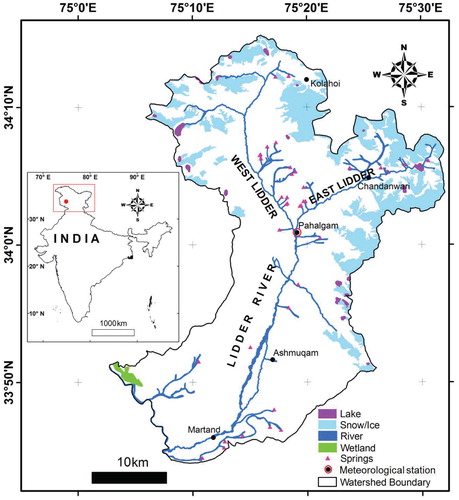
Lidder Valley is located in southeastern Kashmir in northwest Himalayas in the Upper Indus Basin, India (Fig. 1), and is spread over an area of about 1260 km².The area is precipitous mountainous terrain with an elevation ranging from 1500 to 5500 m a.s.l. and falls approximately between 75°30–E to 75°45′E longitude and 34°15′N to 34°30′N latitude. Snow covers considerable area of the catchment throughout the year, especially during the winter and spring seasons, only to melt and subsequently feed the springs and rivers during the rest of the year (Dar et al., 2013). There are about 56 glaciers in the basin, including the Kolahoi glacier, the largest glacier in the Jhelum Basin, one of the main tributaries of the Indus River. Lidder River emanating from the Kolahoi glacier is one of the main tributaries of the Jhelum Basin.

The study area exhibits a typical temperate climate with four distinct seasons viz., spring, summer, autumn, and winter. The area receives precipitation both in the form of rain and snow. On the basis of the analysis of the time series of temperature and precipitation data (1980–2010), the mean annual precipitation at the Pahalgam meteorological station is 1240 mm, with the highest rainfall recorded in the month of March (210 mm) and the lowest in the month of November (48 mm). The temperature varies between a monthly mean maximum of 19 °C in July and a minimum of -1.7 °C in January with an annual average of 9.5 °C.

Materials and Methods

In order to establish the linkages between the depleting snow and ice resources, climate change, and streamflow, we used a combination of multisource data that includes the historical precipitation and temperature data (1980–2010), historical streamflow data (1971–2011), future regional climate change model projections (2011–2098), time series of satellite images from Moderate Resolution Imaging Spectro-radiometer (MODIS) (2003, 2006–2012), SRTM Digital Elevation Data (DEM), detailed field observations, and various kinds of secondary/ancillary data. MODIS/terra snow cover Daily L3 Global 500 m Grid (MOD10A1), processed and distributed by the National Snow and Ice Data Centre (and available at http://nsidc.org),were selected to calculate the snow cover percentage on the study area (Hall and Riggs, 2007). The MODIS data of 2004–2005 are missing over the region and hence were not used in the analysis. Due to the scanty hydro-meteorological observation network in the Himalayas in general and the study area in particular, only historical data from the Pahalgam meteorological station were available for analysis in this research. A host of methods were employed to accomplish the research and included satellite images processing, geospatial techniques, statistical methods, and simulation models. Details of the data and the methods used are briefly discussed below.

ASSESSING THE INDICATORS OF CLIMATE CHANGE

The methods employed for quantifying various indicators of climate change involved the integrated use of statistical techniques, remote sensing, and Geographic Information System (GIS) as discussed here.

TREND ANALYSIS OF HYDRO-METEOROLOGICAL DATA

A time series of streamflow (1971–2011), temperature, and precipitation data (1980–2010) was used for trend analysis. The hydro-meteorological data of the basin was analyzed for trends using the Man-Kendall, Spearman's Rho, and Linear Regression statistical tests. Man-Kendall test and Spearman's Rho are nonparametric tests. The use of non-parametric tests enables us to be independent of using a number of assumptions about the population values and is well suited for analyzing trends in time series data (Gilbert, 1987). Therefore, the nonparametric Mann-Kendall statistical test was used for trend analyses of the time series of hydro-meteorological data. The test does not assume any special form for the distribution function of time series data, including missing data (Yue and Pilon, 2004). The Man-Kendall statistic is denoted by 5 and varies between -1 to +1. Rank 1 is assigned to highest value in the set. The “n” time series values (X1, X2, X3… Xn) are replaced by their relative ranks (R1, R2, R3…Rn). The test statistic S is given as:

where, sgn (x) =1 for x > 0, sgn(x) = 0 for x = 0 and sgn(x) = -1for x < 0.

If the null hypothesis H₀ is true, then S is normally distributed and its positive value is an indicator of an increasing trend.

Spearman's Rho test is widely used for determining the statistical significance of the hydro-meteorological data trends (Yue and Pilon, 2004; Bouza-Deano et al., 2008). It assesses how well an arbitrary monotonic function describes the relationship between two variables without making any other assumptions about the particular nature of the relationship between the variables. It is used when the data do not meet assumptions regarding normality, homoscedasticity, and linearity. The test static ρ_s is the correlation coefficient, which is obtained in the same way as the sample correlation coefficient but by using ranks as under:

and xi represents (time), yi (variable elements), x′ and y′ refer to ranks. In this case, x′, y′, S _x, and S _y are normally distributed with mean of zero and variance of one.

FIGURE 1. Location map of the study area. The snow cover is from IRS LISS III scene of 24 October 2005 with spatial resolution of 23.5 m. Note that elevation of Pahalgam meteorological station is 2196 m a.s.l.

Linear regression test assumes that the time series data is normally distributed by testing whether there is a linear trend by examining the relationship between time (x) and the variable of interest (y). It assumes that the errors (deviations from the trend) are independent and follows the same normal distribution with zero mean. The regression gradient is estimated by:

CLIMATE CHANGE PROJECTIONS

The future climatic data for 2011–2098 under A1B scenario was extracted for the study area from a PRECIS (Providing REgional Climates for Impact Studies) run simulated over the Kashmir valley. Average annual maximum, minimum temperature and total annual precipitation from 2011 to 2098 was analyzed for the study area, which centered at 437 ppm and 630 ppm of CO₂ concentrations for the year 2025 and 2075, respectively. Observed temperature data, procured from the Indian Meteorological Department (IMD), was upscaled to 0.5°, as the data is localized in nature, using 30-arc second GTOPO (Global TOPOgraphy) data by applying a standard atmospheric lapse rate of -0.0065 °C m^-1. This was accomplished by computing the elevation difference between a 0.5° PRECIS grid and the IMD observation station (Rashid et al., 2015). Keeping in view the capability of PRECIS in effectively simulating the climate over the Hindu-Kush Himalayan region (Akhtar et al., 2008; Dar et al., 2013; Kulkami et al., 2013; Rajbhandari et al., 2015), we chose the PRECIS model for climatological projections under the most plausible scenario, that is, A1B scenario. The use of PRECIS for climate projections under the single emission scenario could be a limitation of this research and, therefore, it would be prudent to use and validate theCMIP5 climatological projections under various scenarios with observation data from the region to check if the agreements are better. It is believed that the use of an ensemble of models and multiple scenarios would enable more possible futures in climate change over the region to be assessed.

MAPPING THE GLACIER RECESSION

Survey of India (SOI) topographic maps (1962), combined with the multi-temporal satellite images and field data, were used to map the temporal changes in glacier extent in the Lidder catchment. SOI topographic maps based on Everest Datumat at1:50,000 scale were first scanned and then geo-referenced using ground control points (GCPs). The geo-referenced topographic maps were co-registered with the satellite images. The GCPs were taken from all across the satellite image to ensure better geometric correction of the satellite data, achieving a root mean square (RMS) value <0.2 (Lillesand and Kiefer, 1987). Landsat Thematic Mapper (TM) scene of 15 October 1992, Enhanced Thematic Mapper Plus (ETM+) scene of 27 August 2000, and Landsat-8 OLI scene of 7 October 2013available from the U.S. Geological Survey (USGS) were used for the glacier mapping.The glacier boundaries and extents were extracted from the satellite image using on-screen digitization approach after applying various image enhancement, filtering, and ratio techniques to the images to highlight the glacier features so that the glacier delineation is more accurate (Racoviteanu et al., 2008; Paul and Andreassen, 2009; Paul and Svoboda, 2009; Bolch et al., 2010; Paul et al., 2013). The digital glacier outlines from the SOI topographic maps were used for comparison with the satellite-derived glacier boundaries for glacier area change assessment (1962–2013).

CHANGES IN THE SNOW COVER

A time series of MODIS data (2003, 2006–2012) was used to determine the annual snow depletion and for separating snow/ice and clouds in the Lidder catchment using Normalized Difference Snow Index (NDSI). Snow is normally mapped pixel-wise with NDSI greater than or equal to 0.4 (Hall et al., 2002; Dozier, 1989; Wang et al., 2010). However, it was observed that NDSI with 0.4 thresholds underestimates the snow cover due to the patchy snowpack in mountainous Lidder region and the effects of topography in which snow pixels are shaded by surrounding terrains (König et al., 2001). Therefore, we tried various thresholds and found the threshold of 0.36 most appropriate as it provided the best agreement between the onscreen digitized snow cover and the NDSI-derived snow cover estimates. Furthermore, we compared the NDSI-derived MODIS snow-cover map and the high resolution Landsat-ETM snow cover map to confirm that the NDSI threshold of about 0.36 is more appropriate for the snow mapping in the area.The snow cover data, along with other required variables, was used to run the SRM model for simulating discharge for the hydrological years 2007–2011.

SNOWMELT RUNOFF PREDICTION

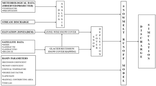
The methodology adopted for predicting snow-melt runoff from the glaciated basin is shown in Figure 2 and is based on the integrated use of remotely sensed data, digital elevation model, hydro-meteorological data, and field observations in a degree day Snowmelt-Runoff Model (SRM). SRM is designed to simulate and forecast daily streamflow in mountain basins of almost any size ranging from 0.76 to 120,000 km² with elevation ranging from 305 to 7690 m a.s.l., where snowmelt is a major runoff factor (Martinec, 1975). In degree-day approach, two temperature values each day or daily mean temperature is taken as an index variable representing all the melting factors (Blöschl, 1991; Brubaker et al., 1996; Eigdir, 2003).The overall structure of the model is described by the following equation:

where Q = average daily discharge (m³ s^-1); c = runoff coefficient for snow (index s) and rain (index r); a = degree-day factor is stated as water equivalent (cm C^-1 d^-1; T = number of degree-days (°C d) which refers to the number of positive degree days (degrees above 0 °C); ▵T = temperature lapse rate adjustment; S = ratio of the snow-covered area to the total area; P = precipitation contributing to runoff (cm); A = area of the basin or zone (km²); k = recession coefficient; n = sequence of days during the discharge computation period and 10,000/86,400 = conversion from cm km² to m³ s^-1.

Equation 10 is valid for a time lag between daily temperature cycle and the resulting discharge cycle of 18 hours (Martinec et al., 2008). T, S, and P are variables to be measured or determined each day. The degree day factor is albedo dependent. Liquid water content in the snow increases the snow density and decreases the albedo (König et al., 2001). As the melting season progresses, the snow density changes, which in turn favors the snowmelt. The degree day factor for snow can go as high as 0.6, and it usually goes higher toward the end of the summer when glacial ice becomes exposed (Rango and Martinec, 1979; Eigdir, 2003; Sharma et al., 2012). The degreeday factor values range from 0.5 to 0.6 for different months in the basin. The runoff coefficients (c _R, c _S) take into account an estimate of evapo-transpiration, sublimation of snow and ice, and percolation to deep groundwater from the basin. The c _R and c _s coefficients of the Jhelum Basin, based on calibration and validation of four years (2005–2009) discharge data, were used (Sharma et al., 2012).

FIGURE 2. Methodology adopted for accomplishing the study.

The recession coefficient (k) indicates the decline of discharge in a period without snowmelt or rainfall. Its value ranges between 0.9 to1 for various months and was derived from the equation

The normal lapse rate of -0.0065 °C ,^-1elevation increase was used. The ▵T and lag time, which are characteristics for a given basin, were taken from the literature (Sharma et al., 2012).

The precipitation data input for SRM was obtained from the Pahalgam meteorological station. The daily mean temperature data were extrapolated to the hypsometric mean elevation of different zones using the lapse rate of -0.0065 °C m^-1. A critical temperature value is specified to determine whether the measured precipitation is rain or snow and is generally above 0 °C (Charbonneau et al., 1981). Currently, a wide range of critical temperature values, based on minimum air temperature, dew point temperature, or air temperature are used to determine the form of precipitation, that is, snow or rain (Schreider et al., 1997; Marks and Winstral, 2007; Gillies et al., 2012). However, it was observed that air temperature was more reliable to determine the form of precipitation in the Lidder Basin. The critical temperature of 2 °C was employed to distinguish snowfall and rainfall events as it has been found reliable elsewhere in the Himalayan basins (Aggarwal et al., 2014). If the air temperature is higher than the critical temperature, the precipitation is rain, and if the temperature is lower than the critical temperature, the precipitation is snowfall. When the degree-day number becomes negative, it is automatically set to zero by the model so that no snowmelt is computed. Since the basin elevation ranges from 1500 to 5500 m. the Lidder Basin was subdivided into four elevation zones (Fig. 3). The average daily runoff Q was calculated by linearly summing up the runoff contributions from each elevation zone, which were calculated separately before routing (Martinec et al., 2008; Eigdir, 2003). Snow depletion curves (SDCs) were interpolated from the periodical snow cover maps to daily fractional snow cover values.

FIGURE 3. Elevation zones of the Lidder watershed.

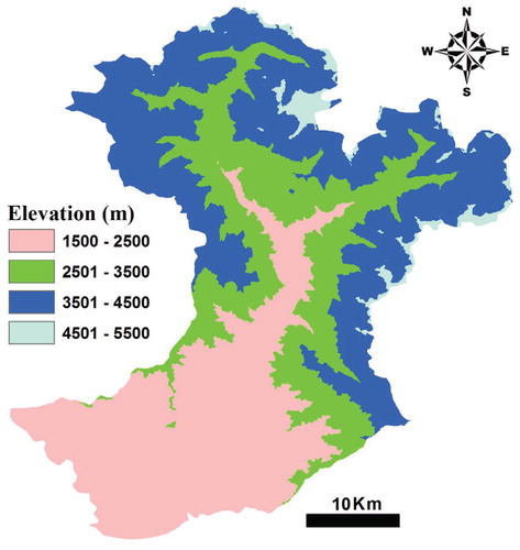
FIGURE 4. Trends in observed temperatures at Pahalgam meteorological station from 1980 to 2010. (a) Average annual temperature, (b) average minimum temperature, (c) average maximum temperature, (d) average minimum temperature in winter, (e) average maximum temperature in winter, (f) average minimum temperature in spring, (g) average maximum temperature in spring, (h) average minimum temperature in summer, (i) average maximum temperature in summer, (j) average minmum temperature in autumn, (k) average maximum temperature in autumn.

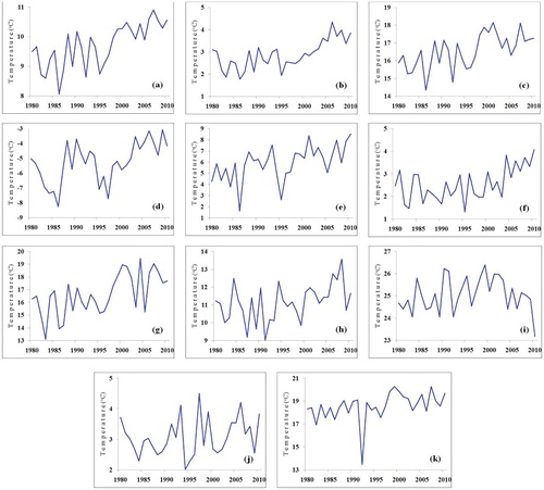
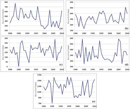
FIGURE 5. Trends in observed precipitation at Pahalgam meteorological station from 1980 to 2010. (a) Spring, (b) summer, (c) autumn, (d) winter, and (e) annual.

Results and Discussion

METEOROLOGICAL DATA TRENDS

Temperature trends for the Pahalgam meteorological station are shown in Figure 4. The mean annual temperature shows a significant increase at a < 0.01 using Man-Kendall, Spearman's Rho, and Linear Regression statistical. The maximum temperature is showing a significant increase at a < 0. The mean minimum temperature is showing significant increase at a < 0.01using both the parametric and non-parametric tests. The winter temperature is also showing increase at the significance of a < 0.01. The summer temperature is showing a significant increase at a < 0.1 for all the tests used. The spring temperature is showing a significant increase at a > 0.01. The autumn is showing a significant increase in the temperature at a < 0.05, a < 0.01, and a < 0.05 for the Man-Kendall, the Spearman's Rho, and the Linear Regression tests, respectively. The statistical significance of the annual and seasonal trends of the observed temperatures is given in Table 1.

The mean annual, winter (December–February), summer (June–August), and autumn (September–November) precipitation (Fig. 5) in the basin are showing a slightly declining but statistically insignificant trends. However, the precipitation during the spring season (March–May) shows significant decreasing trend at a < 0.05 using all the three tests. The statistical significance of the annual and seasonal trends of the observed precipitation at Pahalgam station in the basin is given in Table 2.

TABLE 1 Statistical analysis of average annual temperature, and average minimum and average maximum temperature at Pahalgam meteorological station.

CLIMATE CHANGE PROJECTIONS

Both average maximum and average minimum projected temperatures show increasing trends, whereas the projected precipitation shows a slightly decreasing trend. The mean annual maximum temperature is projected to increase by 6.26 °C (±1.84 °C) from 2011 to 2098 (Fig. 6, part a). The lowest average maximum temperature for Pahalgam meteorological station was 6.58 °C in 2011, whereas the highest maximum temperature is projected as 14.10 °C in 2096. The mean annual minimum temperature is projected to increase by 5.74 °C is (±1.50 °C) from 2011 to 2098 (Fig. 6, part b). The lowest average minimum temperature for Pahalgam was -4.82 °C in 2011, whereas the highest projected maximum temperature is -1.78 °C in 2091. The projected annual precipitation shows a very weak decreasing trend with R² of 0.048 and is not statistically significant (Fig. 6, part c). The lowest precipitation for Pahalgam is projected to be 1329.88 mm for 2067, and the highest is 2812.80 mm for 2030. Although the projected temperature is showing a good agreement with the observations, the correlation between the observed and projected precipitation is weak.

TABLE 2 Statistical analysis of annual and seasonal precipitation at Pahalgam meteorological station.

Upon comparison of the upscaled IMD data with the PRECIS projected temperatures during the baseline period, we found that the bias between the two data sets narrowed down appreciably, resulting in a good match (Fig. 7). Hence the model projections over the region are considered credible. Similar findings have been reported about the use of PRECIS in Himalayas (Kulkarni et al., 2013; Rajbhandari et al., 2015).

SNOW AND GLACIER COVER CHANGES

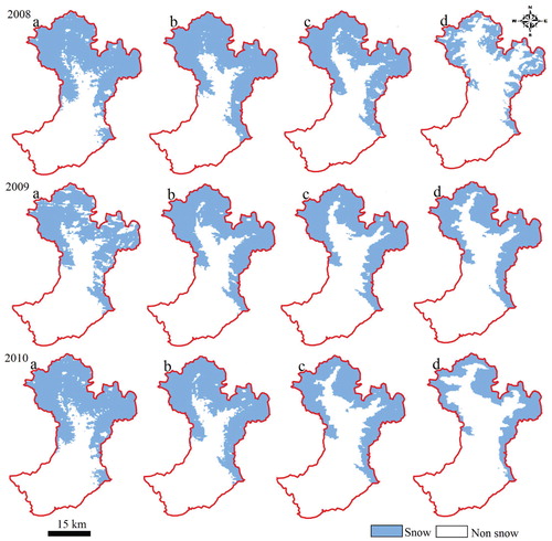
Analysis of the snow depletion curves reveals that there has been a decrease in snow precipitation since 2003–2012. Overall snow cover is very high during winter months in the study area. However, the snow begins to melt in March and the melting continues till the end of August when most of the basin is snow-free. The climate controls in the UIB are dominated by winter precipitation influenced by western disturbances (Dar et al., 2014) as opposed to the eastern and central Himalayas where monsoons are dominant (Shrestha et al., 1999; Fowler and Archer, 2005).The snow depletion curves from 2003 and 2006–2012 are shown in Figure 8, and the spatial and temporal distribution of the snow cover extent during 2006–2008 is shown in Figure 9. The spatial and temporal variations of snow-cover distribution and snowmelt runoff are considered sensitive indicators of climatic change (Wang et al., 2010). The decrease is more pronounced in winter months and could be related to the increasing minimum temperature observed during the winter months in the area. As a result of the increasing temperatures in winter, the proportion of the snow in the total precipitation is decreasing (Fig. 10). Therefore, the decreased snow precipitation is associated with the declining amount of snow on the ground. Table 3 shows the spatio-temporal changes in the Lidder Basin glacier area from 1962 to 2013. The glacier area in the basin has reduced from 46.09 km² in 1962 to 33.43 km² in 2013, showing a depletion of 27.47% in 51 years. Kolahoi, the largest glacier in the basin, has shrunk from 13.67 km² in 1962 to 10.92 km² in 2013, a decrease of 2.75 km² during the period (Fig. 11). The findings of this study support the results of the Intergovernmental Panel on Climate Change (IPCC) and the Global Land Ice Measurements from Space (GLIMS), which reported that glaciers in the Himalayas are receding faster than other parts of the world (IPCC, 2007; Immerzeel et al., 2009). The increasing temperatures and the changes in the form of precipitation (from snow to rain) are mainly responsible for the glacier recession observed in the area. The decline in the glacier- and snow-cover extent has adverse impacts on the hydrology (Sharma et al., 2012), vegetation (Rashid et al., 2015), and tourism (Dar et al., 2013) in the region. Decreased net snow accumulation on glaciers and the enhanced melting of glaciers under increasing temperatures in the region has led to glacier recession and ultimately decreased contribution to runoff from glacier melt (Archer and Fowler, 2004). Figure 12 clearly shows the impacts of the depleting cryosphere under changing climate on the streamflows in the area, the period of increasing discharge (1971–1994), and thereafter a decreasing trend (1995–2011). Keeping in view the depletion of 27.47% in the glacier area during the last 51 years, the increasing streamflow during the 1971–1994 period is attributed to the enhanced melting due to increasing temperatures, and the declining streamflows during the later period (1995–2011) is attributed to the loss of the substantial glacier mass due to the climate change witnessed in the area in the past five to six decades.

STREAMFLOW DATA TRENDS

Spatio-temporal differences in streamflow trends can occur as a result of differences in rainfall and temperature, cryosphere changes, and varying catchment characteristics that translate meteorological inputs into hydrological response (Burn and HagElnur, 2002). The trend analysis of the average yearly discharge using Man-Kendall, Spearman's Rho, and Linear Regression statistical tests at Aru hydrological station, Pahalgam, is shown in Figure 13 and Table 4. All three statistical tests show an overall significant decreasing trend for the streamflow in the basin. Analyses have also been carried out season-wise, revealing decreasing trend except for the spring season that showed a little increment in discharge.

The seasonal variation in the snow cover has significant impact on the stream discharge in the Lidder Basin as shown in Figure 13. Spring discharge shows slightly positive correlation with increasing spring temperatures. This is because the overall snow cover in the basin is at its maximum in the winter and spring seasons (February to April) and decreases substantially as the summer approaches (Fig. 8). However, temperature and discharge are negatively correlated in the summer and autumn seasons due to less snow cover on the ground and the high temperature leading to high evaporative loss and reduced runoff (Fowler and Archer, 2005). The overall discharge in the basin is showing a statistically significant decline since the mid-1990s because the overall glacial mass in the basin has decreased substantially during the past five to six decades due to the climate change (Table 3). Sharif et al. (2013) have also found a similar declining trend in runoff in the glaciated Hunza catchment at Dainyore. However, they found a significantly increasing trend in flow regime in nival catchment. Recent research has confirmed that runoff in the glaciated Karakoram constituting an important part of the Indus catchment will not decrease before the end of the 21st century (Bolch et al., 2012).

FIGURE 6. Projected temperature and precipitation for Lidder watershed (2010–2098).

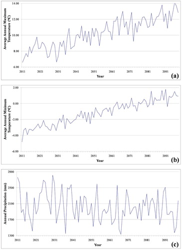
FIGURE 7. Comparison of observed temperatures from IMD and PRECIS temperature projections.

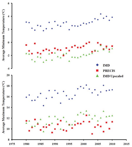
FIGURE 8. Snow depletion curves for Lidder watershed from 2003 and from 2006 to 2012.

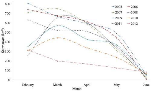
FIGURE 9. Spatio-temporal distributions of the snow cover in the study area from 2008 to 2010, in (a) February, (b) Mach, (c) April, and (d) May.

SNOWMELT RUNOFF MODELING

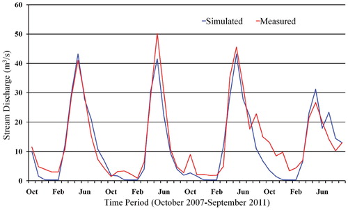
Snowmelt runoff was simulated using the SRM for the hydrological years (October–September) from 2007–2011 for the Lidder catchment in the UIB. The estimated snowmelt runoff from the basin along with the observed runoff from the catchment is shown in Figure 14.The average simulated snowmelt runoff for the catchment is 11.94 m³ s^-1, whereas the average measured runoff is13.51 m³ s^-1 The results showed a good agreement between the simulated and the measured runoff volume with r = 0.82.This demonstrates that the SRM can be used operationally to predict the streamflows of ungauged basins in the mountainous glaciated Upper Indus Basin. Typical of the glaciated Kashmir Himalayan basins, the Lidder shows a distinct summer runoff peak, compared with the more evenly distributed river flow from lowland basins that are either devoid of glaciers or receive comparatively insignificant amounts of solid precipitation. The hydrograph of the snowmelt runoff has a typical pattern reflecting the daily cycle of temperature and solar radiation. The effect of seasonal snow cover on the daily distribution of runoff in the basin is evident from the analysis of the simulated runoff. The meltwater volume is the product of the snow cover area and depth, both of which usually start decreasing by the second half of June. Generally, the computed runoff is lower than measured runoff in summer and winter periods, especially in the months October–February and May–June. This might be attributed to low snowmelt due to the reduced snow cover and less number of degree-days during the summer and winter months, respectively (Eigdir, 2003). Further, temperature and precipitation are two critical input parameters for runoff estimation and are measured at one station only and extrapolated to the entire basin assuming that they are representative for the entire basin. Depending upon the meteorological conditions, this assumption has a potential to introduce under- and over-estimation of the runoff.

Conclusion

In the glaciated basins of alpine Himalayas, with a scanty network of hydro-meteorological records, it is important to provide a reliable assessment of the snowmelt runoff so that the depleting water resources due to climate change are used more sustainably. The findings demonstrate that the changing climate in the Lidder catchment. Upper Indus, is adversely affecting the snow and glacier resources that, to date, predominantly contributed to the streamflows in the region. Depending upon the pace of climate change and the consequential shrinkage of glaciers in the region, the streamflows might plummet to critical levels, thus jeopardizing the essential uses and trans-boundary sharing of the waters in the region. It is therefore of utmost necessity to develop an operational mechanism for predicting the streamflows of the un-gauged basins in the mountainous Himalayas, so that a robust strategy is devised for the judicious and sustainable use of the depleting water resources in the region. The very good agreement between the observed and the simulated runoff shows that the SRM is a reliable simulation tool and can be used to compute daily snowmelt runoff in glaciated and snow-covered basins using only a few easily obtainable input parameters, such as hydro-meteorological data, DEM, and remote sensing-derived snow cover maps. It is hoped that the accurate assessment of the snowmelt runoff from various basins in Kashmir Himalayas in the UIB, on a routine and operational basis, shall help to develop a robust trans-boundary strategy for the conservation and optimal use of the water resources in the Indus Basin.

FIGURE 10. Trends in snow and rainfall during December–March, 1979–2011.

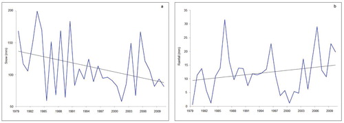
TABLE 3 Change in total glacier area of Lidder watershed and Kolahoi glacier from 1962–2013

TABLE 4 Statistical analysis of yearly and seasonal discharge at Aru, Pahalgam.

FIGURE 11. Change in spatial extent of Kolahoi glacier (1962–2013) with Landsat-8 OLI scene of 7 October 2013 in the background.

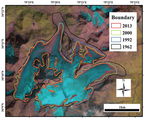
FIGURE 12. Trends in the mean annual discharge at the glacier-fed Aru gauging station, Pahalgam. Note the increasing trend in discharge from 1971 to 1994 and declining trend in discharge from 1995 to 2011.

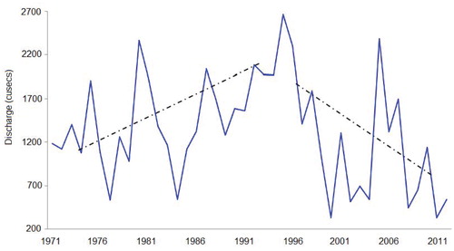
FIGURE 13. Trends in the observed discharge at Pahalgam from 1971 to 2009. (a) Discharge in spring, (b) discharge in summer, (c) discharge in autumn, (d) discharge in winter, and (e) yearly discharge.

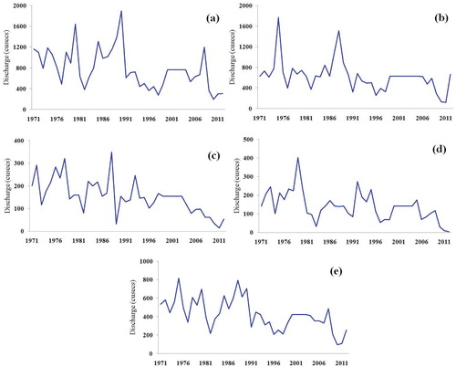
FIGURE 14. Simulated versus observed runoff using SRM model from October 2007 to September 2011.

Acknowledgments

The research work was conducted as part of the Department of Science and Technology (DST), Government of India-sponsored Inter-University Consortium research project titled “Himalayan Cryosphere: Science and Society” and the financial assistance received from the department under the project to accomplish this research is thankfully acknowledged. The authors express gratitude to the anonymous reviewers for their valuable comments and suggestions on the earlier version of the manuscript that greatly improved its content and structure.

References Cited

- Aggarwal, S. P. , Thakur, P. K. , Nikam, B. R. , and Garg, V. , 2014: Integrated approach for snowmelt run-off estimation using temperature index model, remote sensing and GIS. Current Science , 106(3): 397–407.
- Akhtar, M. , Ahmad, N. , and Booij, M. J. , 2008: The impact of climate change on the water resources of Hindukush-Karakorum-Himalaya region under different glacier coverage scenarios. Journal of Hydrology , 355(1): 148–163.
- Archer, D. R. , 2003: Contrasting hydrological regimes in Indus Basin. Journal of Hydrology , 274: 198–210.
- Archer, D. R. , and Fowler, H. J. , 2004: Spatial and temporal variations in precipitation in the Upper Indus Basin, global teleconnections and hydrological implications. Hydrology and Earth System Sciences Discussions , 8(1): 47–61.
- Archer, D. R. , and Fowler, H. J. , 2008: Using meteorological data to forecast seasonal runoff on the River Jhelum. Journal of Hydrology , 361: 10–23.
- Arora, M. , Singh, P. , Goel, N. K. , and Singh, R. D. , 2008: Climate variability influences on hydrological responses of a large Himalayan basin. Water Resources Management , 22(10): 1461–1475.
- Bahuguna, I. M. , Rathore, B. P. , Brahmbhatt, R. , Sharma, M. C. , Dhar, S. , Randhawa, S. S. , Kumar, K. , Romshoo, S. A. , Shah, R. D. , and Ganjoo, R. K. , 2014. Are the Himalayan glaciers retreating? Current Science , 106(7): 1008–1013.
- Bajracharya, S. R. , Mool, P. K. , and Shrestha, B. R. , 2008: Global climate change and melting of Himalayan glaciers. Melting Glaciers and Rising Sea Levels: Impacts and Implications. Hyderabad, India: ICFAI University Press, 28–46.
- Barnett, T. P. , Adam, J. C. , and Lettenmaier, D. P. , 2005: Potential impacts of a warming climate on water availability in snow-dominated regions. Nature , 438: 303–309.
- Barry, R. G. , 2006: The status of research on glaciers and global glacier recession: a review. Progress in Physical Geography , 30(3): 285–306.
- Berthier, E. , Arnaud, Y. , Kumar, R. , Ahmad, S. , Wagnon, P. , and Chevallier, P. , 2007: Remote sensing estimates of glacier mass balances in the Himachal Pradesh (Western Himalaya, India). Remote Sensing of Environment , 108(3): 327–338.
- Bhambri, R. , Bolch, T. , Chaujar, R. K. , and Kulshreshtha, S. C. , 2011: Glacier changes in the Garhwal Himalayas, India 1968–2006 based on remote sensing. Journal of Glaciology , 57(203): 543–556.
- Biemans, H. , Speelman, L. H. , Ludwig, F. , Moors, E. J. , Wiltshire, A. J. , Kumar, P. , Gerten, D. , and Kabat, P. , 2013: Future water resources for food production in five South Asian river basins and potential for adaptation—a modeling study. Science of the Total Environment , 468: 117–131.
- Bliss, A. , Hock, R. , and Radić, V. , 2014: Global response of glacier runoff to twenty-first century climate change. Journal of Geophysical Research: Earth Surface , 119: 1–14, doi http://dx.doi.org/10.1002/2013JF002931 .
- Blöschl, G. , 1991: The influence of uncertainty in the air temperature and albedo on snowmelt. Nordic Hydrology , 22: 95–108.
- Bolch, T. , Buchroithner, M. , Pieczonka, T. , and Kunert, A. , 2008: Planimetric and volumetric glacier changes in the Khumbu Himal, Nepal, since 1962 using Corona, Landsat TM and ASTER data. Journal of Glaciology , 54(187): 592–600.
- Bolch, T. , Yao, T. , Kang, S. , Buchroithner, M. F. , Scherer, D. , Maussion, F. , Huintjes, E. , and Schneider, C. , 2010: A glacier inventory for the western Nyainqentanglha Range and Nam Co Basin, Tibet, and glacier changes 1976–2009. The Cryosphere , 4: 419–433.
- Bolch, T. , Kulkarni, A. , Kääb, A. , Huggel, C. , Paul, F. , Cogley, J. G. , Frey, H. , Kargel, J. S. , Fujita, K. , Scheel, M. , Bajracharya, S. , and Stoffel, M. , 2012: The state and fate of Himalayan glaciers. Science , 336(6079): 310–314.
- Bouza-Deano, R. , Ternero-Rodriguez, M. , and Fernandez-Espinosa, A. J. , 2008: Trend study and assessment of surface water quality in the Ebro River (Spain). Journal of Hydrology , 361(3–4): 227–239.
- Brubaker, K. , Rango, A. , and Kustas, W. , 1996: Incorporating radiation inputs into the Snowmelt Runoff Model. Hydrological Processes , 10: 1329–1343.
- Burn, D. H. , and Hag-Elnur, M. A. , 2002: Detection of hydrologic trends and variability. Journal of Hydrology , 255: 107–122.
- Chalise, S. R. , Kansakar, S. R. , Rees, G. , Croker, K. , and Zaidman, M. , 2003: Management of water resources and low flow estimations for the Himalayan basins of Nepal. Journal of Hydrology , 282: 25–35.
- Charbonneau, R. , Lardeau, J. P. , and Obled, C. , 1981: Problems of modelling a high mountainous drainage basin with predominant snow yields. Hydrological Sciences Bulletin , 26(4): 345–361.
- Chen, R. S. , Song, Y. X. , Kang, E. S. , Han, C. T. , Liu, J. F. , Yang, Y. , Qing, W. W. , and Liu, Z. W. , 2014: A cryosphere-hydrology observation system in a small alpine watershed in the Qilian Mountains of China and its meteorological gradient. Arctic, Antarctic, and Alpine Research , 46(2): 505–523.
- Christensen, N. S. , Wood, A. W. , Voisin, N. , Lettenmaier, D. P. , and Palmer, R. N. , 2004: The effects of climate change on the hydrology and water resources of the Colorado River basin. Climatic Change , 62(1–3): 337–363.
- Cyranoski, D. , 2005: Climate change: the long-range forecast. Nature , 438: 275–276.
- Dar, R. A. , Rashid, I. , Romshoo, S. A. , and Marazi, A. , 2013: Sustainability of winter tourism in a changing climate over Kashmir Himalaya. Environmental Monitoring and Assessment , 186(4): 2549–2562.
- Dar, R. A. , Romshoo, S. A. , Chandra, R. , and Ahmad, I. , 2014: Tectono-geomorphic study of the Karewa Basin of Kashmir Valley. Journal of Asian Earth Sciences , 92: 143–156.
- Dozier, J. , 1989: Spectral signature of alpine snow cover from the Landsat Thematic Mapper. Remote Sensing of Environment , 28: 9–22.
- Eigdir, A. N. , 2003: Investigation of the snowmelt runoff in the Orumiyeh region, using modeling, GIS and remote sensing techniques. M.Sc. thesis, Enschede, Netherlands, International Institute for Geoinformation Science and Earth Observation (ITC), 66 pp.
- Falaschi, D. , Bravo, C. , Masiokas, M. , Villalba, R. , and Rivera, A. , 2013: First glacier inventory and recent changes in glacier area in the Monte San Lorenzo Region (47°S), Southern Patagonian Andes, South America. Arctic, Antarctic, and Alpine Research , 45(1): 19–28.
- Fowler, H. J. , and Archer, D. R. , 2005: Hydro-climatological variability in the Upper Indus Basin and implications for water resources. Regional Hydrological Impacts of Climatic Change—Impact Assessment and Decision Making , 295: 131–138.
- Fowler, H. J. , and Archer, D. R. , 2006: Conflicting signals of climatic change in the Upper Indus Basin. Journal of Climate , 19(17): 4276–4293.
- Gardelle, J. , Berthier, E. , and Arnaud, Y. , 2012: Slight mass gain of Karakoram glaciers in the early twenty-first century. Nature Geosciences , 5(5): 322–325.
- Gilbert, R. O. , 1987: Statistical Methods for Environmental Pollution Monitoring. New York: Van Nostrand Reinhold, 320 pp.
- Gillies, R. R. , Wang, S. Y. , and Huang, W. R. , 2012: Observational and supportive modelling analyses of winter precipitation change in China over the last half century. International Journal of Climatology , 32(5): 747–758. doi http://dx.doi.org/10.1002/Joc.2303 .
- Green, K. , and Pickering, C. M. , 2009: The decline of snowpatches in the Snowy Mountains of Australia: importance of climate warming, variable snow, and wind. Arctic, Antarctic, and Alpine Research , 41(2): 212–218.
- Hall, D. K. , and Riggs, G. A. , 2007: Accuracy assessment of the MODIS snow products. Hydrological Processes , 21(12): 1534–1547.
- Hall, D. K. , Riggs, G. A. , Solomonson, V. V. , DiGirolamo, N. E. , and Bayr, K. J. , 2002: MODIS snow cover products. Remote Sensing of Environment , 83: 181–194.
- Hewitt, K. , 2005: The Karakoram anomaly? Glacier expansion and the “elevation effect,” Karakoram Himalaya. Mountain Research and Development , 25(4): 332–340.
- Immerzeel, W. W. , Droogers, P. , De Jong, S. M. , and Bierkens, M. F. P. , 2009: Large-scale monitoring of snow cover and runoff simulation in Himalayan river basins using remote sensing. Remote Sensing of Environment , 113(1): 40–49.
- Immerzeel, W. W. , Van Beek, L. P. , and Bierkens, M. F. , 2010: Climate change will affect the Asian water towers. Science , 328: 1382–1385.
- Immerzeel, W. W. , Beek, L. P. H. , Konz, M. , Shrestha, A. B. , and Bierkens, M. F. P. , 2012: Hydrological response to climate change in a glacierized catchment in the Himalayas. Climate Change , 110: 721. doi http://dx.doi.org/10.1007/s10584-011-0143-4 .
- Immerzeel, W. W. , Pellicciotti, F. , and Bierkens, M. F. P. , 2013: Rising river flows throughout the twenty-first century in two Himalayan glacierized watersheds. Nature Geoscience , 6(9): 742–745.
- IPCC , 2007: Climate Change 2007: The Scientific Basis. Cambridge: Cambridge University Press.
- Jain, S. K. , Goswami, A. , and Saraf, A. K. , 2009: Role of elevation and aspect in snow distribution in Western Himalaya. Water Resources Management , 23(1): 71–83.
- Jianping, Y. , Yongjian, D. , Shiyin, L. , and Feng, L. J. , 2007: Variations of snow cover in the source regions of the Yangtze and Yellow Rivers in China between 1960 and 1999. Journal of Glaciology , 53(182): 420–426.
- Khan, A. , Naz, B. S. , and Bowling, L. C. , 2015: Separating snow, clean and debris covered ice in the Upper Indus Basin, Hindukush-Karakoram-Himalayas, using Landsat images between 1998 and 2002. Journal of Hydrology , 521: 46–64.
- König, M. , Winther, J. G. , and Isaksson, E. , 2001: Measuring snow and glacier ice properties from satellite. Reviews of Geophysics , 39(1): 1–27.
- Kulkarni, A. V. , Randhawa, S. S. , Rathore, B. P. , Bahuguna, I. M. , and Sood, R. K. , 2002: Snow and glacier melt runoff model to estimate hydropower potential. Journal of Indian Society Remote Sensing , 30(4): 221–228.
- Kulkarni, A. , Patwardhan, S. , Kumar, K. K. , Ashok, K. , and Krishnan, R. , 2013: Projected climate change in the Hindu Kush-Himalayan region by using the high-resolution regional climate model PRECIS. Mountain Research and Development , 33(2): 142–151.
- Kumar, K. R. , Sahai, A. K. , Krishna, K. K. , Patwardhan, K. , Mishra, P. K. , Revadekar, J. V. , Kamala, K. , and Pant, G. B. , 2006: High resolution climate change scenarios for India for the 21st century. Current Science , 90(3): 334–345.
- Kurien, M. N. , and Munshi, M. N. , 1972: A survey of Sonapani Glacier, Lahaul District, Punjab. Geological Survey of India , 15: 83–88.
- Lillesand, T. M. , and Kiefer, R. W. , 1987: Remote Sensing and Image Interpretation , Second edition. New York: John Wiley and Sons, 721 pp.
- Lutz, A. F. , Immerzeel, W. W. , Shrestha, A. B. , and Bierkens, M. F. P. , 2014: Consistent increase in High Asia's runoff due to increasing glacier melt and precipitation. Nature Climate Change , 4: 587–592.
- Marks, D. G. , and Winstral, A. H. , 2007: Finding the rain/snow transition elevation during storm events in mountain basins. Presented at Joint Symposium JHW001: Interactions Between Snow, Vegetation and the Atmosphere, 24th General Assembly of the IUGG, Perugia, Italy, 2–13 July.
- Martinec, J. , 1975: Snowmelt-runoff model for stream flow forecasts. Nordic Hydrology , 6(3): 145–154.
- Martinec, J. , Rango, A. , and Roberts, R. , 2008: Snowmelt Runoff Model (SRM) User's Manual. Edited by E. Gomez-Landesa and M. P. Bleiweiss. New Mexico State University Agricultural Experiment Station Special Report 100, 180 pp. Available at http://aces.nmsu.edu/pubs/research/weather_climate/SRMSpecRep100.pdf .
- Miller, J. D. , Immerzeel, W. W. , and Rees, G. , 2012: Climate change impacts on glacier hydrology and river discharge in the Hindu Kush-Himalayas: a synthesis of the scientific basis. Mountain Research and Development , 32(4), 461–467.
- Mukhopadhyay, B. , and Khan, A. , 2014: Rising river flows and glacial mass balance in central Karakoram. Journal of Hydrology , 513: 192–203
- Munro, D. S. , and Marosz-Wantuch, M. , 2009: Modeling ablation on Place Glacier, British Columbia, from glacier and off glacier data sets. Arctic, Antarctic, and Alpine Research , 41(2): 246–256
- Nagler, T. , and Rott, H. , 2000: Retrieval of wet snow by means of multi temporal SAR data. IEEE Transactions on Geoscience and Remote Sensing , 38(2): 754–765.
- Negi, H. S. , Thakur, N. K. , Kumar, R. , and Kumar, M. , 2009: Monitoring and evaluation of seasonal snow cover in Kashmir valley using remote sensing, GIS, and ancillary data. Journal of Earth System Sciences , 118(6): 711–720.
- Nurmohamed, R. , Naipul, S. , and De Smedt, F. , 2007: Modelling hydrological response of the upper Suriname River basin to climate change. Journal of Spatial Hydrology , 7(1): 1–22.
- Oerlemans, J. , 1994: Quantifying global warming from the retreat of glaciers. Science-AAAS-Weekly Paper Edition-including Guide to Scientific Infoimation , 264: 243–244.
- Paul, F. , and Andreassen, L. M. , 2009: A new glacier inventory for the Svartisen region, Norway, from Landsat ETM+ data: challenges and change assessment. Journal of Glaciology , 55(192): 607–618.
- Paul, F. , and Svoboda, F. , 2009: A new glacier inventory on southern Baffin Island, Canada, from ASTER data: II. Data analysis, glacier change and application. Annals of Glaciology , 50(53): 22–31.
- Paul, F. , Barrand, N. E. , Baumann, S. , Berthier, E. , Bolch, T. , Casey, K. , Frey, H. , Joshi, S. P. , Konovalov, V. , Le Bris, R. , Molg, N. , Nosenko, G. , Nuth, C. , Pope, A. , Racoviteanu, A. , Rastner, P. , Raup, B. , Scharrer, K. , Steffen, S. , and Winsvold, S. , 2013: On the accuracy of glacier outlines derived from remote-sensing data. Annals of Glaciology , 54(63): 171–182.
- Racoviteanu, A. E. , Williams, M. W. , and Barry, R. G. , 2008: Optical remote sensing of glacier characteristics: a review with focus on the Himalaya. Sensors , 8(5): 3355–3383.
- Radi, V. , Bliss, A. , Beedlow, A. C. , Hock, R. , Miles, E. , and Cogley, J. G. , 2014: Regional and global projections of twenty-first century glacier mass changes in response to climate scenarios from global climate models. Climate Dynamics , 42(1–2): 37–58.
- Rajbhandari, R. , Shrestha, A. B. , Kulkarni, A. , Patwardhan, S. K. , and Bajracharya, S. R. , 2015: Projected changes in climate over the Indus river basin using a high resolution regional climate model (PRECIS). Climate Dynamics , 44(1–2): 339–357.
- Rango, A. , and Martinec, J. , 1979: Application of a snowmelt-runoff model using Landsat data. Nordic Hydrology , 10(4): 225–238.
- Rango, A. , and Martinec, J. , 1995: Revisiting the degree day method for snowmelt computation. Journal of American Water Resources , 31(4): 657–669.
- Rashid, I. , Romshoo, S. A. , Chaturvedi, R. K. , Ravindranath, N. H. , Sukumar, R. , Jayaraman, M. , Vijaya Lakshmi, T. , and Sharma, J. , 2015: Projected climate change impacts on vegetation distribution over Kashmir Himalayas. Climatic Change : doi http://dx.doi.org/10.1007/s10584-015-1456-5 .
- Rees, H. G. , and Collins, D. N. , 2006: Regional differences in response of flow in glacier fed Himalayan rivers to climatic warming. Hydrological Processes , 20(10): 2157–2169.
- Romshoo, S. A. , and Rashid, I. , 2010: Potential and constraints of geospatial data for precise assessment of the impacts of climate change at landscape level. International Journal Geomatics and Geosciences , 1(3): 386–405.
- Romshoo, S. A. , and Rashid, I. , 2014: Assessing the impacts of changing land cover and climate on Hokersar wetland in Indian Himalayas. Arabian Journal of Geosciences , 7(1): 143–160.
- Sánchez-Bayo, F. , and Green, K. , 2013: Australian snowpack disappearing under the influence of global warming and solar activity. Arctic, Antarctic, and Alpine Research , 45(1): 107–118.
- Saraf, A. K. , Foster, J. L. , Singh, P. , and Tarafdar, S. , 1999: Passive microwave data for snow-depth and snow-extent estimations in the Himalayan Mountains. International Journal of Remote Sensing , 20(1): 83–95.
- Schreider S. Y. , Whetton, P. H. , Jakeman, A. J. , and Pittock, A. B. , 1997: Runoff modelling for snow-affected catchments in the Australian alpine region, eastern Victoria. Journal of Hydrology , 200(1–4): 1–23. doi http://dx.doi.org/10.1016/S0022-1694(97)00006-1 .
- Sharif, M. , Archer, D. R. , Fowler, H. J. , and Forsythe, N. , 2013: Trends in timing and magnitude of flow in the Upper Indus Basin. Hydrology and Earth System Sciences. 17(4): 1503–1516.
- Sharma, V. , Mishra, V. D. , and Joshi, P. K. , 2012: Snow cover variation and streamflow simulation in a snow-fed river basin of the Northwest Himalaya. Journal of Mountain Science , 9(6): 853–868.
- Shekhar, M. S. , Chand, H. , Kumar, S. , Srinivasan, K. , and Ganju, A. , 2010: Climate-change studies in the Western Himalaya. Annals of Glaciology , 51(54): 105–112.
- Shrestha, A. B. , Wake, C. , Mayewski, P. A. , and Dibb, J. , 1999: Maximum temperature trends in the Himalaya and its vicinity: an analysis based on temperature records from Nepal for the period 1971–94. Journal of Climate , 12: 2775–2786.
- Singh, P. , and Bengtsson, L. , 2005: Impact of warmer climate on melt and evaporation for the rain fed, snow fed and glaciered basins in the Himalayan region. Journal of Hydrology , 300: 140–154.
- Singh, P. , and Kumar, N. , 1997: Impact assessment of climate change on the hydrological response of a snow and glacier melt runoff dominated Himalayan River. Journal of Hydrology , 193: 316–330.
- Singh, P. , Kumar, N. , and Arora, M. , 2000: Degree day factors for snow and ice for Dokriani Glacier Garhwal Himalayas. Journal of Hydrology , 235: 1–11.
- Srikanta, S. V. , and Pandhi, R. N. , 1972: Recession of the Bada Shigri Glacier. Geological Survey of India, Miscellaneous Publications , 15: 97–100.
- Tahir, A. A. , Chevallier, P. , Arnaud, Y. , Neppel, L. , and Ahmad, B. , 2011: Modeling snowmelt-runoff under climate scenarios in the Hunza River basin, Karakoram Range, Northern Pakistan. Journal of Hydrology , 409(1): 104–117.
- Tigkas, D. , Vangelis, H. , and Tsakiris, G. , 2012: Drought and climatic change impact on streamflow in small watersheds. Science of the Total Environment , 440: 33–41.
- UNEP , 2010: The Emissions Gap Report, Are the Copenhagen Accord Pledges Sufficient to Limit Global Warming to 2 °C or 1.5 °C? Available at http://www.unep.org/publications/ebooks/emissionsgapreport .
- Waldner, P. A. , Schneebeli, M. , Schultze-Zimmermann, U. , and Flühler, H. , 2004: Effect of snow structure on water flow and solute transport. Hydrological Processes , 18: 1271–1290.
- Wang, J. , Li, H. Y. , and Hao, X. H. , 2010: Responses of snowmelt runoff to climatic change in an inland river basin, northwestern China, over the past 50a. Hydrology and Earth System Sciences Discussion , 7: 493–528.
- Xu, Z. X. , Chen, Y. N. , and Li, J. Y. , 2004: Impact of climate change on water resources in the Tarim River basin. Water Resources Management , 18(5): 439–458.
- Yue, S. , and Pilon, P. , 2004: A comparison of the power of the t-test, Mann-Kendall and bootstrap tests for trend-detection. Journal of Hydrological Sciences , 49(1): 21–37.