Using Cosmogenic ¹⁰Be Exposure Dating and Lichenometry to Constrain Holocene Glaciation in the Central Brooks Range, Alaska

ABSTRACT

We compile new and previously published lichenometric and cosmogenic ¹⁰Be moraine ages to summarize the timing of Holocene glacier expansions in the Brooks Range, Arctic Alaska. Foundational lichenometric studies suggested that glaciers likely grew to their Holocene maxima as early as the middle Holocene, followed by several episodes of moraine building prior to, and throughout, the last millennium. Previously published ¹⁰Be ages on Holocene moraine boulders from the north-central Brooks Range constrain the culmination of maximum Holocene glacier advances between 4.6 ka and 2.6 ka. New ¹⁰Be ages of moraine boulders from two different valleys in the central Brooks Range published here show that maximum Holocene glacial extents in these valleys were reached by 3.5 ka and ca. 2.6 ka, supporting previous studies showing that Holocene maximum, or near-maximum, glacial extents in the Brooks Range occurred prior to the Little Ice Age. However, in-depth reconciliations between glacier extent and local and regional climate are hampered by uncertainties associated with both lichenometry and ¹⁰Be dating.

Introduction

Declining high-latitude summer insolation through the Holocene should have driven alpine glaciers to steadily expand in the Arctic, culminating in their most extensive state during the Little Ice Age (LIA; A.D. ca. 1300–1850), prior to the recent reversal in overall Holocene cooling (Kaufman et al., 2004). In many sectors of the Arctic, the record of Holocene glaciation supports this concept, with LIA moraines most commonly being the outermost Holocene glacier deposits on the landscape. However, in the Brooks Range, well-preserved pre-LIA moraines seem to be particularly abundant. Thus, an extensive Holocene moraine record exists in the Brooks Range, providing an opportunity to develop glacier histories over a longer portion of the Holocene than is usually the case on the basis of moraine records elsewhere in the Arctic.

In light of this opportunity, we combine decades of work utilizing lichenometry (Ellis et al., 1981; Ellis and Calkin, 1981, 1984; Solomina and Calkin, 2003) and more recent cosmogenic ¹⁰Be exposure dating (hereafter ¹⁰Be dating; Badding et al., 2013) efforts in order to provide the most up-to-date compilation of data regarding Holocene glacier activity in the central Brooks Range. Our compilation expands on recent reviews of global Holocene glaciation by Solomina et al. (2015) and Holocene glaciation in Alaska by Kaufman et al. (2016), and follows scrutiny of the lichenometry method by Osborn et al. (2015). This study integrates previously published and new lichenometry and ¹⁰Be data from moraine sequences located in the central Brooks Range (Fig. 1). The comparison of data sets allows for the evaluation of the strengths and weaknesses of each dating technique as well as advancing our ability to interpret both data sets.

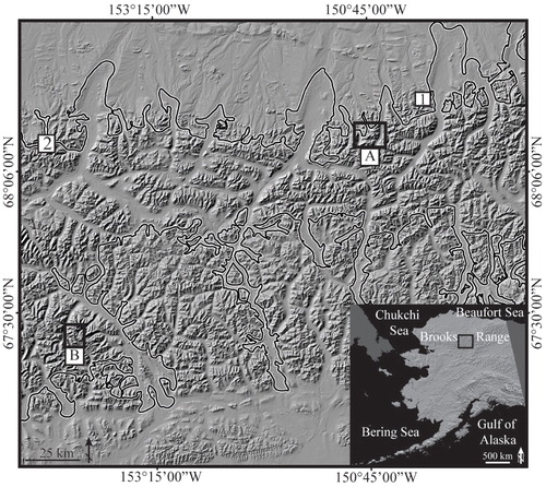
FIGURE 1. Shaded relief map of the central Brooks Range showing the (A) Erratic Creek and (B) Arrigetch Peaks study sites as well as the sites of previous work by Badding et al. (2013) at (1) Triple East Glacier and (2) Kurupa Valley. The black line denotes the Last Glacial Maximum ice limit (Kaufman et al., 2011).

Background

Stretching ∼1000 km from the Chukchi Sea in the west to the Beaufort Sea at the Alaska-Yukon border in the east, the Brooks Range forms a significant east-west physiographic and climatological barrier in Arctic Alaska (Fig. 1). The Brooks Range reaches more than 2700 m above sea level (a.s.l.) and is composed primarily of up-thrust and highly deformed Devonian sedimentary and meta-sedimentary rocks (Brosge et al., 1979). The range is heavily dissected and contains ∼1000 glaciers restricted to the highest peaks and sheltered in north-facing cirques (Ellis and Calkin, 1981; Molnia, 2007). Mean annual temperatures range from -4 to -12 °C, although recent summer temperatures at McCall Glacier, in the northeastern sector of the range, average ∼2 °C (Klok et al., 2005). The central Brooks Range receives ∼300 mm of precipitation annually (Serreze and Hurst, 2000). With most moisture coming from the southwest, precipitation rates decrease to the northeast across the range (Porter et al., 1983; Hamilton, 1986). Accordingly, the modern equilibrium-line altitudes (ELAs) of glaciers rise from ∼1766 ± 149 m a.s.l. in the west to 2027 ± 25 m a.s.l. in the east (Sikorski et al., 2009), likely because of limited moisture from the Beaufort Sea (Balascio et al., 2005).

Following the Last Glacial Maximum (LGM), glaciers in the Brooks Range retreated upvalley to, or even within, their modern limits by ca. 15 ka (Hamilton, 1986; Badding et al., 2013; Pendleton et al., 2015). Given the small extent of Brooks Range glaciers prior to the Holocene thermal maximum, during which some glaciers in southern Alaska disappeared entirely (Barclay et al., 2009), it is possible that Brooks Range glaciers may have disappeared as well. Detterman et al. (1958) and Porter and Denton (1967) first documented the existence of Holocene glacial landforms in the Brooks Range and provided a general timeline of Holocene glacier fluctuations beginning late in the Holocene. Subsequent research utilizing extensive moraine mapping and lichenometric analysis suggested that Brooks Range glaciers experienced multiple advances throughout the middle and late Holocene (Calkin and Ellis, 1980; Ellis and Calkin, 1981, 1984; Ellis et al., 1981; Haworth et al., 1986; Calkin, 1988; Sikorski et al., 2009). Despite exhaustive work carried out in the Brooks Range to reconstruct the history of Holocene glaciation, the existing lichenometric record remains largely uncorroborated by absolute dating methods, and the method has recently come under pointed scrutiny (Osborn et al., 2015).

Previously Published ¹⁰Be Ages and Lichenometry Data

Lichenometry

Lichenometric ages have been determined for Holocene moraines throughout the central Brooks Range (Appendix Table A1; Ellis et al., 1981; Ellis and Calkin, 1984; Haworth et al., 1986; Calkin, 1988; Sikorski et al., 2009). Most studies relied on the single-largest-lichen (SLL) approach, and suggested multiple pre-LIA glacier advances; some as early as ca. 4.5 ka, though most moraine activity dates to the past ca. 2 ka.

¹⁰Be Dating

In recent years, ¹⁰Be dating has been applied to Holocene moraines in the Brooks Range. Badding et al. (2013) investigated late Holocene moraines in Kurupa River valley and at the Triple East Glacier, both on the northern flank of the central Brooks Range (Fig. 1). They were the first to apply ¹⁰Be exposure dating to Holocene moraines in the Brooks Range and confirmed the presence of pre-LIA Holocene moraines indicated by lichenometry. The outermost moraines (the most extensive Holocene advance) in the Kurupa River Valley and at Triple East glacier (Fig. 1; Table 1) date to 2.7 ± 0.2 and 4.6 ± 0.5 ka, respectively. ¹⁰Be dating of moraine boulders can provide an independent chronology, providing that certain conditions are met, but the method has yet to be applied as widely as lichenometry in the Brooks Range.

Methods

Lichenometry

Lichenometric studies in the Brooks Range have largely utilized the genus Rhizocarpon because of its relative ease of identification, assumed steady growth rate, and pervasiveness across the Brooks Range. Following Calkin and Ellis (1980), all subsequent lichenometric studies applied the SLL approach (including this study), where the maximum thallus diameter of the single largest lichen measured on a moraine is used to characterize the age of each moraine using a growth curve based on radiocarbon dating of the growing surface. We interpret the “moraine age” obtained through both lichenometry and ¹⁰Be dating to reflect initial moraine stabilization following the culmination of a glacier advance. For the SLL approach, lichen measurements are taken along a traverse of the entire length of the moraine.

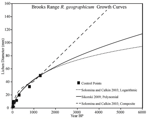
Several lichen growth curves are available for the Brooks Range (Fig. 2). The growth curve of Calkin and Ellis (1980) was updated by Solomina and Calkin (2003) and is independently constrained by radiocarbon ages for 12 lichen diameters ranging from 2 to 50 mm on surfaces dated between 20 and 1260 cal. yr B.P. (Fig. 2). Sikorski et al. (2009) produced the latest iteration of the Brooks Range growth curve by fitting a least-squares second-order polynomial to the published lichen-growth calibration data and applying a γ-intercept of 30 years to account for the colonization time of Rhizocarpon lichens (Calkin and Ellis, 1980). Sikorski et al. (2009) argued for the polynomial fit as it produces slightly younger and more realistic lichen ages (beyond 2000 cal. yr B.P.) than the logarithmic model of Solomina and Calkin (2003). In addition, it provides a better fit to the control points than the composite curve (Solomina and Calkin, 2003; Fig. 2).

We use the growth curve of Sikorski et al. (2009) to estimate ages for lichen diameters up to 150 mm. The ±20% error on lichen ages proposed by Calkin and Ellis (1980) is meant to incorporate uncertainty from moraine lithology, stability, and the effect of microclimate on lichen growth; we adopt the 20% uncertainty for all lichen ages reported herein. Because of the limited range of calibration, ages for lichens with diameters larger than ∼50 mm are considered highly uncertain because they are based on an extrapolation well beyond the control points. Furthermore, assumptions about the shape of the lichen growth curve can result in severe under- or overestimation of lichen age (Osborn et al., 2015).

¹⁰Be Dating

We used moraine morphology and lichenometric surveys in the upper Erratic Creek valley to distinguish among late Holocene moraine crests and to evaluate boulder stability for ¹⁰Be dating (Fig. 3, part a). At the Arrigetch Peak sites, we used previously published lichenometric data (Ellis et al., 1981) and new lichen surveys from this study to guide ¹⁰Be sampling (Fig. 3, part b). Moraine-crest boulders were selected based on the following characteristics: maximum height above surface, lack of apparent post-depositional movement by permafrost or mass wasting, maximum boulder size (to minimize boulder tipping or exhumation), and lichen cover and SLL diameter. The largest moraine boulders with the maximum height above the surrounding surface are the least likely to be a product of exhumation or to be affected by sediment/snow cover. Other processes, such as rock fall and glacier readvances can deposit boulders on moraines with an inherited concentration of ¹⁰Be; however, it is difficult to identify these boulders in the field, although post-sampling statistical analysis can sometimes be used to identify samples with inheritance. We collected all samples with hammer and chisel to a depth of ≤4 cm from tabular boulders with horizontal or nearly horizontal surfaces; corners and edges were avoided.

TABLE 1 New and previously published (Badding et al., 2013) ¹⁰Be moraine boulder ages and pertinent analytical data. Erratic boulders and bedrock are associated with the deglaciation of the Arrigetch valley prior to Neoglaciation (Pendleton et al., 2015).

Table

FIGURE 2. Lichen growth curves for the Brooks Range with age-control points (solid squares).

Samples were processed at the University at Buffalo Cosmogenic Isotope Laboratory following standard procedures (Kelley et al., 2012; Young et al., 2013). Following crushing and sieving to 250–850 µm, samples were pretreated in HC1 and HF-HNO₃ acid baths. Heavy-liquid mineral separation and successive heated HF-HNO₃ acid baths were used to purify quartz. ⁹Be carrier was added to quartz prior to dissolution in concentrated HF acid. Beryllium was isolated using ion-exchange chromatography and selective precipitation with NH₄OH before final oxidation to BeO.

Beryllium isotope ratios were measured at the Center for Accelerator Mass Spectrometry, Lawrence Livermore National Laboratory, and normalized against standard 07KNSTD3110 (Nishiizumi et al., 2007). Ratios of ¹⁰Be/⁹Be for process blanks averaged 1.46 ± 0.95 × 10^-15 (n = 3). ¹⁰Be ages were calculated using the CRONUS-Earth exposure-age calculator 2.3 (Balco et al., 2008) assuming no snow shielding and no erosion, and using the constant-production scaling scheme (Lm) of Lal (1991) and Stone (2000).

Because there is no ¹⁰Be production-rate-calibration site in Alaska, we must use a production-rate value from elsewhere. The most suitable production rate currently available is the Arctic production rate of Young et al. (2013), which was calibrated from sites in Arctic Canada, Greenland, and Scandinavia. The arctic production rate is indistinguishable from the ¹⁰Be production rate from northeastern North America (Balco et al., 2009), and from other recent derivations of global ¹⁰Be production rates (Heyman, 2014; Shakun et al., 2015). Finally, because the magnetic field at high latitudes is relatively constant, there is little need to temporally scale the production rate; similarly, the comparably high latitudes and moderate elevations of our sites relative to the arctic calibration sites limit the need for spatial scaling. Together, these factors increase our confidence in applying the arctic production rate in Alaska. ¹⁰Be ages are reported with 1-σG internal and external uncertainties (Table 1).

Results

Moraine Mapping and Lichenometry

Erratic Creek glacier is located at the headwaters of Erratic Creek, a tributary of the Anaktuvuk River in the north-central Brooks Range (Fig. 1). A survey of the Erratic Creek moraine revealed multiple nested crests backed by a sheer headwall (composed of tilted and deformed Devonian marine sediments, interbedded with the quartz-rich Kanayut and Middle Shainin Lake conglomerates [Moore et al., 1994]), and surrounded by steep, talus-covered slopes (Fig. 3, part a). The moraine complex has an over-steepened front with two distinct moraine crests just inboard of the front. Up-valley of these two moraine crests, the ground moraine is characterized by melt ponds, collapse features, and other obvious signs of a melting ice core. Farther up-valley is the modern ice limit, just a few tens of meters from the headwall. The moraines are boulder-dominated with little fine-grained matrix.

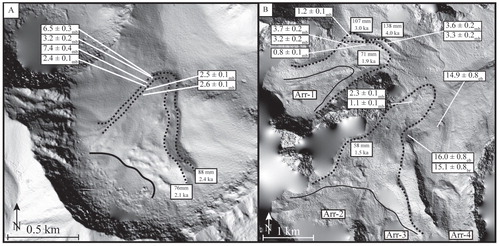
FIGURE 3. (A) Erratic Creek and (B) Arrigetch Peaks study sites with surveyed and sampled moraine crests (dashedlines), modern (2012) glacier limits (solid lines), and the single largest lichen diameter and ages. Moraine boulders (mb), erratic boulders (eh), and bedrock (br) with ¹⁰Be ages are given with 1σ uncertainties (Table 1). Note: smooth areas in shaded relief map are artifacts (imagery from University of Minnesota, Polar Geospatial Center).

At the Arrigetch Peaks location we followed Ellis et al.'s (1981) nomenclature and resurveyed and mapped the Arr-1 and Arr-2, Arr-3, and Arr-4 glaciers. In the Arr-1 cirque, we found an intact inner moraine crest with two outboard, successively older, and partially overrun moraine remnants (Fig. 3, part b). The moraine complex is ∼700 m across near the terminus, has over-steepened fronts, and contains within the complex multiple melt ponds. The moraines of Arr-1 are nestled between steep walls of granitic orthogneiss that make up the Arrigetch Peaks complex (Till et al., 2008). The Arr-2, Arr-3, and Arr-4 glaciers emanate from three cirques just south of Arr-1, but coalesce into a single tongue, which extends ∼3 km downvalley. The Arr-2, Arr-3, and Arr-4 moraine complex is composed of hummocky till deposits, multiple decomposed moraine crests, and several melt ponds all within a single over-steepened moraine crest. Both moraine suites are dominantly boulder-rich, with little matrix.

We measured lichens on moraines at both field sites and derived lichenometric ages using the growth curve of Sikorski et al. (2009). The late Holocene moraines (n = 2) of East Erratic glacier have SLL diameters of 88 and 76 mm, which yield age estimates of ca. 2.4 and 2.1 ka, respectively (Fig. 3, part a). In the Arrigetch Peaks area (Fig. 3, part b), the late Holocene moraines (n = 5) have SLL diameters of 138, 107, 71, and 58 mm, yielding ages that range from ca. 4.0, 3.0, 1.8, and 1.5 ka, respectively. We note that all measured lichens were greater than 50 mm and thus outside the lichen growth curve calibration period.

¹⁰Be Ages

In the Erratic Creek valley, moraine boulders from the outermost Holocene moraine, with a lichen diameter of 88 mm, yielded ¹⁰Be ages of 2.5 ± 0.1, 3.2 ± 0.2, 6.5 ± 0.3, and 7.4 ± 0.4 ka (Table 1; Fig. 3, part a). Boulders from the first moraine inboard of the outer most moraine with a lichen diameter of 76 mm yield ¹⁰Be ages of 2.5 ± 0.1 and 2.6 ± 0.1 ka.

In the Arrigetch Peaks area, boulders from the outer-most Holocene moraine on glacier Arr-1, with a lichen diameter of 138 mm, yielded ¹⁰Be ages of 3.3 ± 0.2 and 3.6 ± 0.2 ka (Fig. 3, part b; Table 1). A second moraine fronting glacier Arr-1, just inboard of the outermost Holocene moraine, has a lichen diameter of 107 mm and a single boulder ¹⁰Be age of 1.2 ± 0.1 ka (Fig. 3, part b). Boulders from a third moraine of Arr-1, which lies just inboard of the outer two moraines and has a lichen diameter of 71 mm, yields ¹⁰Be ages of 0.8 ± 0.1, 3.2 ± 0.2, and 3.7 ± 0.2 ka. Lastly, the outermost Holocene moraine of glaciers Arr-2, -3, and -4, which has a lichen diameter of 58 mm, yielded ¹⁰Be ages of 1.2 ± 0.1 and 2.3 ± 0.1 ka.

Discussion

Interpreting the New ¹⁰Be Chronologies

Many Brooks Range moraines, including the ones in this study, are ice-cored, which can complicate ¹⁰Be dating. Melting out of the ice core following deposition causes moraine degradation, formation of melt ponds, and the continued movement of boulders (Johnson, 1971; Lukas et al., 2005). This post-depositional boulder movement leads to ¹⁰Be ages that are younger than the true age of moraine deposition. Therefore, many ice-cored moraines have ¹⁰Be age populations ranging from the actual age of the moraine (oldest age excluding obvious older outliers due to inheritance) to progressively younger ages. ¹⁰Be ages on moraine boulders can also be older than the true timing of moraine deposition, particularly in environments with moraines in close proximity to headwalls (increasing the chance for inheritance). Though the field sites in this study are backed by steep headwalls, the moraine crests are far enough downvalley to avoid direct rockfall. Therefore, we treat the oldest, noninherited ages (as best as we can determine) as the minimum moraine age (representing the culmination of a glacial advance). These processes described above would also similarly affect lichenometric ages.

Utilizing the above criteria for boulder selection (and keeping in mind the post-depositional processes inherent to ice-cored moraines), suitable boulders were not common at either the Erratic Creek or the Arrigetch Peaks locations. Under these circumstances, the boulders sampled at each location represent the highest quality samples at each site using the selection criteria (Appendix Figs. A1–A3).

The ages from the outermost Holocene moraine of the East Erratic glacier range from 7.4 to 2.5 ka (Fig. 3, part a). The abutment of the two outermost Holocene moraines against each other with no significant intercrest trough between, and the similarity in lichen diameters (88 vs. 76 mm) suggest that the outer two moraines are similar in age and possibly represent small fluctuations of the same overall advance (Fig. 3, part a). Under this scenario, the two oldest ages on the outer moraine appear to be outliers, and the average of the four remaining ¹⁰Be ages is 2.7 ± 0.3 ka. The outliers may be boulders recycled from an older glacial deposit, or may include excess ¹⁰Be inherited from exposure in the cirque headwall. Our preferred interpretation is that the pair of nested moraines was deposited sometime between ca. 3.2 and ca. 2.5 ka, which delimits the outer-most Holocene extent of the East Erratic glacier.

The wide range of ¹⁰Be ages on the moraine crests fronting the Arrigetch Peaks glaciers Arr-1 and Arr-2 also presents challenges when interpreting moraine age. Multiple processes could lead to this wide range of boulder ages. First, as the glacier expanded into older moraine deposits, it could have incorporated previously emplaced moraine boulders into younger moraines. This recycling of boulders from older moraines into younger moraines could account for some scatter of ¹⁰Be ages from a single moraine. A second possibility involves the incorporation of talus boulders into moraines, which could account for older ¹⁰Be ages in morphostratigraphically younger moraines. Considering that the moraine is ice-cored, we prefer post-depositional modification as the most likely explanation for the presence of younger ¹⁰Be ages in older lichen zones. Interpreted this way, the maximum Holocene glacial extent in the Arrigetch Peaks likely culminated by at least ca. 3.5 ka, as evidenced by a cluster of ¹⁰Be ages around this time; additional moraine deposition occurred during subsequent millennia (Fig. 3, part b).

Uncertainty in Lichenometry

The lichenometric data provide a framework for late Holocene glacier fluctuations in the Brooks Range, albeit with complications when used as a numerical dating technique (Osborn et al., 2015). While previous workers in the Brooks Range have used the SLL to infer moraine age (e.g., Calkin and Ellis, 1980), others prefer age estimations based on larger data sets of lichen sizes (≥500) (e.g., McKinzey et al., 2004). Aside from different sampling methods, variability in growth rates from valley to valley could potentially result in large age uncertainties. Factors influencing modelled growth rates include environmental changes over time, differences between species, ongoing mortality, and inaccurate age control on calibration points (Osborn et al., 2015). Furthermore, the fitting of mathematical models to growth rates is somewhat tenuous as the general shape of growth curves is variable and poorly constrained, and different fits of the same data set can produce substantially different curves that result in significant differences in lichen age, especially beyond the calibration period.

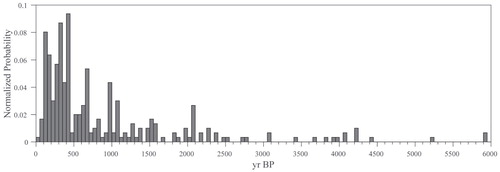
With the above caveats in mind, Figure 4 shows the cumulative lichenometric moraine data from the Brooks Range, including moraines from this study (Ellis et al., 1981; Calkin, 1988; Sikorski et al., 2009; Badding et al., 2013; Table A1). The data set indicates that glaciers were depositing moraines by at least ca. 4 ka (and likely before) followed by periods of increased moraine building at ca. 2–3, 1.5, and 1.0 ka and through the LIA (Fig. 4). The lichenometric moraine ages from this study generally agree with these periods of increased activity in the Brooks Range. However, note that the frequency distribution reflects the influence of a moraine preservation bias (older moraines overrun by younger advances) in favor of younger moraines.

Disagreement between ¹⁰Be and Lichenometry

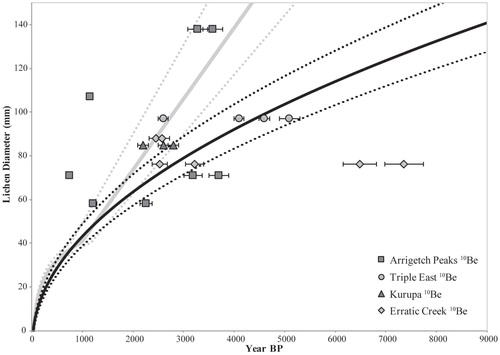
Given the sparse ¹⁰Be ages combined with the complications discussed above, and additional factors affecting lichen growth rates, moraine ages based on lichenometry and ¹⁰Be are unlikely to agree. Nevertheless, we explore the comparison of the two dating methods here. Figure 5 shows the ¹⁰Be moraine ages plotted against their corresponding lichen diameter, overlain on the two lichen growth curves widely used in the central Brooks Range (Solomina and Calkin, 2003; Sikorski et al., 2009). It is apparent that boulders from the same moraine crest (i.e., represented by the same lichen diameter) can have strikingly different ¹⁰Be ages (e.g., Erratic Creek). Conversely, moraines that yield similar ¹⁰Be ages can have inconsistent lichen diameters (e.g., Erratic Creek and Arrigetch Peaks). These conflicts within and between the two dating methods suggest that perhaps neither one is superior in this study area; both dating methods are influenced by complications common to both, and also unique to both. Figure 5 also highlights the disagreement of lichen growth curve extrapolations beyond the calibration period, and shows how the resulting age depends on which curve is chosen (e.g., Osborn et al., 2015). This disagreement between ¹⁰Be and lichen ages highlights the challenge of dating Holocene moraines in the Brooks Range using moraine boulder surface-exposure dating techniques.

FIGURE 4. Summary of moraine ages in the central Brooks Range based on lichenometry, normalized to total number of moraines sampled (using median age; n = 301; 50 yr bins). Ages were calculated using the polynomial fit of Sikorski et al. (2009) and lichen diameters reported by Calkin (1988), Sikorski et al. (2009), Badding et al. (2013), and this study.

Paleoclimatic Interpretation of Late Holocene Moraines in the Brooks Range

Under ideal circumstances, moraines are interpreted as records of climate fluctuations. However, in the Brooks Range, climate interpretations have two main limiting factors. First, as discussed above, the accuracy and precision of the lichenometric and ¹⁰Be dating techniques are limited by both shared and unique processes. Second, the size of the glaciers and the morphology of the moraines themselves could influence the exposure ages of moraine boulders in the Brooks Range. In general, Brooks Range glaciers are polythermal (Rabus and Echelmeyer, 1998; Sikorski et al., 2009), and many are relatively short and debris rich. They form voluminous moraines that small glaciers have difficulty overriding or removing from the landscape during successive advances. Thus, topographic steering of subsequent glacier advances by previously deposited, bulky moraines may result in their preservation. Therefore, the presence or absence of pre-LIA moraines may be due to characteristics intrinsic to the glaciers and not necessarily climate. Nevertheless, the abundance of pre-LIA moraines suggests that pre-LIA glaciers were at least of comparable size, if not larger, than their LIA counterparts.

FIGURE 5. Comparison of central Brooks Range Holocene moraine ages from ¹⁰Be and lichen diameters from the same moraines. The composite lichen growth curve of Solomina and Calkin (2003; gray line) and the polynomial curve of Sikorski et al. (2009; black line) are shown for comparison (dotted lines represent ±20% uncertainty on lichen ages). Also shown is the summed normalized probability density function of the ¹⁰Be ages presented in this study.

Regardless of their origin and despite the associated uncertainties, the frequency of moraines dating between ca. 2 and 5 ka provides strong evidence for pronounced pre-LIA glacial activity in the Brooks Range (Fig. 5). While the presence of pre-LIA glacial activity is common in the northern hemisphere, the apparent larger magnitude of pre-LIA advances in the Brooks Range is somewhat unusual. More commonly, glaciers in the northern hemisphere reached their maximum Holocene extent during the LIA (Karlén, 1973; Matthews, 1991; Svendsen and Mangerud, 1997) because they were driven by decreasing northern high-latitude summer insolation. For example, the most extensive Holocene glacier advance in southern Alaska occurred during the LIA (Barclay et al., 2009). Although the chronology of moraines in the Brooks Range remains uncertain, the contrasting timing of maximum Holocene glacier expansion suggests that glaciers did not respond similarly across Alaska. It is possible that drying throughout the Holocene due to arctic sea-ice cover (Funder et al., 2011) or shifting atmospheric patterns (Stone et al., 2002) restricted glacier extent during the LIA in the Brooks Range. However, the lack of tightly constrained glacier histories compounded by uncertainties related to nonclimatic processes hinders comparison with regional climate records and hampers identification of the dominant climatic controls on glacier evolution in the central Brooks Range.

Conclusions

We compiled and updated existing lichenometry data (301 moraines) and ¹⁰Be ages (21 ages from eight moraines) to summarize the chronology of middle-to-late Holocene glacier fluctuations in the central Brooks Range. The compilation of moraine lichen ages from across the Brooks Range provides a relative indicator of regional glacier history during the late Holocene. However, concerns with the method of lichen data collection, growth-rate constraints, and interpretation of ages yield large (and unquantifiable) uncertainties with lichenometry as an absolute chronometer of moraine age. The inventory of all ¹⁰Be ages of Brooks Range moraines suggests that glaciers reached their maximum Holocene extent as early as ca. 4.6 ka and experienced numerous advances throughout the late Holocene prior to the LIA. Similar to lichenometry, the ¹⁰Be method is hampered by processes intrinsic to the morphology of central Brooks Range glaciers and characteristics of their moraines. Regardless, both methods agree on the presence of relatively extensive middle and late Holocene glacier advances followed by smaller advances culminating in the LIA.

Despite decreasing northern hemisphere summer insolation throughout the Holocene, which led to most northern hemisphere glaciers reaching their Holocene maxima during the LIA, the abundance of pre-LIA moraines is conspicuous in the Brooks Range, especially compared to elsewhere in Alaska. Relative to southern Alaska, in particular, Brooks Range glaciers may have been influenced by differing climate circumstances, intrinsic morphological processes, or a combination of both. Further study and improved age constraints on Holocene glacial features are needed to better reconcile glacier chronologies and climate records.

Acknowledgments

We thank Kathryn Ladig for field assistance; Samuel Kelley, Nicolás Young, Sylvia Choi, and Mathew McClellan for laboratory assistance; Fred Luiszer for ICP measurements; and three reviewers for their helpful suggestions. This work was supported by National Science Foundation grants ARC-1107854 and ARC-1107662 to Briner and Kaufman, respectively, a Murie Science and Learning Center Fellowship and SUNY Buffalo grant to Pendleton. This is Lawrence Livermore National Laboratory contribution LLNL-JRNL-698449.

Appendix

TABLE A1 Brooks Range lichenometry.

Table

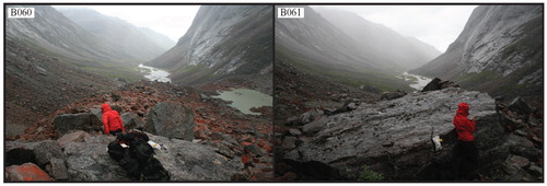
FIGURE A1. ¹⁰Be sampling.

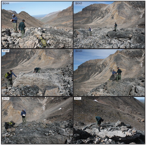
FIGURE A2. ¹⁰Be sampling (continued).

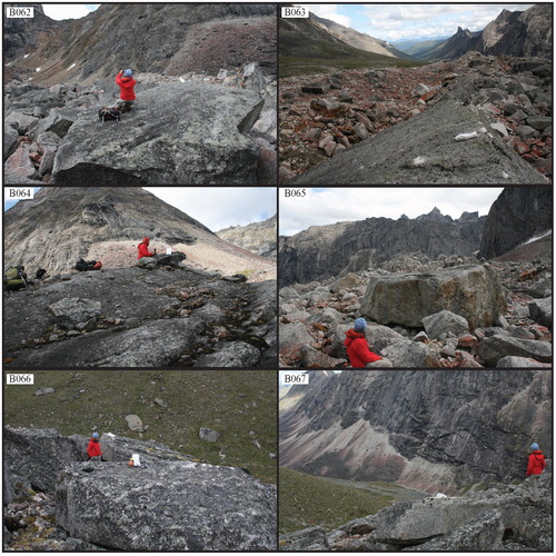
FIGURE A3. ¹⁰Be sampling (continued).

References Cited

- Badding, M. E. , Briner, J. P. , and Kaufman, D. S. , 2013: 10Be ages of late Pleistocene deglaciation and Neoglaciation in the north-central Brooks Range, Arctic Alaska. Journal of Quaternary Science , 28(1): 95–102, doi http://dx.doi.org/10.1002/jqs.2596.
- Balascio, N. L. , Kaufman, D. S. , and Manley, W. F. , 2005: Equilibrium-line altitudes during the Last Glacial Maximum across the Brooks Range, Alaska. Journal of Quaternary Science , 20(7–8): 821–838, doi http://dx.doi.org/10.1002/jqs.980 .
- Balco, G. , Stone, J. O. , Lifton, N. A. , and Dunai, T. J. , 2008: A complete and easily accessible means of calculating surface exposure ages or erosion rates from 10Be and 26Al measurements. Quaternary Geochronology , 3(3): 174–195, http://www.sciencedirect.com/science/article/pii/S1871101407000647 .
- Balco, G. , Briner, J. , Finkel, R. C. , Rayburn, J. A. , Ridge, J. C. , and Schaefer, J. M. , 2009: Regional beryllium-10 production rate calibration for late-glacial northeastern North America. Quaternary Geochronology , 4(2): 93–107, http://www.sciencedirect.com/article/pii/S1871101408000502 .
- Barclay D. J ., Wiles, G. C. , and Calkin, P. E. , 2009: Holocene glacier fluctuations in Alaska. Quaternary Science Reviews, 28(21–22): 2034–2048.
- Brosge, W. P. , Dutro, J. T. J. , and Reiser, H. N. , 1979: Bedrock Geologic Map of the Philip Smith Mountains Quadrangle, Alaska. U.S. Geological Survey Miscellaneous Field Studies Map 879-B, 2 sheets.
- Calkin, P. E. , 1988: Holocene glaciation of Alaska (and adjoining Yukon Territory, Canada). Quaternary Science Reviews , 7(2): 159–184.
- Calkin, P. E. , and Ellis, J. M. , 1980: A lichenometric dating curve and its application to Holocene glacier studies in the central Brooks Range, Alaska. Arctic and Alpine Research, 12(3): 245–264.
- Detterman, R. L. , Bowsher, A. L. , and Dutro, J. T., Jr ., 1958: Glaciation on the Arctic Slope of the Brooks Range, northern Alaska. Arctic, 11(1): 43–61.
- Ellis, J. M. , and Calkin, P. E. , 1981:A cirque-glacier chronology based on emergent lichens and mosses. Journal of Glaciology , 27(97): 511–515.
- Ellis, J. M. , and Calkin, P. E. , 1984: Chronology of Holocene glaciation, central Brooks Range, Alaska. Geological Society of America Bulletin, 95: 897–912.
- Ellis, J. M. , Hamilton, T. D. , and Calkin, P. E. , 1981: Holocene glaciation of the Arrigetch Peaks, Brooks Range, Alaska. Arctic, 34(2): 158–168.
- Funder, S. , Goosse, H. , Jepsen, H. , Kaas, E. , Kjær, K. H. , Korsgaard, N. J. , Larsen, N. K. , Linderson, H. , Lyså, A. , Möller, P. , Olsen, J. , and Willerslev, E. , 2011: A 10,000-year record of Arctic Ocean sea-ice variability—View from the beach. Science, 333(6043): 747–750, doi http://dx.doi.org/10.1126/science.1202760 .
- Hamilton, T. D. , 1986: Late Cenozoic glaciation of the central Brooks Range. In Hamilton, T. D. , Reed, K. M. , and Thorson, R. M. (eds.). Glaciation in Alaska: the Geologic Record. Anchorage: Alaska Geological Society, 9–50.
- Haworth, L. A. , Calkin, P. E. , and Ellis, J. M. , 1986: Direct measurement of lichen growth in the central Brooks Range, Alaska, U.S.A., and its application to lichenometric dating. Arctic and Alpine Research, 18(3): 289–296.
- Heyman, J. , 2014: Paleoglaciation of the Tibetan Plateau and surrounding mountains based on exposure ages and ELA depression estimates. Quaternary Science Reviews, 91: 30–41.
- Johnson, P. G. , 1971: Ice cored moraine formation and degradation, Donjek glacier, Yukon Territory, Canada. Geografiska Annaler, Series A, Physical Geography, 53(3/4): 198–202.
- Karlén, W. , 1973: Holocene glacier and climatic variations, Kebnekaise Mountains, Swedish Lapland. Geografiska Annaler. Series A, Physical Geography , 55(1): 29–63, http://www.jstor.org/stable/520485 .
- Kaufman, D. S. , Ager, T. A. , Anderson, N. J. , and 27 others, 2004: Holocene thermal maximum in the western Arctic (0–180°W). Quaternary Science Reviews , 23(5–6): 529–560, doi http://dx.doi.org/10.1016/j.quascirev.2003.09.007 .
- Kaufman, D. S. , Young, N. E. , Briner, J. P. , and Manley, W. F. , 2011: Chapter 33—Alaska palaeo-glacier atlas (version 2). In Ehlers, J. , Gibbard, P. L. , and Hughes, P. D. (eds.), Quaternary Glaciations—Extent and Chronology: a Closer Look. Amsterdam: Elsevier, 427–445, http://www.sciencedirect.com/science/article/pii/B9780444534477000337 .
- Kaufman, D. S. , Axford, Y. L. , Henderson, A. C. G. , McKay, N. P. , Oswald, W.W. , Saenger, C. , Anderson, R. S. , Bailey, H. L. , Clegg, B. , Gajewski, K. , Hu, F. S. , Jones, M. C. , Massa, C. , Routson, C. C. , Werner, A. , Wooller, M. J. , and Yu, Z. , 2016: Holocene climate changes in eastern Beringia (NW North America)—A systematic review of multiproxy evidence. Quaternary Science Reviews , 147: 311–339, http://www.sciencedirect.com/science/article/pii/S027737911530144X .
- Kelley, S.E. , Briner, J.P. , Young, N.E. , Babonis, G.S. , and Csatho, B. , 2012: Maximum late Holocene extent of the western Greenland Ice Sheet during the late 20th century. Quaternary Science Reviews 56: 89–98. http://www.sciencedirect.com/science/article/pii/S0277379112003617 .
- Klok, E. J. , Nolan, M. , and Van den Broeke, M. R. , 2005: Analysis of meteorological data and the surface energy balance of McCall Glacier,Alaska, USA. Journal of Glaciology , 51(174): 451–461.
- Lal, D. , 1991: Cosmic ray labeling of erosion surfaces: in situ nuclide production rates and erosion models. Earth and Planetary Science Letters , 104(2): 424–439.
- Lukas, S. , Nicholson, L. I. , Ross, F. H. , and Humlum, O. , 2005: Formation, meltout processes and landscape alteration of high-arctic ice-cored moraines—Examples from Nordenskiold Land, central Spitsbergen. Polar Geography , 29(3): 157–187.
- Matthews, J. A. , 1991: The late Neoglacial (‘Little Ice Age’) glacier maximum in southern Norway : new 14C-dating evidence and climatic implications. The Holocene , 1(3): 219–233, http://hol.sagepub.com/content/1/3/219.abstract .
- McKinzey, K. M. , Orwin, J. F. , and Bradwell, T. , 2004: Re-dating the moraines at Skálafellsjökull and Heinabergsjökull using different lichenometric methods: implications for the timing of the Icelandic Little Ice Age maximum. Geografiska Annaler, Series A, Physical Geography , 86(4): 319–335.
- Molnia, B. F. , 2007: Late nineteenth to early twenty-first century behavior of Alaskan glaciers as indicators of changing regional climate. Global and Planetary Change , 56(1–2): 23–56, doi http://dx.doi.org/10.1016/j.gloplacha.2006.07.011 .
- Moore, T. E. , Wallace, W. K. , Bird, K. J. , Karl, S. M. , Mull, C. G. , and Dillon, J. T. , 1994: Geology of Northern Alaska. In Plafker, G. , and Berg, H. C. (eds.), The Geology of Alaska. Boulder, Colorado: Geological Society of America, Decade of North American Geology, G-1: 49–140, http://pubs.dggsalaskagov.us/webpubs/outside/text/dnag_ch03.pdf .
- Nishiizumi, K. , Imamura, M. , Caffee, M. W. , Southon, J. R. , Finkel, R. C. , and McAninch, J. , 2007: Absolute calibration of 10Be AMS standards. Nuclear Instruments and Methods in Physics. Research Section B: Beam Interactions with Materials and Atoms , 258(2): 403–413, http://www.sciencedirect.com/science/article/pii/S0168583X07003850 .
- Osborn, G. , McCarthy, D. , LaBrie, A. , and Burke, R. , 2015: Lichenometric dating: science or pseudo-science. Quaternary Research , 83(1): 1–12.
- Pendleton, S. L. , Ceperley, E. G. , Briner, J. P. , Kaufman, D. S. , and Zimmerman, S. , 2015: Rapid and early deglaciation in the central Brooks Range, Arctic Alaska. Geology , 43(5): 419–422, http://geology.gsapubs.org/content/43/5/419.short .
- Porter, S. C. , and Denton, G. H. , 1967: Chronology of neoglaciation in the North American Cordillera. American Journal of Science 265(3): 177–210, http://www.ajsonline.org/content/265/3/177.short .
- Porter, S. C. , Pierce, K. L. , and Hamilton, T. D. , 1983: Late Wisconsin mountain glaciation in the western United States. In Porter, S. C. (ed.), The Late Pleistocene. Minneapolis: University of Minnesota Press, 71–111.
- Rabus, B. T. , and Echelmeyer, K. A. , 1998: The mass balance of McCall Glacier, Brooks Range, Alaska, USA; its regional relevance and implications for climate change in the Arctic. Journal of Glaciology , 44(147): 333–351.
- Serreze, M. C. , and Hurst, C. M. , 2000: Representation of mean arctic precipitation from NCEP-NCAR and ERA reanalyses. Journal if Climate , 13(1): 182–201.
- Shakun, J. D. , Clark, P. U. , He, F. , Lifton, N. A. , Liu, Z. , and Otto-Bliesner, B. L. , 2015: Regional and global forcing of glacier retreat during the last deglaciation. Nature Communications , 6(8059): doi http://dx.doi.org/10.1038/ncomms9059 .
- Sikorski, J. J. , Kaufman, D. S. , Manley, W. F. , and Nolan, M. , 2009: Glacial-geologic evidence for decreased precipitation during the Little Ice Age in the Brooks Range, Alaska. Arctic, Antarctic, and Alpine Research , 41(1): 138–150, doi http://dx.doi.org/10.1657/1938-4246(07-078)[SIKORSKI]2.0.CO;2.
- Solomina, O. , and Calkin, P. E. , 2003: Lichenometry as applied to moraines in Alaska, U.S.A., and Kamchatka, Russia. Arctic, Antarctic, and Alpine Research , 35(2): 129–143.
- Solomina, O. N. , Bradley, R. S. , Hodgson, D. A. , Ivy-Ochs, S. , Jomelli, V. , Mackintosh, A. N. , Nesje, A. , Owen, L. A. , Wanner, H. , Wiles, G. C. , and Young, N. E. , 2015: Holocene glacier fluctuations. Quaternary Science Reviews 111: 9–34, http://www.sciencedirect.com/science/article/pii/S0277379114004788 .
- Stone, J. O. , 2000: Air pressure and cosmogenic isotope production. Journal of Geophysical Research Solid Earth , 105(B10): 23753–23759.
- Stone, R. S. , Dutton, E. G. , Harris, J. M. , and Longenecker, D. , 2002: Earlier spring snowmelt in northern Alaska as an indicator of climate change. Journal of Geophysical Research: Atmospheres , 107(D10): ACL 10-1-ACL 10–13.
- Svendsen, J. I. , and Mangerud, J. , 1997: Holocene glacial and climatic variations on Spitsbergen, Svalbard. The Holocene 7(1): 45–57, http://hol.sagepub.com/content/7/1/45.abstract .
- Till, A. B. , Dumoulin, J. A. , Harris, A. G. , Moore, T. E. , Bleick, H. A. , Siwiec, B. R. , 2008: Bedrock Geologic Map of the Southern Brooks Range, Alaska, and Accompanying Conodont Data. U.S. Geological Survey Open-File Report 2008–1149: 88 pp., http://citeseerx.ist.psu.edu/viewdoc/download?doi=10.1.1.405.7955&rep=rep1&type=pdf .
- Young, N. E. , Schaefer, J. M. , Briner, J. P. , and Goehring, B. M. , 2013: A 10Be production-rate calibration for the Arctic. Journal of Quaternary Science , 28(5): 515–526, http://onlinelibrary.wiley.com/doi/10.1002/jqs.2642/full .