Techniques for estimating health care costs with censored data: an overview for the health services researcher

Abstract

Objective

The aim of this study was to review statistical techniques for estimating the mean population cost using health care cost data that, because of the inability to achieve complete follow-up until death, are right censored. The target audience is health service researchers without an advanced statistical background.

Methods

Data were sourced from longitudinal heart failure costs from Ontario, Canada, and administrative databases were used for estimating costs. The dataset consisted of 43,888 patients, with follow-up periods ranging from 1 to 1538 days (mean 576 days). The study was designed so that mean health care costs over 1080 days of follow-up were calculated using naïve estimators such as full-sample and uncensored case estimators. Reweighted estimators – specifically, the inverse probability weighted estimator – were calculated, as was phase-based costing. Costs were adjusted to 2008 Canadian dollars using the Bank of Canada consumer price index (http://www.bankofcanada.ca/en/cpi.html).

Results

Over the restricted follow-up of 1080 days, 32% of patients were censored. The full-sample estimator was found to underestimate mean cost ($30,420) compared with the reweighted estimators ($36,490). The phase-based costing estimate of $37,237 was similar to that of the simple reweighted estimator.

Conclusion

The authors recommend against the use of full-sample or uncensored case estimators when censored data are present. In the presence of heavy censoring, phase-based costing is an attractive alternative approach.

Keywords:

• health care costing
• heart failure
• incomplete data
• statistical techniques
• phase-based costing

Introduction

Accurate estimates of health care costs have a wide range of applications and are of growing importance to both policy makers and clinicians, given the burgeoning costs of health care delivery, budgetary constraints, and the aging population. Therefore, it is important for health services researchers to be familiar with robust methods for description, inference, and prediction using costing data.

A number of statistical properties of costing data preclude the use of traditional statistical tools.^1,2 There is a rich econometric and statistical literature focused predominantly on three specific properties of cost data: first, a substantial proportion of the general population may be healthy, requiring little medical care and having zero costs; second, the distribution of health care costs for those who do incur costs is usually heavily right skewed, with a few very high-cost individuals on the tail; third, investigators have shown that the assumption of homoscedasticity (ie, constant variance in the error term) is often violated and thereby alternative modeling techniques are required.^2–6

A fourth obstacle is incomplete data when health care expenses are not available for all participants for the entire period of interest. Although this area is one of active research, much of this work has been presented in health economics or statistical journals.^3,7–13 The objective of the present review is to examine this fourth obstacle in detail, targeting an audience of health services researchers without an advanced statistical background. The authors will focus on the basic operation of estimating mean health care costs, using both simulations and a case study to illustrate these concepts. In the process, the goal is to provide some of the necessary background to make this important area of study more accessible.

The case study was of patients with heart failure (HF) in Ontario, Canada.¹⁴ Briefly, all patients with an admission for HF, based on International Classification of Disease Version 10 Code I50, during the period 2004–2006 were identified in the Canadian Institute for Health Information’s Discharge Abstract Database. Costs for hospital admission, same-day surgeries, physician services, ambulatory care, and HF medications were estimated in 30-day intervals until March 31, 2008.¹⁴ Throughout the text, the example of cumulative 3-year costs, approximated as 1080 days based on the 30-day costing interval, will be used. Costs were adjusted to 2008 Canadian dollars using the Bank of Canada consumer price index (http://www.bankofcanada.ca/en/cpi.html). The dataset consisted of 43,888 patients, with follow-up periods ranging from 1 day to 1538 days (mean 576 days). Mean age was 76 years (range 25–106 years), with 51% females and 72% with an ischemic cardiomyopathy.

Cumulative cost functions

For a longitudinal health care costing study, the costing value of greatest interest is the mean health cost (also known as incidence-based costs), defined as the cumulative cost from the index event over some interval. The incidence-based costs must be contrasted with prevalence-based costs, where the costs for the entire population are assessed in a cross-sectional fashion and are then divided by the number of members. Incidence-based cumulative cost functions for an individual can be complex, as illustrated in Figure 1A. The rate of cost accumulation tends to increase around index events such as hospitalizations and death, as shown by the dashed line and the varying slope of the solid curve in Figure 1A. Moreover, the pattern of cost accumulation may be different between any two individuals. One could theoretically follow all participants until death; however, death will rarely be observed for every participant because of short study horizons. Indeed, the portion of health care cost that is unobserved in this setting may be especially important, because health care costs tend to rise dramatically in the period prior to death.^2,15–17 To avoid this issue, a study may instead focus on the mean total costs for a restricted time period (eg, 1080-day total health care costs).¹⁸ This creates two major issues.

Figure 1 (A) Cumulative costs and flow of costs in complete case; (B) cumulative costs in censored case.

Notes: S(t) is probability of survival; S_c(t) is probability of being uncensored; t is follow-up time in days; C indicates censored time; L indicates the restricted time limit; the solid line shows cumulative costs over time; the dashed/dotted line shows the rate of cost accumulation or flow of costs at a particular time; shaded area represents unobserved costs accrued from the time of being censored to either death or the full time period of interest; t is follow-up time in days.

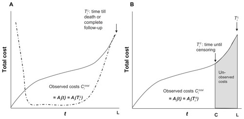
First, among the participants who die, death drives up costs in the period before death as seen in Figure 1A. Conversely, cumulative costs may in fact be driven down because no costs are accrued after death. The accepted method of dealing with this is to consider death as a terminal event.^7,9,11,12,18 Subjects will accrue costs until they die, or until they reach the time horizon of the analysis. A complete case is defined as one in which death occurs, or where follow-up is complete until the end of the restricted time period. In each of these situations, participants are no longer accumulating relevant costs.

The second issue is how to deal with the individuals who are not complete cases. A portion of the relevant health costs for these participants will be unobserved, as illustrated by the shaded area in Figure 1B.¹⁸ Such data are said to be right censored, defined as an observation that ends prematurely, before the outcome of interest has occurred (death or 1080 days, in the present example).¹⁸ Right censoring of health care costs can arise from a number of mechanisms. Patients may be lost to follow-up at varying times; alternatively, a study may enroll patients over a period of time but discontinue follow-up on a fixed calendar date. In both of these cases, the censoring occurs completely at random, and the observed health care costs represent the lower limit of the relevant costs. One way of adjusting cumulative cost estimates for censoring is to develop a function that describes the way in which data are censored and to use that function to reweight the observed cost data. Kaplan-Meier techniques are a well-established method to achieve such reweighting.

Kaplan-Meier estimates for survival and censoring

First, the traditional Kaplan-Meier estimator for survival will be reviewed, and then an analogous estimator for censoring will be introduced.¹² Please see Table 1 for explanation of the nomenclature in this section. A traditional Kaplan-Meier estimator, S(t) is the probability of surviving beyond a time, t. In this method, patients who are censored are no longer at risk for death and are therefore excluded. The probability of survival for any interval is equal to the proportion surviving among those still at risk of death at the beginning of the interval (ie, uncensored cases). The Kaplan-Meier estimator at time t is calculated by multiplying the probabilities of surviving each time interval preceding point t – hence, it is also referred to as the product-limit estimator.

Table 1 Nomenclature

Term	Definition
S(t)	Probability of being alive beyond time t
Sc(t)	Probability of being uncensored beyond time t
i	Individual
N	Total number of individuals in study
j	Cost interval (ie, 30 days)
K	Total number of costing intervals
Ci^total	Accumulated cost for individual i
ti	Period of observation for individual i
Ti^L	Time of observation until death/cure/end of relevant period for an individual who is considered a complete observation
Ti^C	Time of observation until censoring for an individual who is censored
Ai(ti)	The cost function used to estimate cumulative cost until time t for patient i
Mi^j	The total cost for each subinterval j for each patient i
R	Rate of cost accumulation

The Kaplan-Meier estimate for censoring, S_c(t), is defined as the probability for being uncensored beyond time t.¹² Here, the role of death and censoring are reversed relative to a conventional survival analysis. Censoring is the outcome of interest, and death simply means that the patient is excluded from further observations. The risk of being uncensored in a particular interval is calculated for those who are “at risk” of being censored at the beginning of the interval. These are the patients who have not been removed or excluded – that is, those who have not died or been censored. Again, S_c(t) for time t is the product of all probabilities of being uncensored across intervals prior to time t.

To illustrate these concepts, four hypothetical patients are presented in Table 2, followed over 6 months. Patients A and B are followed for all 6 months, while patient C dies in month 3 and patient D is censored in month 4. The components for both the Kaplan-Meier estimates for survival, S(t), and the Kaplan-Meier estimates for censoring conditional on being alive, S_c(t), are shown on the right of the Table 2. When calculating the Kaplan-Meier estimate for survival, it is necessary to determine the probability of death and of survival for each month. These are shown with the number of patients at risk at the beginning of the month in the denominator. Importantly, patients who are censored are removed from the denominator. For example, in the third month, four patients are at risk for death at the beginning of the month, with three alive at the end of the month (probability of survival is 3/4 = 0.75). In month 5, only two are at risk for death at the beginning of the interval, because one patient was censored in the previous month (probability of survival is 2/2 = 1). S(t) is the product across the months of the probability of survival: S(4) = 1*1*0.75*1 = 0.75.

Table 2 Hypothetical patient cohort to illustrate Kaplan-Meier techniques

Data					Survival			Censoring
Month	Patient A	Patient B	Patient C	Patient D	Probability of death within interval	Probability of survival within interval	S(t)	Probability of censoring within interval	Probability of being uncensored within interval	Sc(t)
1	x	x	x	x	0/4	4/4 = 1	1	0/4	4/4 = 1	1
2	x	x	x	x	0/4	4/4 = 1	1*1 = 1	0/4	4/4 = 1	1*1 = 1
3	x	x	Died	x	1/4	3/4 = 0.75	1*1*0.75 = 0.75	0/4	4/4 = 1	1*1*1 = 1
4	x	x		Censored	0/3	3/3 = 1	1*1*0.75*1 = 0.75	1/3	2/3 = 0.67	1*1*1*0.67 = 0.6 7
5	x	x			0/2	2/2 = 1	1*1*0.75*1*1 = 0.75	0/2	2/2 = 1	1*1*1*0.67*1 = 0.67
6	x	x			0/2	2/2 = 1	1*1*0.75*1*1*1 = 0.75	0/2	2/2 = 1	1*1*1*0.67*1*1 = 0.67

Notes: S(t) represents the Kaplan-Meier estimate for survival, defined as the probability of survival beyond time t; S _c(t) represents the Kaplan-Meier estimate for censoring, defined as the probability of being uncensored beyond time t, x, indicates that patient was observed in that month.

The corresponding calculations for S_c(t) are shown on the far right side of Table 2. Here, the denominator for each interval contains only patients at risk for censoring at the beginning of the interval; patients who died in the preceding interval are removed. For example, at the beginning of the fourth month, only three patients continue to be at risk for censoring. In the end of the fourth month, one patient was censored, so the probability of being uncensored is 2/3 = 0.67. The Kaplan-Meier estimate S_c(t) is the product across intervals of the probability of remaining uncensored: S_c(4) = 1*1*1*0.67 = 0.67.

In Figure 2A, the Kaplan-Meier survival curve is constructed from the HF study over a follow-up period of 1080 days, with the probability of survival, S(t), at the end of follow-up being 43%. It is evident that the probability of dying – the complement of S(t) – increases with larger values of t, after accounting for censoring.

Figure 2 (A) Kaplan-Meier survival curve (B) Kaplan-Meier curve for censoring

Notes: S(t) is probability of survival; S_c(t) is probability of being uncensored; t is follow-up time in days.

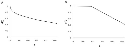
Over the full follow-up period of 1080 days, 14,107 patients of the original 43,888 patients were censored and therefore were no longer available for observation. In Figure 2B, the corresponding Kaplan-Meier curve is constructed, with the probability of being uncensored, S_c(t), decreasing at greater values of t. It is important to note that at greater values of time t, the probability of censoring increases – the complement of S_c(t).

Restricted time period total costs

First, the issues related to censoring in a restricted time period will be tackled. In order to understand the techniques, some nomenclature is necessary (see Table 1). Let N be the total sample size of the study, including both censored and uncensored cases. For each participant, i, there is an observed accumulated medical cost, denoted by C_i^total. Each individual has an observation time, denoted by t_i. For complete cases who are observed until death or until the end of the restricted time period, t_i is equal to the time to death/restricted time limit, denoted by T_i ^L. For a censored case, t_i is equal to the time to censoring, denoted by T_i ^C. Finally, an indicator variable is defined for each participant, Δ_i, which will take the value of 0 for censored cases and of 1 for complete cases. C_i^total for each participant will be expressed as a function A_i:

$C_i^{total}=A_i(t_i)$(1)

Each of these terms is illustrated in Figure 1A and B. Figure 1A shows the cumulative costs over time for a complete case, defined as a participant who is observed until T_i ^L. Figure 1B is a censored patient, observed only until the censoring time, T_i ^C. As illustrated by the shaded area, a censored patient will continue to accumulate relevant costs (ie, until T_i ^L) and these will be unobserved.

Full-sample and uncensored case estimators

Two potential estimators for mean restricted time total costs (C_i ^total) in the face of censored data are the full-sample and uncensored case estimators.^1,9,13 In the full-sample estimator, the accumulated cost for each participant is averaged, irrespective of whether the patient died, was observed for the full follow-up period, or was censored.^1,13 As censored patients will continue to accumulate relevant costs while unobserved (shaded portion in Figure 1B), the full-sample estimator would include only a portion of their relevant costs, and therefore it will always be an underestimate.¹

In the uncensored case estimator, only the values from complete cases are used.¹³ As illustrated in Figure 2B, the probability of remaining uncensored, S_c(t), is not uniform at all values of t. Instead, as t increases, the probability of being uncensored, S_c(t), decreases. Therefore, the uncensored case estimator would be biased toward the costs of participants who died early – those who had smaller values of t_i.^1,13

Reweighted estimators

One approach to estimate mean health care costs when censoring is present is to reweight each complete case so that each complete case represents not only itself but also some number of incomplete/censored cases. In this setting, the cumulative cost of each participant who died or reached the full period of observation must represent not only the cost of that participant but also the censored cases that would have been observed had there been no censoring. The number of censored cases that must be represented by a complete case at observation time t is proportional to the probability of that case being censored.^18,19 It follows that costs for complete cases with a short follow-up should be weighted less than cases with a longer observation period, accounting for the higher probability of censoring with longer observation periods.

Different reweighted estimators have been developed.^{1,9,13,18,20,21} These are conceptually similar and are equivalent under certain conditions.^12,21 The Lin 1997 estimator was the first to be described and is based on dividing observation time into a number of equal intervals.⁹ Lin et al⁹ described two alternative methods: one if cost histories are available, and a second if only total cumulative costs are available for all individuals. In the latter, more basic scenario, the mean cost for each interval is calculated, based only on the costs of patients who die during the interval. The cumulative cost for the entire period of observation is the sum of the mean costs for each interval, weighted by the Kaplan-Meier probability of surviving to the beginning of each interval.⁹ A limitation of the Lin 1997 estimator is the assumption of discrete censoring times that coincide with the beginning of the costing intervals.²² Bang and Tsiatis⁷ described an inverse probability weighted (IPW) estimator that did not require interval costs and which accommodated continuous censoring times. As an illustration, the IPW method of Bang and Tsiatis⁷ will be worked through in detail here. Interested readers are encouraged to refer to the source documentation for a full description of the other estimators, and for recommendations as to their appropriate use.^{1,9,12,13,18,20,21}

In the IPW estimator, sample weighting is done using the Kaplan-Meier estimate for censoring, S_c(t_i).^1,21 Each uncensored participant (Δ_i value of 1) with T_i^L of observation time has S_c(T_i ^L) probability of being uncensored, as seen in Figure 2B. Each uncensored observation represents on average 1/S_c(T_i ^L) patients who are censored (Δ_i value of 0).¹² Because uncensored observations are weighted by the inverse of S_c(t_i), it is apparent that patients who die early in the study (smaller values of t_i), and who therefore have smaller values of T_i ^L, are weighted less than those who die at longer follow-up times or who are followed up until the restricted time limit. The mean IPW total cost is estimated as:

$1/\text{N}[{\sum }_i^n{\mathrm{\Delta }}_i{A}_i(t_i)/S_c(t_i)]$(2)

Several key points from this merit discussion. Costs from all individuals are included, as N is the full sample. However, the costs of the censored participants are multiplied by the indicator variable of “0,” with only the costs of complete participants reweighted accordingly. An important limitation for this estimator is inefficiency, because only data from uncensored/complete cases inform the final value.¹³ Using simulation, Raikou and McGuire¹³ found that in the presence of very heavy censoring (>50%), the simple IPW estimator becomes unstable.

An alternative “partitioned estimator” is possible when cumulative cost histories are available for each participant. This is shown in Figure 3, where costs are available for subintervals of the full period of observation.¹² Censored patients are likely to have full costs for some of the subintervals. For example, in Figure 3, patient 2 is a complete case over the entire restricted time period (shaded area), and therefore patient 2 has complete costs for all four sub-intervals; patient 1 is censored in subinterval 3 but has full costs for subinterval 1 and 2 (shaded area). Because a censored patient is likely to have complete costs for some intervals, it is possible to make use of these data to further inform the estimator of mean cost.

Figure 3 Partitioned cost histories: the full period of observation is subdivided into four partitions. Patient 1 is censored in partition 3, while patient 2 is a complete case.

Notes: Shaded area represents partitions for patients 1 and 2, where full data is available; t is follow-up time.

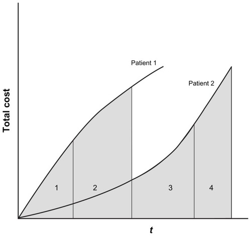
Bang and colleagues^7,21 developed a partitioned extension of their IPW estimator, in which the total time period is divided into K partitions or subintervals. For each subinterval, denoted as j, a participant will either be censored or have full observation, defined as dying within the subinterval or observation for the full subinterval. Thus, one can define variables Δ_i ^j, T_i ^C, T_i ^L, t_i ^j specific to each subinterval j of interest. M_i ^j designates the total cost for each subinterval j. M_i ^j is calculated as the difference between cumulative cost up to the end of the subinterval j and the cumulative cost in the preceding subinterval. This is given by the formula:

$M_i^j=[A_i^j(t_i^j)-A_i^{(j-1)}(t_i^{(j-1)})]$(3)

For illustration, in Figure 3, the cost for patient 1 for subinterval 2 is the difference between the entire shaded area – the first term in equation 4: A_i ^j(t_i ^j) – and the shaded area to the left of the line separating the first and second interval – the second term in equation 4: A_i ^(j−1)(ti^(j−1)). By summing the cost estimate for each subinterval, the mean total cost can be determined. The mean partitioned IPW estimator for total restricted time costs will then be:

$1/\text{N}[{\sum }_i^n{\sum }_j^K{\mathrm{\Delta }}_i^j{M}_i^j/S_c(t_i)]$(6)

Investigators have shown that the Lin 1997 method and the IPW estimator are equivalent when the intervals for the Lin 1997 method become infinitesimally small (ie, approach continuous censoring time).¹² In order to extend beyond estimation of the mean and make formal inferences, both the Lin 1997 and Bang-Tsiatis methods allow for the calculation of variances. These calculations are necessarily complex – readers are encouraged to review the source documentation on this area and are strongly encouraged to involve a statistician. Moreover, using the simple IPW or the partitioned IPW as response variables, these methods can be expanded within a regression framework to control for covariates.^10,11,18 However, the IPW techniques have a number of limitations, especially when evaluating covariate effects, as the effects on cost accumulation cannot be distinguished from the effects on survival.²² Moreover, these techniques do not account for the differential rates of heath care cost accumulation near death, as seen in Figure 1A and B. Alternative models have been developed to deal with these issues.²²

Simulations

The authors used a similar simulation method to Basu and Manning²² to generate a cohort of 1000 patients, evaluated over a maximum of ten equally spaced intervals. Patients who died or who completed observation until the end of the ten periods were considered to be complete observations. Survival and censoring times were generated from an exponential distribution and a uniform distribution, respectively.²² As per previous investigators, the present authors generated a cumulative cost profile for individuals, such that there was an increased initial cost reflecting diagnosis and an increased terminal cost in the event of death.

The authors used combinations of censoring and survival times to create datasets with increasing degrees of censoring. Using 500 simulations per dataset, the authors then compared a full-sample, uncensored, and simple IPW estimator with the true mean costs. These results are shown in Table 3.

Table 3 Simulations to evaluate impact of censoring

Censoring	Mean ten-interval cumulative costs ($)a	Interquartile range
7% Censoring
True costs	8.29	8.21–8.38
Full-sample estimator	7.49	7.41–7.56
Uncensored case estimator	7.68	7.61–7.77
Simple IPW	8.06	7.97–8.15
18% Censoring
True costs	8.29	8.20–8.37
Full-sample estimator	7.03	6.96–7.10
Uncensored case estimator	7.50	7.42–7.58
Simple IPW	8.49	8.39–8.59
21% Censoring
True costs	9.07	9.00–9.16
Full-sample estimator	7.57	7.49–7.65
Uncensored case estimator	8.20	8.12–8.28
Simple IPW	9.35	9.24–9.45
53% Censoring
True costs	7.45	7.37–7.53
Full-sample estimator	4.90	4.89–5.04
Uncensored case estimator	5.28	5.18–5.38
Simple IPW	9.87	9.64–10.1

Note:

a Costs adjusted to 2008 Canadian dollars using the Bank of Canada consumer price index (http://www.bankofcanada.ca/en/cpi.html).

Abbreviation: IPW, inverse probability weighting.

As expected, with increasing censoring, the full-sample estimator underestimated the true costs. The simple IPW estimator performed well with mild to moderate degrees of censoring in the simulated datasets; however, with heavy censoring (53%) it substantially overestimated true costs. This is consistent with reports with other investigators as to its instability in the presence of high censoring.

HF case study

Using data from the 43,888 patients in the HF case study, the authors calculated estimators for the mean 1080-day total cost. Cost histories were available for 180-day partitions. Statistical models were created using R software (v 2.9.0; R Foundation for Statistical Computing, Vienna, Austria) and are available upon request. Of the 43,888 patients, 32.1% were censored over the 1080-day restricted time period, with 50.9% of patients dying and 17% having complete follow-up to 1080 days. In Table 4, the full-sample estimator, uncensored case estimator, simple IPW estimator, and the partitioned 180-day estimator are shown. In addition, the authors estimated costs using the Lin 1997 method based on total accumulated costs. Two versions of the Lin 1997 method, using 180- and 30-day intervals, were utilized to highlight issues that may arise from the choice of time-interval.

Table 4 Mean 1080-day costs using different estimating methods

Estimating method	Mean 1080-day cumulative costs ($)a	Interquartile range
Full-sample estimator	30,420	10,060–37,850
Uncensored case estimator	33,940	11,480–42,890
Simple IPW	36,490	0–44,620
Partitioned IPW	33,230	10,260–40,550
Lin 1997 (180-day interval)	20,059	NAb
Lin 1997 (30-day interval)	37,042	NAb

Notes:

a Costs adjusted to 2008 Canadian dollars using the Bank of Canada consumer price index (http://www.bankofcanada.ca/en/cpi.html);

b the Lin 1997 method produces a single mean value for the sample, as opposed to a reweighted estimate for each individual – as such, an interquartile range is not available.

Abbreviations: NA, not applicable; IPW, inverse probability weighting.

As anticipated, the full-sample estimator was the lowest, at $30,420 for the 3-year (1080-day) period, which is a biased underestimate. A total of 14,107 patients were censored within the restricted time period and had costs that would have otherwise accrued in the absence of censoring (ie, the shaded portion in Figure 2B). The uncensored estimate is higher, at $33,940, and disproportionately biased patients with short survival times, who in this dataset have higher costs. The simple IPW cost of $36,490 only makes use of the 67.2% of data not censored. With the partitioned IPW estimator, which makes use of data from all the subjects, the estimate for mean 1080-day cumulative cost was $33,230. In contrast, the Lin 1997 method, based on intervals of 180 days, provides a substantially lower mean estimate of $20,059, while the Lin 1997 estimate using a 30-day interval of $37,042 closely approximated the simple IPW estimate. This highlights the differences between the Lin 1997 methods and the IPW estimator when longer time intervals are used.

Lifetime costs

Although using a restricted time period allows one to circumvent the issue of extrapolating lifetime costs and is often used in practice, a restricted time period cost has important limitations. ¹⁸ For example, two patients may have the same lifetime cumulative costs but because of differences in survival times (ie, one patient dies at 3 years and the other dies at 5 years), may have substantially different time-restricted costs at 3 years.¹⁸ When studying interventions with significant influences on mortality, having the same distribution of lifetime costs in the control and study groups is not synonymous with having the same distribution of time-restricted costs, because the survival distributions in the groups may be different.

Given the critical relationship between survival time and health care costs, it is tempting to use Kaplan-Meier techniques, substituting time to death with cost to death as the dependent variable. However, investigators have found that this results in biased estimates.^3,8,18,23 A fundamental requirement for a Kaplan-Meier survival curve is independent censoring.^3,8,18,23 For survival time, this requires that the time to censoring is independent of the time to death. In most cases this is true; however, in the parallel form for costs, the cumulative cost to censoring for a particular participant will not be independent from the cumulative costs to death because both are related to the participant’s unique pattern of cost accumulation (Figure 1A).^3,8,18,23 This is most obvious in the situation of a constant rate of cost accumulation, R, where the cumulative cost at censoring time, T_i ^C, is simply the product of R*T_i ^C, while that at time of death, T_i ^L, is R*T_i ^L. Both values are clearly not independent but are related to each other by R.^3,8,18,23

Phase-based costing

An alternative method for estimating cumulative costs is using is a phase-based modeling approach.^14,24–26 This is particularly attractive for estimating lifetime costs or cost in the presence of heavy censoring. The steps for the phase-based approach are as follows:^14,24–26

1. Define a priori clinically important phases of disease. Examples are the phase immediately after diagnosis, associated with higher costs; a stable phase, with constant and low costs; and the phase prior to death, which again has high costs.

2. Determine inflection points in cumulative cost, which define the duration of each phase. This will be disease specific.

3. Allocate observation time and costs for each patient to the phases.

4. Once the costs for all patients have been assigned, determine the mean cost per phase (or per subdivision of each phase).

5. Using both the data on cost per phase and time to death, determine the cumulative lifetime costs.

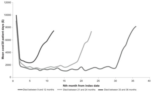
Each of these steps will now be worked through in the HF example. First, based on content experts, the authors expected that HF would be characterized by at least three phases: (1) a post-discharge phase after index hospitalization, (2) a pre-death phase, and (3) a relatively stable phase (Step 1). To confirm this hypothesis, the authors evaluated the cost per 30 days for patient subgroups that survived 9–12, 21–24, and 33–36 months post discharge (Appendix Figure 1). The mean 30-day cost curves confirmed the hypothesis of discrete cost phases with inflection points separating the post-discharge and stable phases, and the stable and pre-death phases estimated at 3 months post discharge and 6 months prior to death, respectively (Step 2).

Figure A1 Exploratory analysis on phases of long-term cost^a associated with heart failure care.

Note: ^aCosts adjusted to 2008 Canadian dollars using the Bank of Canada consumer price index (http://www.bankofcanada.ca/en/cpi.html).

The cumulative cost history for each individual over the 1080-day period of the study was partitioned and sequentially allocated to phases (Step 3). For example, for each patient the cumulative costs for the first 3 months of observation were assigned to the post-diagnosis phase, the costs associated with the 6 months prior to death were assigned to the predeath phase, and the remainder were assigned to the stable phase. Once the entire cohort was analyzed in this manner, a mean cost was calculated for each of the phases (Step 4). In the present study, the mean costs were determined for each 30-day block within each phase (Appendix Table 1). Other investigators have used a simpler approach in which a single mean cost is determined per phase.²⁷ It is important to note that costs should be adjusted to the current year in order to account for health care inflation, using a multiplier such as the consumer price index.

Table A1 Phase-based costing example using heart failure cohort

30-day block	Observed costs ($)a
Post-discharge phase
Block 1	10,675
Block 2	2961
Block 3	2172
Stable phase
All blocks	617
Pre-death phase
Block 6	3062
Block 5	3501
Block 4	4077
Block 3	5119
Block 2	8716
Block 1	8308
Mean lifetime cost	61,870

Note:

a Costs adjusted to 2008 Canadian dollars using the Bank of Canada consumer price index (http://www.bankofcanada.ca/en/cpi.html).

To calculate cumulative costs, one utilizes both the mean costs per phase and a survival function that spans the time horizon of the study (lifetime or shorter) (Step 5). Although the survival and cost data are from the same cohort in the earlier techniques, this need not be the case in the phase-based approach.²⁸ In the present study, the authors used a survival curve from a separate HF cohort that had been followed for 12 years, over which period 99% of patients died.

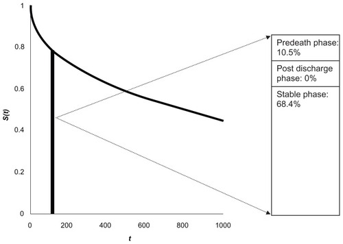
First, the survival curve is divided into intervals. In the present example the authors used 30-day time intervals. For any time interval on the survival curve, the proportion of the original cohort in each phase is determined. This proportion is multiplied by the mean cost for that particular phase. In Figure 4, for example, at the 120- to 150-day time interval on the survival curve, 68.4% of the original HF cohort were in the stable phase – the cost for this phase was 0.684*$617 = $422. None of the patients were in the postdischarge phase, and 10.5% were in the pre-death phase (for a cost of $614). Thus, the cost for t = 120- to 150-day interval is $422 + $614 = $1036. The costs for all time intervals are calculated in this manner and are summed to produce the mean cost for the entire time horizon.

Figure 4 Merging phase-based costs on the survival curve. For the time interval 120–150 days, 68.4% of the original cohort was in the stable phase, with 10.5% in the pre-death phase. To determine the cost for the time interval of 120–150 days, the proportion of patients in each phase is multiplied by the mean cost per phase, as shown in Appendix Table A1.

Notes: S(t) is probability of survival; t is follow-up time in days.

The authors found that over a mean life expectancy of 3.87 years, HF patients had a mean lifetime cost of $61,870.¹⁴ To provide a comparison with the methods already mentioned, the authors also calculated the mean cost at 1080 days, using a phase-based approach. The phase-based estimate of $37,237 was similar to that from the other methods – specifically, the simple IPW and the Lin 1997 methods.

Data comparing such phase-based estimates with those from IPW methods are sparse, but with investigators to date finding that they are comparable.²⁶ The benefits of the phase-based approach are that actual costs for the cohort over the entire period of interest (ie, lifetime) do not need to be observed, thereby overcoming the major limitation of the previous methods.^14,24–26 Using these methods, investigators have been able to produce widely used estimates of the lifetime costs of cancer.^26,29 However, greater understanding of when one technique is favored over another is important and should be a focus for further methodological study.

Conclusion and recommendations

This review has provided an overview for the uninitiated reader who wishes to tackle the literature on health care costing with data that are incomplete because of incomplete follow-up. The authors offer the following recommendations:

1. Censoring will have substantial methodological impact on a study, and investigators must evaluate their data to determine if any cases are right censored.

2. If censoring is present, the use of either a full-sample estimator or an uncensored case estimator in the estimation of mean cost is potentially inaccurate.

3. The choice of estimator when censoring is present is not clear-cut. Options include a weighted estimator (preferably a partitioned estimator, to make use of all the data efficiently) or a phase-based approach.

Given the importance of health care costing for comparative effectiveness research and in the shaping of future health policy, the authors believe that further work on developing accurate yet transparent techniques should be a priority; the authors’ hope is that this review serves as a stimulus for such work.

Disclosure

The authors report no conflicts of interest in this work.

Appendix