Attributing diseases to multiple pathways: a causal-pie modeling approach

Abstract

Characterizing the relations between exposures and diseases is the central tenet of epidemiology. Researchers may want to evaluate exposure-disease causation by assessing whether the disease under concern is induced by the various exposures – the so-called “attribution”. In this paper, the authors propose a method to attribute diseases to multiple pathways based on the causal-pie model. The method can also be used to evaluate the potential impact of an intervention strategy and to allocate responsibility in tort-law liability issues.

Keywords:

• epidemiological methods
• attribution
• disease pathways
• causal-pie model

Introduction

Characterizing the relations between exposures and diseases is the central tenet of epidemiology. Epidemiologists may be interested in knowing the influence of a single exposure on a disease (using effect measures such as risk difference, risk ratio, and odds ratio) or the total influence of multiple exposures on the disease. They may also be interested in knowing any possible interaction between exposures. Through epidemiological studies, the complex relations between multiple exposures and a disease can be clarified.¹

Attention has also been given to the “processes”, “pathways”, or “mechanisms” themselves, through which an exposure brings about the disease. For example, one may want to know whether the causal relationship between an exposure and a disease is mediated by a specific “mediator”. If so, the influence of the exposure on the disease can be decomposed: the “indirect effect” is the effect mediated by the mediator, and the “direct effect” is the one not mediated by it. A statistical method that can decompose the exposure effect is structural equation modeling (SEM).^2–4 Effect decomposition in SEM is straightforward; the effect pertaining to a specific pathway is simply the product of the path coefficients of the traveled paths. For the indirect effect, we sum up the effects of those pathways that pass through the mediator, and for the direct effect, those that do not pass through it. However, this only works for a continuous mediator and continuous disease. The methods proposed by Robins and Greenland,⁵ Pearl,⁶ and VanderWeele⁷ are more general. These methods can accommodate any variable type and can cope with exposure–mediator interactions and nonlinear relations between variables.

The aforementioned methods evaluate exposure–disease causation by going from exposures to a disease. Sometimes we may be interested in backward induction by assessing whether the disease under concern is induced by the various exposures – the so-called “attribution”. (Note that the attribution here is based on epidemiologic data,^8–14 and should not be confused with attribution in social psychology where the human perception of causations is in focus.)¹⁵ For example, when planning intervention strategies, policymakers may want to compare the effectiveness of various intervention programs directed at removing different exposures in the population. In this case, we need to know the proportion of disease that was induced by each exposure. As another example, in some tort litigation, the court is concerned about the contribution of a specific exposure to the disease occurrence of the plaintiff. If probabilistic apportionment of causal responsibility^16,17 is adopted, the court needs to know the probability that the occurrence of the disease was induced by this exposure. In situations like these, we can use indices such as the attributable fraction^8–12 and the causal-pie weight^13,14 for attribution. When there are multiple exposures, a summation of the attributable fractions for all exposures may exceed 100%. Clearly, this makes no sense, and the index needs some rectifications.^18–23 When there are multiple exposures, one can compute a panel of causal-pie weights (summing up to 100%) for the individual effects of each and every exposure as well as the interactive effects between them. However, neither the attributable fraction nor the causal-pie weight takes disease pathways into account.

In this paper, we propose a method to attribute diseases to multiple pathways based on the causal-pie model.^1,24 The method can also be used to evaluate the potential impact of an intervention strategy and to allocate responsibility in tort-law liability issues.

Methods

Relations between an exposure, a mediator, and a disease

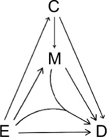
A “directed acyclic graph” (DAG)^1,25,26 is used to depict the causal relations between an exposure (E) and a disease (D), which can be mediated by a mediator (M) (Figure 1). Causality (also referred to as causation, or cause and effect) is a process (arrows in Figure 1) that connects one set of variables (the “causes” or “risk factors”) with another set of variables (the “effects” or “outcomes”), where the first is partly responsible for the second, and the second is partly dependent on the first. An effect (outcome) can, in turn, be a cause (risk factor) for many other effects (outcomes). Note that a DAG depicts a simplified biology, ignoring any feedback loop where an effect can feed back to the same cause that leads to the very effect in the first place.

Figure 1 The two paths for M-stage and four paths for D-stage.

Abbreviations: D, disease; E, exposure; M, mediator.

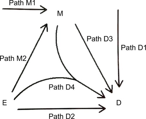
We consider the exposure, the disease, and the mediator as dichotomous variables. We call the occurrence of the mediator, the M-stage, such as the paths M1 and M2, and the occurrence of the disease, the D-stage, such as the paths D1, D2, D3, and D4 (Figure 1). Note that to indicate “interaction”, we allow two DAG arrows to meet and merge before pointing at the same variable, such as the D4 path in Figure 1.

A causal-pie model for mediator and disease

We follow the causal-pie framework for mediator and disease proposed by Hafeman.²⁷ We invoke the “sufficient-cause positive monotonicity assumption” at the individual level, that is, the effects of the exposure on the mediator and on the disease as well as the effect of the mediator on the disease, if any, can only be harmful and cannot be preventive for any individual.^{1,13,14,27,28} In Figure 2, under the assumption, there is a total of six classes of causal pies – two for the M-stage and four for the D-stage. The two causal-pie classes for the M-stage are: 1) a causal-pie class not containing E as its component and 2) a causal-pie class containing E as its component (1 and 2 correspond to paths M1 and M2 in Figure 1, respectively). The four causal-pie classes for the D-stage are: 3) a causal-pie class containing neither E nor M as its component, 4) a causal-pie class containing E but not M as its component, 5) a causal-pie class containing M but not E as its component, and 6) a causal-pie class containing both E and M as its components (3, 4, 5, and 6 correspond to paths D1, D2, D3, and D4 in Figure 1, respectively).

Figure 2 The total six causal-pie classes for M-stage and D-stage.

Notes: (A) M-stage; (B) D-stage.
Abbreviations: D, disease; E, exposure; M, mediator; U, unknown components.

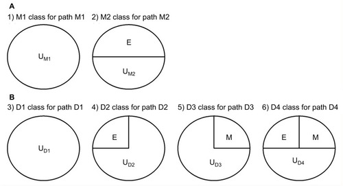
Aside from the exposure and the mediator, each causal-pie class contains a distinct constellation of unknown components. We denote these by U – the U_M1, U_M2, U_D1, U_D2, U_D3, and U_D4, respectively, in Figure 2. When all components in a causal pie appear, the causal pie is completed, and the corresponding mediator or disease is meant to occur. The arrivals of the unknown components (U) are random events. When the U of a particular causal pie arrives and other component(s) (E, M, or both), if any, in the causal pie all exists, the causal pie is completed, and as mentioned previously, the corresponding mediator or disease occurs. Otherwise, the U departs, and the completion of this causal pie is contingent on the events that the same U arrives again.

Disease pathways

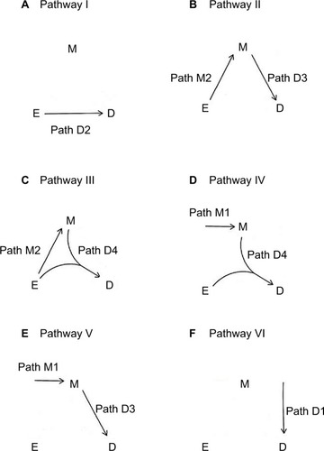
An individual can follow the paths depicted in Figure 1 to become diseased. A total of six distinct disease pathways can thus be identified (Figure 3):

1. I. The exposure causes the disease directly (D2).

2. II. The exposure causes the mediator, which in turn causes the disease (M2D3).

3. III. The exposure causes the mediator, and then both interact to cause the disease (M2D4).

4. IV. The exposure and an exogenous mediator interact to cause the disease (M1D4).

5. V. An exogenous mediator causes the disease directly (M1D3).

6. VI. Neither the exposure nor the mediator causes the disease (D1).

Note that these pathways are examined at the individual level rather than population, that is, the same person is followed-up throughout for the path(s) he/she had actually taken to eventually become diseased. Therefore, we can distinguish the actual “operation” from the mere “presence” of a mediator.^29,30 Pathways IV and V (Figure 3) only imply the presence of an “M” in the disease pathway. On the other hand, Pathways II and III (Figure 3) not only imply the presence of the M but also its operation (a person goes from E to M, and then to D), and the M now can truly be called a “mediator”.

Figure 3 The six disease pathways.

Notes: (A) Pathway I; (B) Pathway II; (C) Pathway III; (D) Pathway IV; (E) Pathway V; (F) Pathway VI.
Abbreviations: D, disease; E, exposure; M, mediator.

Estimation of the causal-pie parameters

We assume that in the follow-up period, the arrival rates of U in the six classes of causal pies, denoted by λ_M1, λ_M2, λ_D1, λ_D2, λ_D3, and λ_D4, respectively, are constant. We also invoke the “no redundancy assumption”,^28,31,32 that is, for each and every subject in the population, at most one U can arrive in a sufficiently short time interval.

One can conduct a cohort study to estimate the aforementioned six causal-pie parameters – λ_M1, λ_M2, λ_D1, λ_D2, λ_D3, and λ_D4. Suppose that there are n exposed subjects and m unexposed subjects in the cohort. At the start of the follow-up (t=0), all the subjects are mediator- and disease-free. During the follow-up period (from t=0 to t=T), for subjects who contracted the disease, the researcher records their mediator status at the moments they contracted the disease. For subjects who did not contract the disease during the following period, the researcher records their mediator status at the end of the follow-up (t=T). A tally of subjects at the end of the follow-up is shown in Table 1. This dataset has a total of 6 degrees of freedom (2² − 1=3 for the exposed subjects and 2² − 1=3 for the unexposed), which is equal to the number of the unknown parameters. Therefore, λ_M1, λ_M2, λ_D1, λ_D2, λ_D3, and λ_D4 are just identifiable. See Supplementary materials for details of the estimation procedure.

Table 1 A tally of subjects at the end of the follow-up of a cohort study

Mediator status and disease status	Exposure status
	E=0	E=1
M=0, D=0	m1	n1
M=1, D=0	m2	n2
M=0, D=1
M=1, D=1
Total	m = m1 + m2 + m3 + m4	n = n1 + n2 + n3 + n4

Notes: Inside the box are the diseased subjects. n and m represent number of subject.

Abbreviations: D, disease; E, exposure; M, mediator.

Attribution, a backward induction process

As pointed out earlier, attribution is a backward induction process, assessing whether the outcome under concern is induced by some variables. Thus, we reverse the direction of the usual DAG arrows in Figure 1 to become the “attribution arrows” (Figures 4 and 5). When an attribution arrow points at a variable (exposure or mediator), it means that the indicated variable is one cause of the outcome (disease or mediator, depending on the point from which the arrow originates). When an attribution arrow points at the exposure and the mediator simultaneously, it means that the exposure and the mediator interact to cause the disease. When an attribution arrow points at nothing, it means that neither the exposure nor the mediator is a cause of the disease (or the mediator).

Figure 4 Formulae for attribution.

Abbreviations: D, disease; E, exposure; M, mediator.

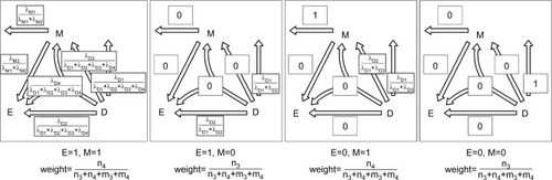
Figure 5 Disease attributions for the example cohort.

Abbreviations: D, disease; E, exposure; M, mediator.

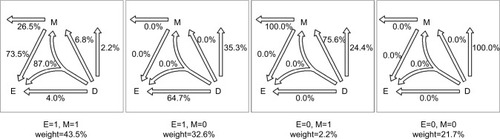
Given the six causal-pie parameters, we can compute the probability for any path (Figure 4). Consider the M-stage first (begin with the “M” in Figure 4 and follow the attribution arrows), an unexposed subject who acquires the mediator during the follow-up can only acquire it through path M1 (probability=1) but not path M2 (probability=0). An exposed subject who acquires the mediator can acquire it either through path M1 or M2, but not both (because of the no redundancy assumption). By Bayes theorem (Supplementary materials), the probabilities are $\frac{{\mathrm{\lambda }}_{\mathrm{M}1}}{{\mathrm{\lambda }}_{\mathrm{M}1}+{\mathrm{\lambda }}_{\mathrm{M}2}}$ (path M1) and $\frac{{\mathrm{\lambda }}_{\mathrm{M}2}}{{\mathrm{\lambda }}_{\mathrm{M}1}+{\mathrm{\lambda }}_{\mathrm{M}2}}$ (path M2), respectively. Next, consider the D-stage (begin with the “D” in Figure 4 and follow the attribution arrows) and also apply the Bayes theorem. An unexposed subject who acquires the disease but not the mediator during the follow-up can do so only through path D1 (probability=1). An unexposed subject who acquires the disease and the mediator can take either path D1 or D3 (with probabilities $\frac{{\mathrm{\lambda }}_{\mathrm{D}1}}{{\mathrm{\lambda }}_{\mathrm{D}1}+{\mathrm{\lambda }}_{\mathrm{D}3}}$ and $\frac{{\mathrm{\lambda }}_{\mathrm{D}3}}{{\mathrm{\lambda }}_{\mathrm{D}1}+{\mathrm{\lambda }}_{\mathrm{D}3}}$, respectively). An exposed subject who acquires the disease but not the mediator can take either path D1 or D2 (with probabilities $\frac{{\mathrm{\lambda }}_{\mathrm{D}1}}{{\mathrm{\lambda }}_{\mathrm{D}1}+{\mathrm{\lambda }}_{\mathrm{D}2}}$ and $\frac{{\mathrm{\lambda }}_{\mathrm{D}2}}{{\mathrm{\lambda }}_{\mathrm{D}1}+{\mathrm{\lambda }}_{\mathrm{D}2}}$, respectively). An exposed subject who acquires the disease and the mediator can take either path D1, D2, D3, or D4 (with probabilities $\frac{{\mathrm{\lambda }}_{\mathrm{D}1}}{{\mathrm{\lambda }}_{\mathrm{D}1}+{\mathrm{\lambda }}_{\mathrm{D}2}+{\mathrm{\lambda }}_{\mathrm{D}3}+{\mathrm{\lambda }}_{\mathrm{D}4}}$, $\frac{{\mathrm{\lambda }}_{\mathrm{D}2}}{{\mathrm{\lambda }}_{\mathrm{D}1}+{\mathrm{\lambda }}_{\mathrm{D}2}+{\mathrm{\lambda }}_{\mathrm{D}3}+{\mathrm{\lambda }}_{\mathrm{D}4}}$, $\frac{{\mathrm{\lambda }}_{\mathrm{D}3}}{{\mathrm{\lambda }}_{\mathrm{D}1}+{\mathrm{\lambda }}_{\mathrm{D}2}+{\mathrm{\lambda }}_{\mathrm{D}3}+{\mathrm{\lambda }}_{\mathrm{D}4}}$, and $\frac{{\mathrm{\lambda }}_{\mathrm{D}4}}{{\mathrm{\lambda }}_{\mathrm{D}1}+{\mathrm{\lambda }}_{\mathrm{D}2}+{\mathrm{\lambda }}_{\mathrm{D}3}+{\mathrm{\lambda }}_{\mathrm{D}4}}$, respectively).

Now we can compute the probability for any pathway. First, we note that under the no redundancy assumption, no one can acquire the disease and the mediator at the same time. A subject who acquires both the disease and the mediator during the follow-up must acquire the mediator before acquiring the disease. To calculate the probability for a pathway that straddles an M-stage path and a D-stage path, we simply multiply the two corresponding probabilities for the two paths. Following this multiplication rule, we can attribute the disease to multiple pathways probabilistically for a diseased subject with known exposure and mediator status. For a subject with unknown exposure and/or mediator status or for all the diseased subjects in the population, we can use the cell counts inside the box in Table 1 as the weights (shown underneath each panel in Figure 4) for attribution.

Next, we discuss attribution from three different perspectives: 1) attributing diseases to multiple pathways, 2) evaluating the potential impact of an intervention strategy, and 3) allocating responsibility in tort-law liability issues.

Attributing diseases to multiple pathways

We can attribute the diseases in the population to the aforementioned six pathways. The population attributable fractions (PAF), which take into account all the diseased subjects in the population, are: $\begin{array}{l}{\text{PAF}}_{\mathrm{I}}=\frac{{\mathrm{n}}_4}{{\mathrm{n}}_3+{\mathrm{n}}_4+{\mathrm{m}}_3+{\mathrm{m}}_4}\times \frac{{\mathrm{\lambda }}_{\mathrm{D}2}}{{\mathrm{\lambda }}_{\mathrm{D}1}+{\mathrm{\lambda }}_{\mathrm{D}2}+{\mathrm{\lambda }}_{\mathrm{D}3}+{\mathrm{\lambda }}_{\mathrm{D}4}}+\\ \frac{{\mathrm{n}}_3}{{\mathrm{n}}_3+{\mathrm{n}}_4+{\mathrm{m}}_3+{\mathrm{m}}_4}\times \frac{{\mathrm{\lambda }}_{\mathrm{D}2}}{{\mathrm{\lambda }}_{\mathrm{D}1}+{\mathrm{\lambda }}_{\mathrm{D}2}},\end{array}$(1) $\begin{array}{l}{\text{PAF}}_{\text{II}}=\frac{{\mathrm{n}}_4}{{\mathrm{n}}_3+{\mathrm{n}}_4+{\mathrm{m}}_3+{\mathrm{m}}_4}\times \frac{{\mathrm{\lambda }}_{\mathrm{D}3}}{{\mathrm{\lambda }}_{\mathrm{D}1}+{\mathrm{\lambda }}_{\mathrm{D}2}+{\mathrm{\lambda }}_{\mathrm{D}3}+{\mathrm{\lambda }}_{\mathrm{D}4}}\times \\ \frac{{\mathrm{\lambda }}_{\mathrm{M}2}}{{\mathrm{\lambda }}_{\mathrm{M}1}+{\mathrm{\lambda }}_{\mathrm{M}2}},\end{array}$(2) ${\text{PAF}}_{\text{III}}=\frac{{\mathrm{n}}_4}{{\mathrm{n}}_3+{\mathrm{n}}_4+{\mathrm{m}}_3+{\mathrm{m}}_4}\times \frac{{\mathrm{\lambda }}_{\mathrm{D}4}}{{\mathrm{\lambda }}_{\mathrm{D}1}+{\mathrm{\lambda }}_{\mathrm{D}2}+{\mathrm{\lambda }}_{\mathrm{D}3}+{\mathrm{\lambda }}_{\mathrm{D}4}}\times \frac{{\mathrm{\lambda }}_{\mathrm{M}2}}{{\mathrm{\lambda }}_{\mathrm{M}1}+{\mathrm{\lambda }}_{\mathrm{M}2}},$(3) ${\text{PAF}}_{\text{IV}}=\frac{{\mathrm{n}}_4}{{\mathrm{n}}_3+{\mathrm{n}}_4+{\mathrm{m}}_3+{\mathrm{m}}_4}\times \frac{{\mathrm{\lambda }}_{\mathrm{D}4}}{{\mathrm{\lambda }}_{\mathrm{D}1}+{\mathrm{\lambda }}_{\mathrm{D}2}+{\mathrm{\lambda }}_{\mathrm{D}3}+{\mathrm{\lambda }}_{\mathrm{D}4}}\times \frac{{\mathrm{\lambda }}_{\mathrm{M}1}}{{\mathrm{\lambda }}_{\mathrm{M}1}+{\mathrm{\lambda }}_{\mathrm{M}2}},$(4) $\begin{array}{l}{\text{PAF}}_{\mathrm{V}}=\frac{{\mathrm{n}}_4}{{\mathrm{n}}_3+{\mathrm{n}}_4+{\mathrm{m}}_3+{\mathrm{m}}_4}\times \frac{{\mathrm{\lambda }}_{\mathrm{D}3}}{{\mathrm{\lambda }}_{\mathrm{D}1}+{\mathrm{\lambda }}_{\mathrm{D}2}+{\mathrm{\lambda }}_{\mathrm{D}3}+{\mathrm{\lambda }}_{\mathrm{D}4}}\times \\ \frac{{\mathrm{\lambda }}_{\mathrm{M}1}}{{\mathrm{\lambda }}_{\mathrm{M}1}+{\mathrm{\lambda }}_{\mathrm{M}2}}+\frac{{\mathrm{m}}_4}{{\mathrm{n}}_3+{\mathrm{n}}_4+{\mathrm{m}}_3+{\mathrm{m}}_4}+\frac{{\mathrm{\lambda }}_{\mathrm{D}3}}{{\mathrm{\lambda }}_{\mathrm{D}1}+{\mathrm{\lambda }}_{\mathrm{D}3}},\end{array}$(5) and $\begin{array}{l}{\text{PAF}}_{\text{VI}}=\frac{{\mathrm{n}}_4}{{\mathrm{n}}_3+{\mathrm{n}}_4+{\mathrm{m}}_3+{\mathrm{m}}_4}\times \frac{{\mathrm{\lambda }}_{\mathrm{D}1}}{{\mathrm{\lambda }}_{\mathrm{D}1}+{\mathrm{\lambda }}_{\mathrm{D}2}+{\mathrm{\lambda }}_{\mathrm{D}3}+{\mathrm{\lambda }}_{\mathrm{D}4}}+\\ \frac{{\mathrm{n}}_3}{{\mathrm{n}}_3+{\mathrm{n}}_4+{\mathrm{m}}_3+{\mathrm{m}}_4}\times \frac{{\mathrm{\lambda }}_{\mathrm{D}1}}{{\mathrm{\lambda }}_{\mathrm{D}1}+{\mathrm{\lambda }}_{\mathrm{D}2}}+\\ \frac{{\mathrm{m}}_4}{{\mathrm{n}}_3+{\mathrm{n}}_4+{\mathrm{m}}_3+{\mathrm{m}}_4}\times \frac{{\mathrm{\lambda }}_{\mathrm{D}1}}{{\mathrm{\lambda }}_{\mathrm{D}1}+{\mathrm{\lambda }}_{\mathrm{D}3}}+\frac{{\mathrm{m}}_3}{{\mathrm{n}}_3+{\mathrm{n}}_4+{\mathrm{m}}_3+{\mathrm{m}}_4},\end{array}$(6) for Pathways I, II, …, VI, respectively. It is worth noting that the six PAFs sum to one.

Evaluating the potential impact of an intervention strategy

We now consider the impact of a specific intervention. We note that if an intervention can block a segment of a pathway (for example, either path M2 or D3, but not necessarily both, of Pathway II), the whole pathway is blocked. To calculate the impact fraction for an intervention, we sum the PAFs for those pathways that are blocked by this intervention.

The impact fractions for a number of interventions are detailed: 1) a complete removal of the exposure from the population: this would block paths M2, D2, and D4 and therefore Pathways I, II, III, and IV. The impact fraction for this intervention is PAF_I + PAF_II + PAF_III + PAF_IV. 2) A complete obstruction of the exposure effect on the mediator: this would block path M2 and therefore Pathways II and III. The impact fraction for this intervention is PAF_II + PAF_III. 3) A complete obstruction of the mediator effect on the disease: this would block paths D3 and D4 and therefore Pathways II, III, IV, and V. The impact fraction of this intervention is PAF_II + PAF_III + PAF_IV + PAF_V.

Allocating responsibility in tort-law liability issues

As pointed out earlier, if probabilistic apportionment of causal responsibility is adopted for tort-law liability issues,^16,17 the court needs to know the probability that the occurrence of the disease was induced by the particular exposure. We can follow the attribution arrow(s) of a pathway and examine whether the arrow points at the exposure to decide whether the exposure is involved in the pathway. If the attribution arrow of the disease points at the exposure and the mediator simultaneously, the probability that the exposure is involved is taken to be 0.5 (since there is no further information about which path is more likely to be actually taken). But when the attribution arrow of the mediator points again at the exposure, it is then known for certain that the exposure is involved somewhere in the causal chain. Using these rules, the full attributable fractions for Pathways I, II, and III, a half of the attributable fraction for Pathway IV, and none for Pathways V and VI are allocated to the exposure, respectively.

To be precise, for an exposed subject who contracts the disease, the contribution of the exposure to his/her disease – the “attributable fraction among the exposed” (AFE) – is as follows: 1) if the subject does not acquire the mediator during the follow-up (the “E=1, M=0” panel in Figure 4), $\begin{array}{l}{\text{AFE}}^{\mathrm{M}=0}={\text{AFE}}_{\mathrm{I}}^{\mathrm{M}=0}+{\text{AFE}}_{\text{II}}^{\mathrm{M}=0}+{\text{AFE}}_{\text{III}}^{\mathrm{M}=0}+{\text{AFE}}_{\text{IV}}^{\mathrm{M}=0}\times 0.5\\ =\frac{{\mathrm{\lambda }}_{\mathrm{D}2}}{{\mathrm{\lambda }}_{\mathrm{D}1}+{\mathrm{\lambda }}_{\mathrm{D}2}}+0+0+0\times 0.5\\ =\frac{{\mathrm{\lambda }}_{D2}}{{\mathrm{\lambda }}_{\mathrm{D}1}+{\mathrm{\lambda }}_{\mathrm{D}2}};\end{array}$(7) 2) if the subject acquires the mediator during the follow-up (the “E=1, M=1” panel in Figure 4), $\begin{array}{l}{\text{AFE}}^{\mathrm{M}=1}={\text{AFE}}_{\mathrm{I}}^{\mathrm{M}=1}+{\text{AFE}}_{\text{II}}^{\mathrm{M}=1}+{\text{AFE}}_{\text{III}}^{\mathrm{M}=1}+{\text{AFE}}_{\mathrm{V}}^{\mathrm{M}=1}\times 0.5\\ =\frac{{\mathrm{\lambda }}_{\mathrm{D}2}}{{\mathrm{\lambda }}_{\mathrm{D}1}+{\mathrm{\lambda }}_{\mathrm{D}2}+{\mathrm{\lambda }}_{\mathrm{D}3}+{\mathrm{\lambda }}_{\mathrm{D}4}}+\frac{{\mathrm{\lambda }}_{\mathrm{D}3}}{{\mathrm{\lambda }}_{\mathrm{D}1}+{\mathrm{\lambda }}_{\mathrm{D}2}+{\mathrm{\lambda }}_{\mathrm{D}3}+{\mathrm{\lambda }}_{\mathrm{D}4}}\\ \times \frac{{\mathrm{\lambda }}_{\mathrm{M}2}}{{\mathrm{\lambda }}_{\mathrm{M}1}+{\mathrm{\lambda }}_{\mathrm{M}2}}+\frac{{\mathrm{\lambda }}_{\mathrm{D}4}}{{\mathrm{\lambda }}_{\mathrm{D}1}+{\mathrm{\lambda }}_{\mathrm{D}2}+{\mathrm{\lambda }}_{\mathrm{D}3}+{\mathrm{\lambda }}_{\mathrm{D}4}}\\ \times \frac{{\mathrm{\lambda }}_{\mathrm{M}2}}{{\mathrm{\lambda }}_{\mathrm{M}1}+{\mathrm{\lambda }}_{\mathrm{M}2}}+\frac{{\mathrm{\lambda }}_{\mathrm{D}4}}{{\mathrm{\lambda }}_{\mathrm{D}1}+{\mathrm{\lambda }}_{\mathrm{D}2}+{\mathrm{\lambda }}_{\mathrm{D}3}+{\mathrm{\lambda }}_{\mathrm{D}4}}\\ \times \frac{{\mathrm{\lambda }}_{\mathrm{M}1}}{{\mathrm{\lambda }}_{\mathrm{M}1}+{\mathrm{\lambda }}_{\mathrm{M}2}}\times 0.5;\end{array}$(8) and 3) if the mediator status of the subject is unknown, $\text{AFE}=\frac{{\mathrm{n}}_3}{{\mathrm{n}}_3+{\mathrm{n}}_4}\times {\text{AFE}}^{\mathrm{M}=0}+\frac{{\mathrm{n}}_4}{{\mathrm{n}}_3+{\mathrm{n}}_4}\times {\text{AFE}}^{\mathrm{M}=1}.$(9)

Example

We use Richiardi et al’s³³ cohort data (m₁=9900, m₂=490, m₃=100, m₄=10, n₁=4850, n₂=800, n₃=150, and n₄=200, using the notations in Table 1) as an example. For this dataset, using Robins and Greenland’s⁵ and Pearl’s⁶ methods, we can decompose the total effect of the exposure on the disease (0.048) into direct effect (0.028) and indirect effect (0.020). Using VanderWeele’s⁷ method, we can further decompose the total effect into four components: controlled direct effect (0.02), reference interaction (0.008), mediated interaction (0.019), and pure indirect effect (0.001). However, we cannot accomplish attribution using these previous methods.

We use the present method to analyze the data (R code in Supplementary materials). The estimates of causal-pie parameters are as follows: ${\widehat{\mathrm{\lambda }}}_{\mathrm{M}1}=0.0490$, ${\widehat{\mathrm{\lambda }}}_{\mathrm{M}2}=0.1360$, ${\widehat{\mathrm{\lambda }}}_{\mathrm{D}1}=0.0098$, ${\widehat{\mathrm{\lambda }}}_{\mathrm{D}2}=0.0179$, ${\widehat{\mathrm{\lambda }}}_{\mathrm{D}3}=0.0303$, and ${\widehat{\mathrm{\lambda }}}_{\mathrm{D}4}=0.3890$, respectively (Richiardi et al³³ did not mention the duration of the follow-up in their paper; as such, we assume T=1, and Supplementary materials show that assuming different Ts will cause the six s to change according to a constant proportion and thus, the estimates of the attributable fractions remain the same). Figure 5 presents the path probabilities.

The PAFs for the six pathways are as follows: PAF_I=22.8%, PAF_II=2.2%, PAF_III=27.8%, PAF_IV=10.0%, PAF_V=2.4%, and PAF_VI=34.7%, respectively. The total sum of the six PAFs is 22.8%+2.2%+27.8%+10.0%+2.4%+34.7%=100.0%.

The impact fraction for a complete removal of the exposure from the population is 62.8%, for a complete obstruction of the exposure effect on the mediator is 30.0%, and for a complete obstruction of the mediator effect on the disease is 42.4%.

For an exposed subject who contracts the disease, if the subject does not acquire the mediator during the follow-up, AFE^M=0=64.7%; if the subject acquires the mediator during the follow-up, AFE^M=1=84.5%; and if the mediator status of the subject is unknown, AFE=76.0%.

Discussion

In this paper, we invoke three assumptions for the causal-pie model. The first assumption is the monotonicity assumption.^{1,13,14,27,28} Without this assumption, the number of the causal-pie classes (12; 3 for the M-stage and 9 for the D-stage) will be larger than the degrees of freedom of the data (6), which makes the causal-pie parameters non-identifiable. Researchers who use the present method should have prior knowledge that the effects of the exposure on the mediator and on the disease and the effect of the mediator on the disease are “monotonic”. To be precise, neither the “no exposure” nor the “no mediator” can be a component of any causal pie. Second, we assume that the arrival rates of the U’s are constant in the follow-up period. When the follow-up time is not too long (for example, less than 5 years), the assumption is reasonable or approximately so. The third assumption is the no redundancy assumption.^28,31,32 This is a Poisson-like assumption, which is weaker than the assumption of independent competing causes.^13,14,34 Even though two causal-pie classes have overlapping components, the assumption still holds if the overlapping components are not the last one arriving. In addition, the assumption only specifies at most one arrival event of the U’s in an infinitesimally short time interval. Non-rarity of the mediator or the disease for the entire follow-up period by itself does not necessarily imply the violation of the no redundancy assumption.

Controlling for confounding is essential in observational studies. One can stratify the data by the confounders and compute the attributable fractions for each and every stratum. One then uses the count of the diseased subjects in each stratum as the weight to pool the results. This will yield “adjusted” attributable fractions. The present method can also be extended to accommodate other variable types or more general situations. If the exposure or the mediator is multilevel (a continuous variable can be categorized into a multilevel one for an approximation; but caution should be exercised as this may create bias)³⁵ – for example, the exposure has a total of k₁ levels and the mediator, a total of k₂ levels – under the monotonicity assumption there will be a total of k₁ × k₂ causal-pie classes for the D-stage. Furthermore, if the disease has a total of k₃ subtypes, each with a total of k₁ × k₂ causal-pie classes, then there will be a total of k₁ × k₂ × k₃ causal-pie classes. In addition, if there are multiple exposures or multiple mediators (an exposure-induced mediator-disease confounder^36–38 can be viewed as another mediator; Figure 6), the total number of causal-pie classes will be even larger. It seems rather complex. But if one can conduct a large-scale cohort study and use appropriate statistical models, such as a multistate model,^39–42 the many causal-pie parameters (or the state transition rates, using the terminology of a multistate model) can be amenable to estimation. Then, one simply follows the present method for attribution.

Figure 6 An exposure-induced mediator-disease confounder as another mediator.

Abbreviations: C, confounder; D, disease; E, exposure; M, mediator.

Last but not least, the causal-pie model by itself deserves careful scrutiny. Like the DAG, a causal-pie model depicts an overtly simplified biology. But unfortunately, a direct biological modeling of exposure-disease relations considering all physical or chemical reactions among exposures, their metabolites, or their reaction products within individuals is seldom feasible. Previously, Siemiatycki and Thomas⁴³ and Thompson⁴⁴ held a pessimistic view that there is a limit of biological inference from epidemiologic data, since a number of very dissimilar mechanisms or models for disease development can often fit the same data equally well. Recently, an emerging interdisciplinary science, the molecular pathological epidemiology (MPE), has come into focus.^45–47 MPE uses molecular pathology tools to dissect disease pathways and mechanisms at molecular, individual, and population levels. Casting the causal-pie model in the MPE framework is a promising future research direction.

Acknowledgments

This paper is partly supported by grants from the Ministry of Science and Technology, Taiwan (MOST 105-2314-B-002-049-MY3 and MOST 104-2314-B-002-118-MY3). No additional external funding was received for this study. The funder had no role in the study design, data collection and analysis, decision to publish, or preparation of the manuscript.

Disclosure

The authors report no conflicts of interest in this work.