Stability of additive treatment effects in multiple treatment comparison meta-analysis: a simulation study

Abstract

Background

Many medical interventions are administered in the form of treatment combinations involving two or more individual drugs (eg, drug A + drug B). When the individual drugs and drug combinations have been compared in a number of randomized clinical trials, it is possible to quantify the comparative effectiveness of all drugs simultaneously in a multiple treatment comparison (MTC) meta-analysis. However, current MTC models ignore the dependence between drug combinations (eg, A + B) and the individual drugs that are part of the combination. In particular, current models ignore the possibility that drug effects may be additive, ie, the property that the effect of A and B combined is equal to the sum of the individual effects of A and B. Current MTC models may thus be suboptimal for analyzing data including drug combinations when their effects are additive or approximately additive. However, the extent to which the additivity assumption can be violated before the conventional model becomes the more optimal approach is unknown. The objective of this study was to evaluate the comparative statistical performance of the conventional MTC model and the additive effects MTC model in MTC scenarios where additivity holds true, is mildly violated, or is strongly violated.

Methods

We simulated MTC scenarios in which additivity held true, was mildly violated, or was strongly violated. For each scenario we simulated 500 MTC data sets and applied the conventional and additive effects MTC models in a Bayesian framework. Under each scenario we estimated the proportion of treatment effect estimates that were 20% larger than ‘the truth’ (ie, % overestimates), the proportion that were 20% smaller than ‘the truth’ (ie, % underestimates), the coverage of the 95% credible intervals, and the statistical power. We did this for all the comparisons under both models.

Results

Under true additivity, the additive effects model is superior to the conventional model. Under mildly violated additivity, the additive model generally yields more overestimates or underestimates for a subset of treatment comparisons, but comparable coverage and greater power. Under strongly violated additivity, the proportion of overestimates or underestimates and coverage is considerably worse with the additive effects model.

Conclusion

The additive MTC model is statistically superior when additivity holds true. The two models are comparably advantageous in terms of a bias-precision trade-off when additivity is only mildly violated. When additivity is strongly violated, the additive effects model is statistically inferior.

Keywords:

• multiple treatment
• meta-analysis
• additive effects
• statistical modeling

What is known already?

• Many treatment combinations are fully additive or close to being fully additive (ie, the effect of a treatment combination A + B is equal to the stand-alone effect of A plus the stand-alone effect of B)

• Multiple treatment comparison (MTC) meta-analysis models are available for comparing the efficacy of multiple treatments in one analysis

• The additivity assumption can be incorporated in MTC models. These are referred to as “additive effects MTC models”.

What is new?

• Additive effects MTC models are statistically superior to conventional MTC models (in terms of bias precision trade-off) even when additivity only holds approximately

• Additive effects MTC models should not be used when clinical data or biological rationale suggests presence of a potentially important interaction (ie, lack of additivity) or worse

Background

In many fields of medicine, it is often the case that interventions are administered to patients in the form of treatment combinations involving two or more individual drugs (eg, drug A + drug B). Typically, several possible combinations of some of the individual drugs will exist, and it will therefore be important to assess how each of the drugs interact with the other and whether one drug combination works better than the other. For instance, if a treatment combination includes just two treatments A and B, we should use all available randomized clinical trial data on each of these treatments to evaluate whether the effect of this treatment combination is: equal to the stand-alone effect of A plus the stand-alone effect of B; smaller than the stand-alone effect of A plus the stand-alone effect of B; or larger than the stand-alone effect of A plus the stand-alone effect of B. In the first situation, the effect of adding B to A is referred to as truly additive. For the second and third situations, the effects of adding B to A are referred to as antagonistic and synergistic, respectively.¹

While the standalone effectiveness of some individual drugs may often have been informed by a considerable number of randomized clinical trials, the effectiveness of the possible combinations of these drugs, let alone the comparative effectiveness between the possible drug combinations, may only have been informed by a few small or no randomized clinical trials. This meta-analytic data structure lends itself to analysis with multiple treatment comparison (MTC) meta-analysis which allows for estimation of comparative effectiveness among all treatments, even treatments (drug combinations) that have not been compared head-to-head in randomized clinical trials.^2–7 In contrast with MTCs of stand-alone treatments, many of the considered drug combinations include one or more of the same drugs (eg, pharmacotherapies for chronic obstructive pulmonary disease). This creates a dependence between the considered interventions which may be utilized in the MTC statistical models to enhance precision.⁷ Welton et al propose and discuss possible MTC approaches for modeling treatment combinations based on different assumptions about how the treatments interact when combined.⁷ In particular, one can construct different MTC models in which all effects are assumed to be fully additive (Welton et al dubbed this model the “main additive effects model”), every pair of treatments (drugs) may interact (Welton et al dubbed this the “two-way interaction model”), or every set of treatments may interact (Welton el al dubbed this the “full interaction model”). In terms of estimating comparative effects between all treatments, the “full interaction model” is identical to the conventional MTC model, which would ignore dependence between the effectiveness of drug combinations including one or more of the same individual drugs.

Because drugs that are used in combination typically target different biological pathways, it is reasonable to believe that most approved drug combinations are either truly or approximately additive. For example, in a recent MTC investigating the effects of pharmacotherapies for reducing exacerbations among patients with chronic obstructive pulmonary disease, the meta-analysis effect estimates for single-drug therapies, when added up, seemed congruent with meta-analysis effect estimates for the corresponding drug combination (eg, the effect of inhaled corticosteroids versus placebo and the effect of long-acting bronchodilators versus placebo, when added up, matched the effect of the two active drugs combined versus placebo, see Table 1).⁸ Another source of evidence to suggest that additive treatment effects are common is a 2003 review of individual trials investigating treatment interactions.¹ This review found that only 16% of the reviewed trials yielded a “clinically relevant” interaction and only 6% detected a statistically significant interaction.¹ In other words, in 84% of the reviewed trials, the effects of the treatments were approximately additive, and in 94% of the trials a significant interaction effect could not be demonstrated.

Table 1 Motivating example of consistency between additive effects directly investigated in clinical trials and additive effects obtained using an adjusted indirect approach

Direct comparison	Direct additive effects			Identical direct or indirect comparison under the additivity assumption*
	Trials (n)	Patients (n)	Rate ratio (95% CI)	Identical comparison	Trials (n)	Patients (n)	Rate ratio (95% CI)
Single direct effect estimates
ROF versus placebo	3	6015	0.85 (0.78–0.93)	–	–	–	–
LABA versus placebo	6	6134	0.87 (0.79–0.96)	–	–	–	–
LAMA versus placebo	6	10,689	0.74 (0.64–0.84)	–	–	–	–
ICS versus placebo	6	5732	0.81 (0.74–0.90)	–	–	–	–
Additive effects related to single direct effect estimates
ROF + LABA versus LABA	1	931	0.79 (0.70–0.91)	ROF versus placebo	3	6015	0.85 (0.78–0.93)
ICS + LABA versus LABA	7	6860	0.81 (0.75–0.86)	ICS versus placebo	6	5732	0.81 (0.74–0.90)
ROF + LAMA versus LAMA	1	743	0.83 (0.72–0.97)	ROF versus placebo	3	6015	0.85 (0.78–0.93)
LABA + LAMA versus LAMA	1	304	1.07 (0.94–1.22)	LABA versus placebo	6	6134	0.87 (0.79–0.96)
ICS + LABA + LAMA versus LABA + LAMA	1	293	0.85 (0.74–0.97)	ICS versus placebo	6	5732	0.81 (0.74–0.90)
Additive effects related to indirect effect estimates
ICS + LABA versus placebo	4	4509	0.72 (0.66–0.79)	ICS versus placebo + LABA versus placebo	11	11,866	0.70 (0.61–0.81)
ICS + LABA + LAMA versus LAMA	1	301	0.91 (0.75–1.11)	ICS versus placebo + LABA versus placebo	11	11,866	0.70 (0.61–0.81)
ICS + LABA versus LAMA	1	1323	0.97 (0.93–1.02)	ICS + LABA versus placebo + LAMA versus placebo	10	15,159	0.95 (0.78–1.16)

Notes: The example presents the effects of four pharmacotherapies, ie, roflumilast, long- acting bronchodilators, long-acting muscarinic agents, and inhaled corticosteroids, for chronic obstructive pulmonary disease from a recent multiple treatment comparison. The effect is measured as a ratio of incidence rates of exacerbations.

* Under the additivity assumption the comparative effect of A + B versus A is identical to the effect of B versus placebo.

Abbreviations: CI, confidence interval; ROF, roflumilast; LABA, long-acting bronchodilators; LAMA, long-acting muscarinic agents; ICS, inhaled corticosteroids.

Despite the likelihood of additivity or approximate additivity of treatment effects, the available randomized clinical trial data as well as the current understanding of the pharmacology of the agents may not suffice to warrant that an assumption of additivity be incorporated in the statistical model. The additive effects MTC model facilitates a notable increase in precision if the additivity assumptions are correct. However, if the additivity assumption is incorrect, statistical bias will result for some of the involved treatment effect estimates. Thus, there is a need to explore how the additive effects MTC model compared with the conventional MTC model trades off precision and statistical bias. Therefore, to inform this issue, we performed a simulation study comparing the precision (measured as coverage and power) and statistical bias (measured as proportion of overestimates and underestimates) under the two MTC models for scenarios varying from fully additive to strongly antagonistic. The objective of this study was to evaluate the comparative statistical performance (bias-precision trade-off) of the conventional MTC model and the additive effects MTC model in MTC scenarios where additivity holds true, where there is a mild antagonistic interaction, and where there is a strong antagonistic interaction.

Materials and methods

Statistical models

The two statistical models, ie, the conventional MTC model and the additive effects MTC model, have the following setup.

Model 1: conventional MTC model

Let k denote any active treatment and let b denote some reference treatment (eg, placebo). Let θ_jk denote the measured effect on the desired modeling scale (eg, log-odds) in the treatment arm with treatment k in trial j. Let δ_jk denote the trial-level comparative treatment effect (eg, log odds ratio [OR]) of treatment k versus treatment b in trial j. Let d_k denote the overall treatment effect of treatment k versus b. The comparative treatment effects in the treatment network are then modeled as follows:

$\begin{array}{c}{\theta }_{jk}={\mu }_j+{\delta }_{jbk}·1_{[k>b]}\\ {\delta }_{jbk}~N(d_k,\hspace{0.17em}{{\sigma }_{bk}}^2)\\ d_{hk}=d_k-d_h\end{array}$

where μ_j denotes the study-level baseline effect which is regarded as a nuisance parameter, where σ_bk ² is the between-trial variance associated with d_k, and where d_hk is the overall comparative effect of treatment k versus treatment h. With this setup, treatment combinations are modeled as unrelated to the individual treatment they are made up of. For example, with three individual treatments, A, B, and C, and four possible treatment combinations hereof, A + B, A + C, B + C, and A + B + C, all seven are treated as distinct.

Model 2: additive effects MTC model

Under the additive effects MTC model, the effects of the individual treatments are modeled both as individual treatments and through the effects of treatment combinations assuming additivity. Treatment k is either a stand-alone treatment or a combination of a set of the considered treatments, eg, A, B, C. Mathematically, we let X ⊂ k denote that the treatment X is part of the treatment combination that makes up treatment k (note that X can also be the only treatment that is, if treatment k is a stand-alone treatment). Under the additive effects model, the treatment effect of k (versus some reference treatment b), d_k, is modeled as follows:⁷

$d_k=d_A·1_{[A\subset k]}+d_B·1_{[B\subset k]}+d_C·1_{[C\subset k]}+\dots$

The remaining parameters are modeled as in model 1, ie, the conventional MTC model.

Simulation setup

We were primarily interested in the three scenarios: the two treatments are completely additive, so adding B to A provides the same relative benefit as adding B to nothing (ie, placebo, P); the two treatments produce a mild but potentially relevant antagonistic interaction, so adding B to A provides a smaller relative benefit than adding B to nothing; the two treatments produce a strong antagonistic interaction, so adding B to A is the same as adding nothing to A. In the first situation the OR of the effect of A + B (compared with placebo), ie, OR_A+B,P, is simply equal to the OR for A, OR_A,P, multiplied by the OR of B, OR_B,P. In the second and third situations (and in a setting where the interaction is synergistic) OR_A+B,P is equal to the same product, but additionally multiplied by some interaction ratio, IR_AB, that indicates the magnitude with which the interaction is antagonistic or synergistic.¹

$\begin{array}{l}{\text{OR}}_{\text{A}+\text{B},\text{P}}={\text{OR}}_{\text{A},\text{P}}*{\text{OR}}_{\text{B},\text{P}}*{\text{IR}}_{\text{AB}}\\ (\text{ie},\text{log}[{\text{OR}}_{\text{A}+\text{B},\text{P}}]=\text{log}[{\text{OR}}_{\text{A},\text{P}}]+\text{log}[{\text{OR}}_{\text{B},\text{P}}]+\text{log}[{\text{IR}}_{\text{AB}}])\end{array}$

For all simulations, we set the true treatment effects of A versus P and B versus P, expressed as OR to OR_A = 1.40 and OR_B = 1.20. For the first situation, where the two treatments are completely additive, OR_A+B,P = 1.68 (and the corresponding IR_AB is equal to 1). For the second situation, we considered OR_A+B,P = 1.50 as an appropriate representation of the two treatments producing a mild but potentially relevant antagonistic interaction (in this situation the corresponding IR_AB is equal to 0.890). For the third situation, we considered OR_A+B,P = 1.40 as an appropriate representation of the two treatments producing a strong antagonistic interaction (in this situation the corresponding IR_AB is equal to 0.833). We did not consider synergistic interactions since we do not believe these occur frequently with modern day treatment comparisons.

As shown in Figure 1, we simulated four different treatment networks:

Figure 1 Four networks of treatments considered in our simulation study, ie, (A) the full network, (B) the “square” network, (C) the “horseshoe” network, and (D) the “star” network.

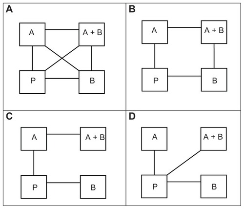
• a full completely connected network

• a “square” network, including the four comparisons P versus A, P versus B, A versus A + B, and B versus A + B

• a “horseshoe” network, including the three comparisons P versus A, P versus B, and A versus A + B

• a “star” network including the three comparisons P versus A, P versus B, and P versus A + B.

These four networks were specifically chosen as they were highly represented in two recent respirology MTCs.^8,9 For all simulations, we simulated five two-arm trials for all included comparisons in the network. We simulated trial sample sizes by sampling the trial sample size with equal probability from all integers between 100 and 500 and between 500 and 1500. The number of patients in each intervention arm was set to half of the trial sample size (rounded up if the trial sample size was an odd number). These sample sizes were based on observations of subtreatment networks of two recent respirology MTCs.^8,9 For all simulations, we assumed an average control group risk of 40%, and sampled the realized trial control group risk from a uniform distribution between 30% and 50%. For all simulations, we assumed a “common” heterogeneity variance on the log OR scale of 0.10 for all comparisons. Again, the chosen parameter values and parameter value ranges were extrapolated from recent respirology MTCs, and were selected to create a “common” yet generalizable set of MTC scenarios.^8,9 In total, we simulated combinations of four different network structures, two different trial sample size distributions, and three different interactions of A and B. Thus, we simulated a total of 24 scenarios.

Models and simulation technicalities

All simulations were run from R. v.2.12.¹⁰ Each MTC data set was simulated (created) from R, and BRUGS was used to analyze each of the simulated data sets with the considered MTC models through WinBUGS.¹¹ For each simulated MTC data set, we used the conventional MTC model (model 1) in which all treatments are assumed to be completely independent, and the additive effects MTC model (model 2) in which treatment effects are assumed to be fully additive. For each scenario, we first simulated five test data sets and checked convergence of all treatment effect parameters and between-trial variance parameters using the Gelman–Rubin convergence diagnostics.¹² Convergence consistently appeared to occur before 10,000 iterations. However, to increase our confidence that convergence had occurred, we decided to use a burn-in of 20,000 iterations. Inferences were subsequently based on 10,000 iterations. For each scenario we simulated 500 data sets.

Analysis of simulated data

For all 24 simulation scenarios we calculated:

• the proportion of estimates of OR_A,P, OR_B,P, OR_A+B,P, and OR_A+B,A that were 20% relatively greater or smaller than the true parameter value. We believe the 20% threshold represents a clinically important overestimate or underestimate

• the coverage of the 95% credible intervals associated with each of the above OR estimates

• the power associated with each of the above OR estimates (we considered 95% credible intervals that did not include an OR of 1.00 as statistical evidence of effect).

Here, the proportion of overestimates and underestimates were our chosen measures of statistical bias, and the coverage and power were our chosen measures of precision. We calculated the above measures under the two considered MTC models, ie, the additive effects MTC model and the conventional MTC model.

Results

Table 2 presents the proportion of overestimates associated with the four comparative OR (OR_A,P, OR_B,P, OR_A+B,P, OR_A+B,A) under the two models. Table 3 presents the proportion of underestimates. Table 4 presents the coverage of the 95% credible intervals associated with the four comparative OR under the two models. Lastly, Table 5 presents the power associated with each of (the statistical tests for) the comparative OR under the two models. Figures 2–5 display, as in the tables, the proportion of overestimates, proportion of underestimates, coverage, and power, respectively. However, the statistics displayed in Figures 2–5 are limited to the simulation scenarios where the trial sample sizes spanned from 500 to 1500.

Figure 2 Proportion of overestimates for comparative intervention effects estimates (OR estimates) of A versus P (OR A), B versus P (OR B), A + B versus P (OR AB), and A + B versus A (OR AB,A) under the two MTC models.

Notes: The black bars indicate the proportion of overestimates under the conventional model (model 1) and the gray under the additive effects model (model 2). The OR parameters are ordered by row, the treatment network type by column, and the degree of additivity/antagonism by row within each sideways bar plot.
Abbreviation: OR, odds ratio.

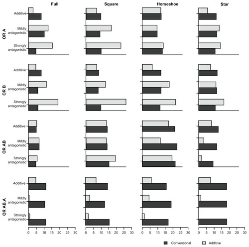
Figure 3 Proportion of underestimates for the comparative intervention effects estimates (OR estimates) of A versus P (OR A), B versus P (OR B), A + B versus P (OR AB), and A + B versus A (OR AB,A) under the two MTC models.

Notes: The black bars indicate the proportion of underestimates under the conventional model (model 1) and the gray under the additive effects model (model 2). The OR parameters are ordered by row, the treatment network type by column, and the degree of additivity/antagonism by row within each sideways bar plot.
Abbreviation: OR, odds ratio.

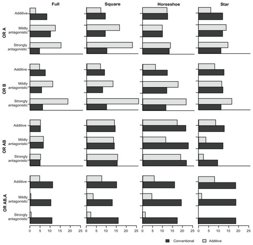
Figure 4 Presents the coverage of the 95% credible intervals associated with the comparative intervention effects estimates (OR estimates) of A versus P (OR A), B versus P (OR B), A + B versus P (OR AB), and A + B versus A (OR AB,A) under the two MTC models.

Notes: The black bars indicate the coverage under the conventional model (model 1) and the gray under the additive effects model (model 2). The OR parameters are ordered by row, treatment network type by column, and degree of additivity/antagonism by row within each sideways bar plot.
Abbreviation: OR, odds ratio.

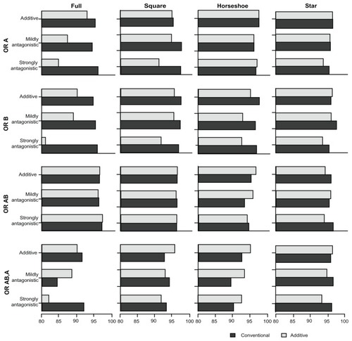
Figure 5 Presents the power with the comparative intervention effects estimates (OR estimates) of A versus P (OR A), B versus P (OR B), A + B versus P (OR AB), and A + B versus A (OR AB,A) under the two MTC models.

Notes: The black bars indicate the power under the conventional model (model 1) and the gray under the additive effects model (model 2). The OR parameters are ordered by row, treatment network type by column, and degree of additivity/antagonism by row within each sideways bar plot.
Abbreviation: OR, odds ratio.

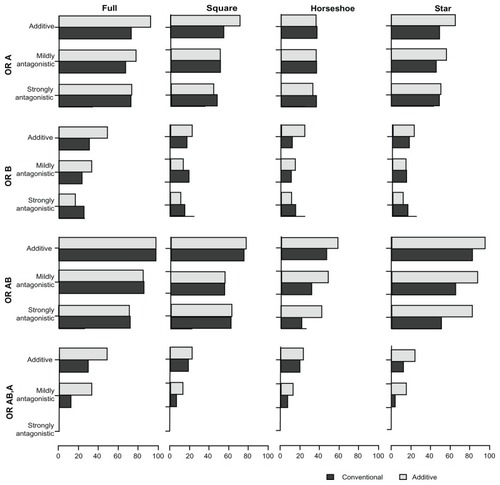
Table 2 Proportion of overestimates for comparative intervention effect estimates (odds ratio estimates) of A versus P (OR_A,P), B versus P (OR_B,P), A + B versus P (OR_A+B,P), and A + B versus A (OR_A+B,A) under the two MTC models

Network type	Trial sample size	Interaction	Proportion of overestimates
			Conventional MTC model (model 1)				Additive MTC model (model 2)
			ORA,P	ORB,P	ORA+B,P	ORA+B,A	ORA,P	ORB,P	ORA+B,P	ORA+B,A
Full	50–500	Strong antagonistic	11.2%	10.8%	9.8%	0.8%	0.4%	0.6%	9.2%	0.6%
Full	50–500	Mild antagonistic	12.2%	10.6%	11.2%	15.0%	4.5%	2.0%	10.8%	16.0%
Full	50–500	Additive	12.2%	12.6%	10.6%	12.6%	5.4%	5.6%	10.8%	5.6%
Full	500–1500	Strong antagonistic	9.0%	5.8%	6.4%	0.2%	0.4%	0.4%	6.4%	0.4%
Full	500–1500	Mild antagonistic	5.6%	7.0%	6.4%	3.6%	0.6%	0.4%	6.6%	0.4%
Full	500–1500	Additive	9.6%	9.4%	8.4%	11.6%	3.0%	5.2%	8.2%	5.2%
Square	50–500	Strong antagonistic	13.6%	15.2%	19.8%	17.8%	3.0%	3.0%	20.0%	28.0%
Square	50–500	Mild antagonistic	15.8%	15.4%	15.4%	14.0%	4.6%	4.8%	15.6%	17.8%
Square	50–500	Additive	18.8%	15.6%	23.0%	17.0%	10.8%	12.4%	22.8%	12.4%
Square	500–1500	Strong antagonistic	10.8%	9.4%	17.4%	15.6%	2.2%	1.8%	17.4%	27.0%
Square	500–1500	Mild antagonistic	9.4%	13.2%	17.4%	14.8%	3.2%	3.2%	17.6%	18.6%
Square	500–1500	Additive	11.0%	9.6%	14.8%	14.8%	8.6%	8.6%	15.0%	8.6%
Horseshoe	50–500	Strong antagonistic	18.0%	18.4%	26.8%	21.8%	18.2%	4.8%	34.6%	28.6%
Horseshoe	50–500	Mild antagonistic	17.8%	14.4%	28.0%	20.8%	18.0%	4.4%	31.4%	18.2%
Horseshoe	50–500	Additive	14.2%	16.8%	26.4%	21.2%	14.8%	11.0%	22.8%	11.0%
Horseshoe	500–1500	Strong antagonistic	11.6%	13.2%	24.2%	20.4%	11.8%	1.4%	34.6%	26.8%
Horseshoe	500–1500	Mild antagonistic	12.0%	10.2%	23.4%	20.2%	12.0%	2.6%	25.6%	24.2%
Horseshoe	500–1500	Additive	12.0%	9.8%	24.2%	20.6%	11.2%	8.2%	17.8%	8.2%
Star	50–500	Strong antagonistic	14.0%	16.4%	12.8%	24.8%	3.4%	5.4%	21.0%	31.2%
Star	50–500	Mild antagonistic	16.2%	17.4%	14.4%	12.4%	8.6%	8.2%	16.4%	8.2%
Star	50–500	Additive	17.4%	17.8%	19.0%	25.0%	12.8%	11.6%	15.6%	11.6%
Star	500–1500	Strong antagonistic	11.2%	12.2%	12.0%	21.0%	1.4%	1.4%	18.2%	33.6%
Star	500–1500	Mild antagonistic	11.4%	9.2%	12.0%	21.2%	4.8%	3.4%	11.6%	19.0%
Star	500–1500	Additive	12.0%	11.4%	11.0%	21.0%	6.4%	7.0%	8.0%	7.0%

Notes: The first three columns indicate which of the 16 simulation scenarios the results on the corresponding row are representative of; columns 4 to 7 present the proportion of overestimates under the conventional MTC model for each of the abovementioned four comparative effects. Columns 8 to 11 present the proportion of overestimates under the fully additive MTC model.

Abbreviations: MTC, multiple treatment comparison; OR, odds ratio.

Table 3 Proportion of underestimates for comparative intervention effect estimates (odds ratio estimates) of A versus P (OR_A,P), B versus P (OR_B,P), A + B versus P (OR_A+B,P), and A + B versus A (OR_A+B,A) under the two MTC models

Network type	Trial sample size	Interaction	Proportion of underestimates
			Conventional MTC model (model 1)				Additive MTC model (model 2)
			ORA,P	ORB,P	ORA+B,P	ORA+B,A	ORA,P	ORB,P	ORA+B,P	ORA+B,A
Full	50–500	Strong antagonistic	8.2%	10.8%	7.6%	12.2%	18.0%	19.4%	8.0%	1.0%
Full	50–500	Mild antagonistic	10.2%	11.2%	8.6%	13.0%	10.4%	13.8%	8.8%	1.6%
Full	50–500	Additive	10.4%	8.0%	8.4%	13.2%	5.6%	4.4%	8.4%	4.4%
Full	500–1500	Strong antagonistic	4.8%	6.2%	5.0%	11.0%	15.4%	18.8%	5.4%	0.8%
Full	500–1500	Mild antagonistic	10.2%	5.8%	6.8%	10.4%	12.6%	11.4%	6.8%	0.6%
Full	500–1500	Additive	8.4%	7.6%	5.2%	11.2%	2.8%	4.8%	5.2%	4.8%
Square	50–500	Strong antagonistic	13.6%	13.6%	18.2%	16.8%	27.0%	26.2%	17.8%	3.0%
Square	50–500	Mild antagonistic	12.4%	13.6%	15.4%	21.0%	16.0%	20.0%	15.2%	5.0%
Square	50–500	Additive	11.0%	13.2%	18.4%	20.8%	11.4%	12.6%	18.6%	12.8%
Square	500–1500	Strong antagonistic	10.2%	10.2%	15.4%	15.6%	23.0%	26.2%	15.6%	1.8%
Square	500–1500	Mild antagonistic	9.4%	8.2%	14.0%	12.6%	16.6%	13.2%	13.6%	2.8%
Square	500–1500	Additive	9.6%	9.0%	14.4%	14.8%	7.2%	7.2%	14.0%	7.2%
Horseshoe	50–500	Strong antagonistic	14.6%	18.8%	22.4%	17.6%	14.6%	25.8%	12.4%	3.2%
Horseshoe	50–500	Mild antagonistic	14.2%	15.0%	22.8%	19.4%	14.2%	19.4%	13.6%	5.4%
Horseshoe	50–500	Additive	14.0%	15.2%	24.4%	19.6%	14.0%	9.8%	20.0%	9.8%
Horseshoe	500–1500	Strong antagonistic	13.6%	11.8%	22.0%	17.4%	13.8%	21.8%	8.6%	1.4%
Horseshoe	500–1500	Mild antagonistic	10.0%	12.2%	22.8%	19.4%	9.8%	17.8%	11.0%	4.6%
Horseshoe	500–1500	Additive	12.4%	12.4%	21.6%	16.0%	12.2%	6.6%	17.4%	6.0%
Star	50–500	Strong antagonistic	16.2%	18.4%	14.4%	22.2%	17.4%	20.6%	6.0%	2.0%
Star	50–500	Mild antagonistic	15.0%	16.2%	17.8%	24.0%	17.6%	17.4%	6.4%	4.6%
Star	50–500	Additive	15.4%	14.2%	15.0%	23.0%	10.6%	10.4%	10.0%	10.4%
Star	500–1500	Strong antagonistic	11.2%	11.2%	9.6%	18.6%	14.6%	16.6%	2.2%	0.0%
Star	500–1500	Mild antagonistic	12.0%	12.2%	12.2%	18.6%	13.6%	11.4%	3.6%	1.6%
Star	500–1500	Additive	12.0%	12.6%	12.8%	18.6%	6.0%	8.0%	8.4%	8.0%

Notes: The first three columns indicate which of the 16 simulation scenarios the results on the corresponding row are representative of; columns 4 to 7 present the proportion of underestimates under the conventional MTC model for each of the above mentioned four comparative effects. Columns 8 to 11 present the proportion of underestimates under the fully additive MTC model.

Abbreviations: MTC, multiple treatment comparison; OR, odds ratio.

Table 4 Coverage of 95% credible intervals for comparative intervention effect estimates (odds ratio estimates) of A versus P (OR_A,P), B versus P (OR_B,P), A + B versus P (OR_A+B,P), and A + B versus A (OR_A+B,A) under the two MTC models

Network type	Trial sample size	Interaction	Coverage of 95% credible intervals
			Conventional MTC model (model 1)				Additive MTC model (model 2)
			ORA,P	ORB,P	ORA+B,P	ORA+B,A	ORA,P	ORB,P	ORA+B,P	ORA+B,A
Full	50–500	Strong antagonistic	95.8%	94.4%	95.6%	91.8%	86.0%	85.2%	96.0%	84.4%
Full	50–500	Mild antagonistic	95.2%	95.8%	97.0%	90.8%	90.6%	89.6%	96.8%	87.8%
Full	50–500	Additive	94.0%	94.0%	95.6%	91.0%	91.6%	94.4%	95.4%	94.4%
Full	500–1500	Strong antagonistic	96.2%	96.0%	97.4%	92.2%	85.0%	81.0%	97.6%	82.2%
Full	500–1500	Mild antagonistic	94.6%	95.6%	96.4%	84.6%	87.4%	88.6%	96.2%	88.6%
Full	500–1500	Additive	95.4%	95.0%	96.6%	91.6%	93.2%	90.2%	96.6%	90.2%
Square	50–500	Strong antagonistic	96.6%	96.0%	94.8%	93.6%	93.0%	92.4%	95.6%	92.4%
Square	50–500	Mild antagonistic	97.0%	98.2%	96.4%	95.8%	95.8%	94.0%	96.4%	95.2%
Square	50–500	Additive	96.8%	95.6%	92.8%	91.6%	94.6%	94.6%	93.2%	94.6%
Square	500–1500	Strong antagonistic	97.6%	97.0%	96.4%	93.4%	91.2%	91.8%	96.4%	91.8%
Square	500–1500	Mild antagonistic	97.6%	97.4%	96.4%	94.2%	94.8%	95.6%	96.2%	93.0%
Square	500–1500	Additive	95.4%	97.6%	96.6%	92.8%	95.0%	95.8%	96.6%	95.8%
Horseshoe	50–500	Strong antagonistic	97.0%	95.4%	94.4%	92.6%	97.6%	90.6%	94.8%	90.6%
Horseshoe	50–500	Mild antagonistic	97.2%	97.4%	96.6%	93.6%	97.0%	94.2%	95.6%	95.4%
Horseshoe	50–500	Additive	96.8%	97.2%	92.2%	92.6%	96.6%	95.4%	95.6%	95.4%
Horseshoe	500–1500	Strong antagonistic	96.8%	97.0%	94.6%	90.2%	97.0%	92.6%	94.2%	92.6%
Horseshoe	500–1500	Mild antagonistic	96.2%	96.6%	93.4%	89.4%	96.2%	93.0%	95.8%	93.4%
Horseshoe	500–1500	Additive	97.6%	97.8%	95.4%	92.6%	97.6%	95.2%	96.6%	95.2%
Star	50–500	Strong antagonistic	95.0%	95.8%	96.4%	95.8%	95.4%	95.2%	95.6%	95.2%
Star	50–500	Mild antagonistic	95.4%	94.2%	95.6%	95.2%	94.8%	94.2%	95.4%	92.0%
Star	50–500	Additive	95.2%	96.0%	94.0%	94.0%	93.6%	95.0%	95.0%	95.0%
Star	500–1500	Strong antagonistic	95.6%	95.4%	96.6%	96.0%	93.6%	93.4%	94.0%	93.4%
Star	500–1500	Mild antagonistic	95.8%	97.6%	95.4%	96.6%	95.6%	96.0%	95.8%	94.8%
Star	500–1500	Additive	96.4%	96.0%	96.0%	95.8%	96.4%	96.4%	94.2%	96.4%

Notes: The first three columns indicate which of the 16 simulation scenarios the results on the corresponding row are representative of; columns 4 to 7 present the coverage under the conventional MTC model for each of the above mentioned four comparative effects. Columns 8 to 11 present the coverage under the fully additive MTC model.

Abbreviations: MTC, multiple treatment comparison; OR, odds ratio.

Table 5 Power associated with comparative intervention effect estimates (odds ratio [OR] estimates) of A versus P (OR_A,P), B versus P (OR_B,P), A + B versus P (OR_A+B,P), and A + B versus A (OR_A+B,A) under the two MTC models

Network type	Trial sample size	Interaction	Power
			Conventional MTC model (model 1)				Additive MTC model (model 2)
			ORA,P	ORB,P	ORA+B,P	ORA+B,A	ORA,P	ORB,P	ORA+B,P	ORA+B,A
Full	50–500	Strong antagonistic	63.4%	25.2%	62.0%	–	66.2%	15.2%	61.4%	–
Full	50–500	Mild antagonistic	59.8%	21.2%	78.4%	11.0%	75.0%	25.2%	78.4%	25.2%
Full	50–500	Additive	62.6%	23.0%	93.4%	25.2%	87.0%	42.0%	93.6%	42.0%
Full	500–1500	Strong antagonistic	73.0%	25.2%	72.6%	–	72.8%	17.0%	71.8%	–
Full	500–1500	Mild antagonistic	66.8%	25.2%	86.2%	12.8%	78.4%	33.0%	85.6%	32.8%
Full	500–1500	Additive	72.2%	28.0%	98.4%	30.2%	92.8%	49.0%	98.4%	49.0%
Square	50–500	Strong antagonistic	38.8%	16.2%	35.4%	–	33.0%	9.8%	33.6%	–
Square	50–500	Mild antagonistic	42.6%	14.6%	41.0%	5.0%	41.0%	9.4%	41.2%	9.4%
Square	50–500	Additive	45.8%	15.4%	65.8%	16.0%	62.6%	20.0%	67.4%	20.0%
Square	500–1500	Strong antagonistic	48.0%	14.8%	40.0%	–	42.8%	10.8%	40.6%	–
Square	500–1500	Mild antagonistic	50.6%	19.4%	55.4%	7.4%	50.6%	14.0%	56.6%	14.0%
Square	500–1500	Additive	53.4%	16.0%	75.4%	18.6%	71.0%	22.8%	77.2%	22.6%
Horseshoe	50–500	Strong antagonistic	31.2%	12.8%	20.4%	–	31.0%	9.8%	34.8%	–
Horseshoe	50–500	Mild antagonistic	31.8%	10.2%	25.0%	7.2%	32.2%	11.6%	41.0%	11.6%
Horseshoe	50–500	Additive	31.8%	11.0%	37.4%	15.4%	33.6%	21.8%	49.8%	21.8%
Horseshoe	500–1500	Strong antagonistic	35.6%	12.6%	21.6%	–	33.8%	10.6%	41.6%	–
Horseshoe	500–1500	Mild antagonistic	36.6%	9.4%	31.2%	8.2%	36.8%	13.8%	48.2%	13.8%
Horseshoe	500–1500	Additive	36.2%	10.2%	46.4%	19.2%	36.0%	24.6%	58.6%	24.6%
Star	50–500	Strong antagonistic	37.8%	13.0%	36.2%	–	37.0%	9.2%	67.2%	–
Star	50–500	Mild antagonistic	34.8%	15.6%	48.4%	3.4%	38.8%	16.2%	74.4%	16.2%
Star	50–500	Additive	39.4%	14.2%	75.0%	8.2%	55.4%	21.4%	89.8%	21.4%
Star	500–1500	Strong antagonistic	48.2%	17.2%	50.6%	–	50.4%	12.2%	82.4%	–
Star	500–1500	Mild antagonistic	45.4%	14.0%	64.8%	3.4%	56.2%	15.2%	87.0%	15.2%
Star	500–1500	Additive	48.8%	17.0%	83.4%	11.8%	65.0%	23.6%	95.2%	23.6%

Notes: The first three columns indicate which of the 16 simulation scenarios the results on the corresponding row are representative of; columns 4 to 7 present the power under the conventional MTC model for each of the abovementioned four comparative effects, and columns 8 to 11 present the power under the fully additive MTC model. No power is reported for OR_A+B,A under simulation scenarios with strong antagonistic interactions because there is no difference between A + B and A in this scenario.

Abbreviations: MTC, multiple treatment comparison; OR, odds ratio.

In the additive scenarios, the proportions of overestimates with the additive model were consistently smaller or similar for all treatment comparisons when compared with the conventional model. In the mildly antagonistic scenarios, the effects of A + B versus A and A + B versus P yielded similar effects under the two models, whereas the effects of the single treatments (A versus P and B versus P) were less frequently overestimated under the additive model. In the strongly antagonistic scenarios, the effects of A + B versus A and A + B versus P were more frequently overestimated under the additive model.

In the additive scenarios, the proportions of underestimates with the additive model were consistently smaller or similar for all treatment comparisons when compared with the conventional model. In particular, the comparison between A + B versus A, and also B versus P, were less frequently underestimated with the additive model. In the antagonistic scenarios (and more pronounced in the strongly antagonistic scenarios), the comparisons A versus P and B versus P were more frequently underestimated with the additive model. However, the comparisons A + B versus P and A + B versus A remained less frequently underestimated with the additive model.

In the additive scenarios, the coverage of the two models was comparable, except for the full network with small sample size trials where the additive model performed slightly worse. Under the mildly antagonistic scenarios, the coverage of the two models was again comparable, except for the full network scenarios where the additive model performed worse. The coverage under the strongly antagonistic scenarios was comparable for the star and horseshoe networks, slightly worse for the additive model for the square network, and considerably worse for the additive model for the full network. However, it should be noted that the coverage for the comparison A + B versus P was similar for the two models in all scenarios.

In the additive scenarios, the additive model yielded considerably greater to similar power for all comparisons when compared with the conventional model. Under the mildly antagonistic scenarios, the additivity model yielded greater to similar power in most cases (the only exception being B versus P in the square network). Under the strongly antagonistic scenarios, the two models were comparable for the full and square networks (although B versus P had slightly lower power under the additive model), but under the horseshoe and star networks, the comparison A + B versus A had considerably more power under the additive model.

Discussion

It is common to provide combinations of individual drugs to patients. Therefore, it is important to assess the effect of a particular combination of drugs relative to that of the individual drugs themselves or to other combinations of interest. Comparative effectiveness can readily be evaluated with MTC, but the conventional modeling approach ignores dependencies between drug combinations (and single drugs) that include the same drug. The additive effects MTC model incorporates this dependency by assuming full additivity of treatment effects, and thereby gains often valuable precision. However, when the additivity assumption is violated, the additive effects model may yield biased effect estimates.

Our simulation study provides insight into the extent to which the additivity assumption may be violated, and the additive effects model will still provide a worthwhile trade-off in precision gain versus model bias. The additive effects model is, not surprisingly, far superior to the conventional MTC model under full additivity. When there exists a mild but potentially important antagonistic interaction, neither of the two models seems better than the other. When there exists a strong interaction, the degree of bias that the additive effects model produces does not seem worth the trade-off in precision gain. Considering the results of the additive and mildly antagonistic scenarios, it stands to reason that the precision-bias trade-off will be in favor of the additive effects model for any scenario where the degree of antagonism lies anywhere between the two scenarios. Thus, it seems reasonable to prefer the additive effects model in situations where the assumption of approximate additivity is sensible.

Our simulation study comes with a number of strengths and limitations. Our simulation parameters were informed by real MTC examples and can thus be assumed applicable to MTCs in chronic obstructive pulmonary disease, and most likely also to similar areas where treatments are used in combination. Being regular readers and authors of systematic reviews, we believe that the spectrum of treatment networks and parameter values chosen for our simulations represent a substantial proportion of published meta-analysis and multiple treatment comparisons. However, our simulations may lack generalizability with respect to the parameters that we did not vary. In this vein, we did not vary the degree of between-trial variation or the control group risk, and we did not vary the combination of treatment effects of A, B, and A + B or the interaction ratio. We limited our simulation to four treatment arms (two active treatments A and B). This design feature is both a strength and a limitation. It is a strength because it facilitates understanding of how the two MTC models work at the basic level and allows for simple interpretation of the results. It is a limitation because most MTCs are performed on larger networks where several drugs may be combined, and potentially, several interactions may occur. We discuss the implications of this in more detail below.

As mentioned above, most MTCs are performed on larger treatment networks. In respirology or other medical areas, this may involve several drug combinations. Typically, only a few of all possible drug combinations will have been compared in head-to-head randomized clinical trials, and perhaps equally infrequent, most individual drugs and drug combinations cannot be compared indirectly. For example, if three active drugs A, B, and C, and all possible combinations thereof, are considered in an MTC, a situation can occur where A + B and A + C have been compared with placebo or any of the individual drugs A, B, and C, but B + C and A + B + C have not. In this situation, the conventional MTC model would not allow for estimation of comparative effectiveness between B + C or A + B + C and any of the other interventions. However, the additive effects of the MTC model would allow for estimation of such comparative effects. We could refer to such estimates as “fully additive estimates”. Whether and when it is sensible to combine evidence in such a manner is discussed elsewhere, and the decision to combine such evidence will typically depend on more than statistical factors. Our simulations demonstrate the statistical soundness of deriving additive effect estimates in the absence of direct comparisons. Checking that other necessary clinical and biological criteria are met will confirm that at least ‘approximate additivity’ holds true.¹³ With this, authors of MTCs can be comfortable in statistically combining direct and indirect evidence with and additive effects MTC model.

In conclusion, the additive MTC model is statistically superior when additivity holds true, and comparably advantageous in terms of its bias-precision trade-off when additivity is mildly violated. This suggests that the additive effects MTC model can readily be used in situations where one can only assert approximate additivity.

Disclosure

This study was funded by Nycomed, Zurich, Switzerland, a Takeda Company and Drug Safety and Effectiveness Network (DSEN), Health Canada.