Causal diagrams and the cross-sectional study

Abstract

The cross-sectional study design is sometimes avoided by researchers or considered an undesired methodology. Possible reasons include incomplete understanding of the research design, fear of bias, and uncertainty about the measure of association. Using causal diagrams and certain premises, we compared a hypothetical cross-sectional study of the effect of a fertility drug on pregnancy with a hypothetical cohort study. A side-by-side analysis showed that both designs call for a tradeoff between information bias and variance and that neither offers immunity to sampling colliding bias (selection bias). Confounding bias does not discriminate between the two designs either. Uncertainty about the order of causation (ambiguous temporality) depends on the nature of the postulated cause and the measurement method. We conclude that a cross-sectional study is not inherently inferior to a cohort study. Rather than devaluing the cross-sectional design, threats of bias should be evaluated in the context of a concrete study, the causal question at hand, and a theoretical causal structure.

Keywords:

• cross-sectional study
• causal diagrams
• colliding bias
• information bias

Of the numerous study designs, the cross-sectional study is often considered an undesired design, perhaps because it is not well understood. The design is often described as a snapshot of a population,¹ an oversimplification; generic claims of bias are common; and the correct measure of association is still debated.² Some of the confusion may be resolved by reevaluating the cross-sectional study using a methodological tool called causal diagrams. Causal diagrams have proved helpful in understanding other research designs^3,4 as well as various sources of bias.⁵

However, causal diagrams are not enough. Any discussion of the merit of some research design should be preceded by difficult questions about causality: how does causality work? What do we want to know about a cause-and-effect relation? Which measure of effect is preferred? Previous writers on the cross-sectional design have set some of these questions aside and argued in favor of one measure of effect or another, but there is no consensus on the matter. For instance, some authors have proposed that the prevalence odds ratio is the preferred measure of effect in cross-sectional studies,² whereas others have discussed the pitfalls of cross-sectional studies assuming that the hazard ratio is the causal parameter of interest.⁶ A discussion of those questions is beyond the scope of this article; instead, we simply present our answers as premises.

We examine the cross-sectional design vis-à-vis the cohort design by using a simple hypothetical example – estimating the effect of a fertility drug on pregnancy. The following premises are proposed: (1) all causation operates between one time point variable and another, later, time point variable. For instance, taking (versus not taking) a fertility drug has a possibly unique effect on pregnancy status at each future time. (2) Effects may be modified by other causal variables.⁷ For example, the effect of a fertility drug may differ according to the level of endogenous estrogen. (3) The preferred measure of effect is the probability ratio (eg, the probability of being pregnant at some future time point after taking a fertility drug divided by the probability of being pregnant after not taking the drug). (4) Causal knowledge amounts to knowing the magnitude of the effect at all future times: the probability ratio a month later, a year later, and at every time point in-between, before, or thereafter. (5) Thought bias aside,⁸ every bias is anchored in some causal structure and can be presented in a causal diagram.

Causal diagrams

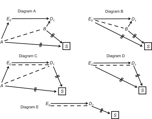
A causal diagram depicts a theoretical causal structure for some set of variables. The variables are displayed along the time axis (left to right) and an arrow connects each cause-and-effect pair (Figure 1). Usually one pair of variables is distinguished as the cause and effect of interest, denoted by E (for “exposure”) and D (for “disease”), respectively – with subscripts that indicate time ordering (eg, E₀, D₁). For example, E₀ may indicate taking, or not taking, a fertility drug at one time, and D₁ may indicate pregnancy status at some later time. If E₀ and D₁ are binary variables, coded 0 and 1, we are interested in the following probability ratios as measures of effect: Pr(D₁ = 1|E₀ = 1)/Pr(D₁ = 1|E₀ = 0) and Pr(D₁ = 0|E₀ = 1)/Pr(D₁ = 0|E₀ = 0). Again, the magnitude of the probability ratios may depend on the time interval between “exposure” and “disease.”

Figure 1 Principles of causal diagrams.

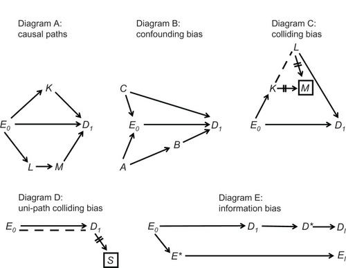
A natural path between E₀ and D₁ is any sequence of arrows, regardless of their direction, that connects the two and does not pass more than once through each variable. A causal path between E₀ and D₁ is any natural path in which all the arrowheads point toward D₁, namely any path through which E₀ affects D₁ (Figure 1, Diagram A). A confounding path is any natural path that contains a shared cause of E₀ and D₁ on that path, such as E ← C → D₁ and E₀ ← A → B → D₁ (Figure 1, Diagram B). The shared cause is called a confounder. Finally, a colliding path is any natural path that contains at least two arrowheads that “collide” at some variable along the path, such as E₀ → K → M ← L → D₁ (Figure 1, Diagram C). The variable at which the arrowheads collide (here, M) is called a collider; its proximal causes on the path are called colliding variables (here, K and L).

Certain theorems establish a mathematical link between a causal diagram and the expected association between any two displayed variables. Specifically, both causal paths and confounding paths contribute to the marginal (“crude”) association between E₀ and D₁, whereas colliding paths do not. For example, in Figure 1, Diagram A, the marginal association between E₀ and D₁ is created by causal paths alone, and therefore the crude probability ratio is an unbiased estimator of the effect of E₀ on D₁. In Diagram B, however, two confounding paths also contribute to the marginal association between E₀ and D₁ (besides the causal path E₀ → D₁), and therefore confounding bias is present. Methods to remove confounding bias are described elsewhere.⁵

Colliding paths are often called blocked paths because they do not contribute to the marginal association between E₀ and D₁ Nonetheless, a colliding path may be “opened” by conditioning on all the colliders along the path. Although conditioning can take numerous forms, the basic form is restricting the collider to one of its values. Such conditioning, denoted by a box, dissociates the collider from all other variables, denoted by two lines over surrounding arrows (Figure 1, Diagram C). At the same time, however, conditioning on a collider may also create or contribute to an association between the colliding variables, denoted by drawing a dashed line (Figure 1, Diagram C). Whether an association is created or altered by conditioning depends on the phenomenon of effect modification. If the colliding variables modify each other’s effect on the collider – and effects are measured by probability ratios – a dashed line should be drawn.

Under these assumptions, new paths may be formed between E₀ and D₁ after conditioning on colliders. Such paths, which may contain only dashed lines or both dashed lines and arrows, are called induced paths because they arise by conditioning on colliders. Conditioning on M induces the path E₀ → K--L → D₁ (Figure 1, Diagram C). This path contributes to the (conditional) association between E₀, and D₁, which no longer reflects the causal path E₀ → D₁ alone. The bias that arises by induced paths is called colliding bias.⁵ As will be seen later, the so-called selection bias⁹ – a central concern in many studies – is a form of colliding bias.

It is best to avoid colliding bias if possible. If not possible, the bias may sometimes be removed by conditioning on some variable along the induced path (which would “reblock” the path). For instance, the path E₀ → K--L → D₁ will be blocked by conditioning on K or L.

A special structure of colliding bias is shown in Figure 1, Diagram D. Here, E₀ and D₁ collide at S, but the causal path from E₀ to S passes only through D₁. To distinguish this structure from classic colliding of separate arrows, it is called uni-path colliding.⁵ Interestingly, it can be shown that uni-path colliding bias does not arise if the odds ratio serves as a measure of effect. We will return to this point in the Discussion.

Lastly, causal diagrams also clarify the meaning of information bias.⁸ The values of E₀ and D₁ are unknown but can be replaced by measured values, which is a causal process, too (Figure 1, Diagram E); the variable of interest affects the measured variable (denoted by an asterisk). It is crucial to understand, however, that every variable is restricted to a distinct time point, and the moment of measurement does not coincide with the moment of analysis. For this reason, the analyzed variables are not synonymous with the measured variables; they are located farther along the causal paths and are denoted by the subscript “I,” short for “imputed” (Figure 1, Diagram E). As their names imply, these variables impute (ie, substitute for) the unknown values of the variables of interest: E_I substitutes for E₀, and D_I substitutes for D₁. We always hope that imputed values are exact copies of the values of interest; however, we can never be certain.

It is easy to explain now the idea of information bias. We wish to estimate the association between E₀ and D₁ (as a measure of effect), but we can only estimate the association between E_I and D_I (Figure 1, Diagram E). If the two associations differ, information bias is present. The bias can be present in every research design, including a randomized trial,¹⁰ and could arise by several causal structures.⁵

Selection and bias

In every study, some variables influence whether someone will take part in the study or not (ie, causes of selection status). These variables may conveniently be divided into four groups: location of the study participant, vital status, selection criteria, and other causes. For example, a study of the effect of a fertility drug on pregnancy might be restricted to certain clinics (location), will obviously recruit women who are alive (vital status), and might enroll women in a specified age range (selection criterion). In addition, participation will likely be affected by other variables, such as perceived benefits and level of interest in research.

That selection is part of any study implies the existence of a binary variable that indicates selection status: selected for the study or not selected. We denote this variable by the letter S and illustrate its causes by the variables A, B, and C (Figure 2). In some designs the exposure itself may be another cause of S – for instance, a study in which women who take a fertility drug are preferentially recruited over those who do not. Notice the position of S on the time axis in a prospective cohort (Figure 2). The variable is located before the time of the effect (t = 1). (To simplify, we depicted S after E₀, but it may be placed before E₀, too.)

Figure 2 A causal diagram for a prospective cohort study (confounders omitted).

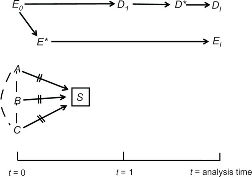
Since only the selected people are eventually studied (S = selected), conditioning on S is inherent in every research design (Figure 2). That is unavoidable but not necessarily harmful as far as colliding bias is concerned. Whether inevitable conditioning on S is a source of bias depends on the postulated causal structure for a given study. In Figure 2, for example, conditioning on S carries no consequences because it is not a collider on any path between E₀ and D₁. In fact, S is not even connected to either variable. As will be seen later, this is not always the case.

Colliding bias may be classified into two types: sampling and analytical.⁵ The former is related to sample selection (conditioning on S) and the latter to analytical decisions with a dataset at hand. We restrict the following discussion to sampling colliding bias because it is relevant to the study design.

Sampling colliding bias in a cohort study

Figure 3, Diagram A shows a structure for a prospective cohort in which E₀ and S share a cause (variable A) as do D₁ and S (variable B). Inevitable conditioning on S (S = selected) induces the path E₀ ← A--B → D₁, and therefore colliding bias is present. For example, in a cohort study of the effect of a fertility drug on pregnancy variable A may be education level (a shared cause of taking a fertility drug and willingness to participate in research) and variable B may be parity status (a cause of future pregnancy status and perhaps a selection criterion). One partial remedy seems obvious: do not select women on the basis of parity status. Parity status, however, might affect participation for reasons other than selection criteria.

Figure 3 Several structures of sampling colliding bias in a cohort study.

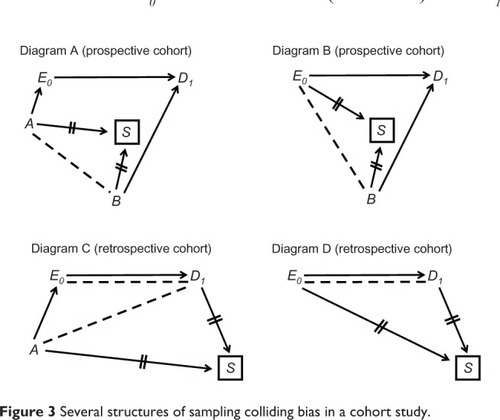
Figure 3, Diagram B shows an example where D₁ and S share a cause as before (variable B) but E₀ is also a cause of S (eg, women who take a fertility drug are more likely to participate in research than women who do not). In this structure, colliding bias is blamed on the induced path E₀--B → D₁. Notice that both Diagram A and Diagram B can exist in a single prospective cohort.

In a retrospective cohort, unlike a prospective cohort, follow-up time is over by the time of selection, which means that S is located after t = 1. It is therefore possible for D₁ to be another cause of S. For example, pregnancy status might affect selection status (perhaps because women who do not become pregnant are more likely to switch clinics than women who do.) The possibility of D₁ → S opens the door to other structures of colliding bias (Figure 3, Diagrams C and D). Notice again that the two diagrams for a retrospective cohort are not mutually exclusive. Moreover, the diagrams for a prospective cohort (Diagrams A and B) could be redrawn to match a retrospective cohort simply by moving S to the right of D₁. In fact, all four diagrams in Figure 3 could be combined into one diagram and might coexist in a single retrospective cohort.

Figure 3 shows only basic examples of sampling colliding bias in a cohort study. Other structures, however, are extensions of the key elements in this figure.

Sampling colliding bias in a cross-sectional study

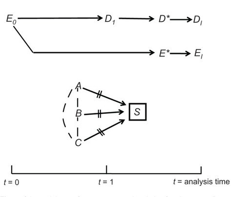
The key feature of a cross-sectional study is the selection of participants at one time past t = 1 (Figure 4). Nonetheless, a comparison of Figure 4 with Figure 2 reveals that the basic causal diagram of a cross-sectional study (Figure 4) is similar to that of a prospective cohort (Figure 2), except that S is located to the right of t = 1 (as in a retrospective cohort). Similarly, inevitable conditioning on S does not have to carry any consequences (Figure 4), which means that colliding bias is not inherent in either design.

Figure 4 A causal diagram for a cross-sectional study (confounders omitted).

Sampling colliding bias in a cross-sectional study could arise by several causal structures (Figure 5), but the similarity to a cohort design is, again, remarkable. The top two diagrams in Figure 5 (cross-sectional study) are identical to the top two diagrams in Figure 3 (prospective cohort), except for the location of S on the time axis. Diagrams C and D in Figure 5 (cross-sectional study) are identical to the respective diagrams in Figure 3 (retrospective cohort). Diagram E in Figure 5 shows uni-path colliding bias, yet that structure can also be found in a retrospective cohort. As before, Figure 5 shows only basic examples of colliding bias in a cross-sectional study. Other structures, however, are extensions of the key elements in this figure.

Figure 5 Several structures of sampling colliding bias in a cross-sectional study.

In summary, some structures of sampling colliding bias in a cross-sectional study can be found in a prospective cohort and every structure can be found in a retrospective cohort. Regardless, scientific inquiry is not founded on the possibility of bias but on proposing an explicit theory for a particular study. A critic of a particular study should propose a structure of colliding bias – with named variables – and allow others to examine and criticize the criticism. It is not helpful to say that selection bias might exist in a cross-sectional study (or in any design) or that one design allows for more structures of bias than another. Generic truism is not part of empirical science.

Information bias in a cohort study

Consider a prospective cohort study of 80 women, the purpose of which is, again, to estimate the effect of a fertility drug on pregnancy. Figure 6 displays the observation time for groups of ten women (solid lines), such that all baseline calendar times are aligned on the X-axis. As shown at the top of the figure, we are interested in estimating the effect on pregnancy status at two time points, t = 1 and t = 2, where Δt = 2 is the maximum follow-up time (subjects 1–20). Dotted lines denote gaps of unobserved times through t = 2 (subjects 21–80). Assume for simplicity that the intervals [t = 0, t = 1] and [t = 0, t = 2] are 1 year and 2 years, respectively.

Figure 6 The tradeoff between information bias and variance in estimating the probability ratio for two effects: E₀ → D₁; E₀ → D₂.

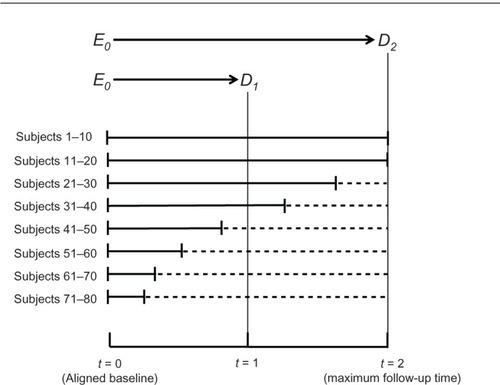
To estimate the effect at two years, E₀ → D₂, we have two extreme options: to rely on data from only 20 women (subjects 1–20) who were observed at t = 2 or to rely on all 80 women and impute the unknown value of D₂ for 60 of them. The imputation is simple; we assume that the value of D (pregnancy status) at the last follow-up time is identical to the value of D₂ (pregnancy status at 2 years). Intermediate options also exist; for example, impute the value of D₂ only for women whose follow-up time exceeds 18 months.

The options above reflect a tradeoff between the size of the variance and the magnitude of information bias. If we rely on only 20 women for whom the value of D₂ is known, no imputation is needed for other women and information bias will be reduced. At the same time, however, the variance will increase because the sample size will shrink from 80 women to 20. Conversely, if we wish to reduce the variance and include all 80 women in the analysis, we must impute the value of D₂ for 60 of them and thereby increase the magnitude of information bias. The same principles hold for estimating the effect of the drug at 1 year, E₀ → D₁ (Figure 6). We can either rely on data from 40 women for whom the value of D₁ is known (subjects 1–40) or impute the value of D₁ for the other 40 (subjects 41–80). Again, intermediate options are possible, too, reflecting different tradeoffs between variance and bias. Unfortunately, no logic can strike a balance between the two; it is our choice.

Figure 7 duplicates the observations in Figure 6 but the X-axis is calendar time. To simplify, we focus on estimating only one effect, E₀ → D₁, and prefer to include all 80 women in the analysis – that is, to minimize the variance at the cost of information bias. The length of the interval of interest (1 year) is depicted in a dotted line above the observed interval (solid line). As can be seen in subjects 41–80, the dotted line is not nested in the solid line, which means that pregnancy status (the value of D at t = 1 year) is not known for these women. Instead, D₁ could be imputed for them from the last available measurement of D (ie, pregnancy status at an earlier time). The nonoverlapping segments of the dotted line indicate the time difference between D₁ and the source of its imputation. In general, the greater the distance between D₁ and the last follow-up, the less accurate the imputation would be and the greater the magnitude of information bias. Notice that in 20 of the above cases (subjects 41–50 and 61–70), D₁ occurs after the end of the study, but we impute its value from a measurement of D that occurred before the date of the last observation.

Figure 7 Estimating the effect E₀ → D₁ by a cohort study (calendar-based graph).

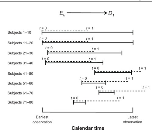
So far it has been simplistically assumed that the value of D is known whenever t = 1 is contained in the window of observation (subjects 1–40). That is not always the case, however, because study participants are usually observed at distinct time points, rather than continuously. For instance, the pregnancy status of a woman might be verified only when she comes to the clinic. In practice, logistical constraints often dictate a need to impute the value of D₁, even when t = 1 is contained within the window of observation. Information bias is always lurking in the background.

Information bias in a cross-sectional study

Figure 8 shows what might have happened if we had tried to study these women in a cross-sectional study. Now t = 1 nearly coincides with the time of the study; the 1-year interval [t = 0, t = 1] is fixed on the calendar; and t = 0 is a historical date, 1 year earlier.

Figure 8 Estimating the effect E₀ → D₁, by a cross-sectional study (calendar-based graph).

At first glance we notice that 30 of the 80 women would not have been selected (subjects 31–40, 51–60, and 71–80) because they were not observed at the time of selection. The consequences for the variance or the bias are far from clear, however. First, other women could have been recruited to reach a sample size of 80. Second, the absence of some observations, by itself, is not a sufficient condition for bias. As we saw earlier, sampling colliding bias depends on a causal structure, and the bias is not unique to a cross-sectional study. In fact, the cohort of 80 women (Figure 7) was not immune to sampling colliding bias, either, because selection is a part of every design.

Far more interesting is the domain of information bias. The key task has changed from imputing the value of D₁ (pregnancy status), as required in a prospective cohort, to imputing the value of E₀ (drug taking) because t = 0 is some arbitrary historical time, 1 year earlier. That is sometimes the biggest challenge of a cross-sectional study. If E₀ denotes the use of a fertility drug on some index date, numerous methods of imputations are possible: (1) obtain the information from a clinic record, relying on a clinic visit that took place as close as possible to the index date. (2) Ask each woman whether she took a fertility drug on the index date. (3) Implement both of the previous methods and develop an imputation algorithm that relies on combined information.

Of course not all methods are equally accurate, but the key point is this. We cannot escape the need to impute the values of variables, neither in a cohort study nor in a cross-sectional study, and there is no universal rule about the quality of an imputation in one design versus another. Information bias, just like colliding bias, should be examined in light of the subject matter of a study.

Ambiguous temporality

Perhaps the most widely known criticism of cross-sectional studies, as compared with cohort studies, is ambiguous temporality: are we estimating the effect of E on D or the effect of D on E? For instance, are we estimating the effect of taking a fertility drug on pregnancy status or vice versa? Nonetheless, the ambiguity arises only if we impute the value of E₀ – drug taking 1 year earlier – from drug taking at the time of the study. No ambiguity arises if we obtain information about drug use at t = 0.

Moreover, as long as we assume that D does not affect E, we may even use a contemporaneous measurement of E to impute the value of E₀. For instance, if the cause of interest were some genotype rather than a fertility drug, hardly anyone would have criticized the use of a current blood sample to impute the genotype 1 year earlier because pregnancy status is not assumed to affect the genotype. Contemporaneous measurements of E and D should not be used only if we assume that D → E, rather than E → D, or that both paths exist (E₀ → D₁, → E₂ → D₃,…). In the first case (D → E), we will mistakenly estimate the effect of D on E instead of the effect of E on D. In the second case (E₀ → D₁ → E₂ → D₃…), neither effect will be estimated without bias.

Discussion

Using certain premises and causal diagrams, we have shown here that a cross-sectional study is not inherently inferior to a prospective or retrospective cohort. All of these designs (and others, too) call for a tradeoff between information bias and variance, and none of them offers immunity to sampling colliding bias. Confounding bias was not discussed because the underlying causal structure – a shared cause of E and D⁵ – does not depend on the study design.

Each type of bias should be evaluated in the context of a concrete study, the causal question at hand and a theoretical causal structure. Generic concerns about what might go wrong in one design versus another do not reveal what has actually happened in a given study. Such considerations often motivate the choice of one design but they are pointless once a study was executed and the data are in. Moreover, it is not enough to argue that bias is present in some study because the magnitude of postulated bias is more important than merely its presence. Small bias, of whatever type, may be negligible and therefore ignored.

It might seem strange that we chose the probability ratio as a measure of effect. Are we interested in estimating the effect of a fertility drug on pregnancy only at several discrete time points, such as t = 1 and t = 2? As explained earlier, we are not. We always want to know the effect at all time points after the exposure E₀. To that end if E* is a measurement of E at some time (denoted t − Δt), then E* may be considered an imputation of E at any time (denoted t − Δt′) – provided we acknowledge the following: the imputation is generally better for nearby times (t − Δt′ ≈ t − Δt) and gets worse the farther t − Δt′ is from t − Δt. Therefore, if D* is a measurement of D at time t, then the association between E* and D* (conditional on the necessary covariates) will estimate the effect of E_{t− Δt′} on D_t for all time intervals Δt′ > 0. However, information bias is usually smaller for intervals Δt′ close to Δt and may be very large for intervals that are much smaller, or much larger, than Δt.

We usually put rough limits on imputation-related assumptions. For instance, if the use of a fertility drug and pregnancy status were determined 1 year apart (Δt = 1 year), we may accept the estimated effect for all time points between 10 months and 14 months (10 months ≤ Δt′ ≤ 14 months), but would likely reject the estimate for Δt′= 24 months. Practically speaking, the probability ratio should be computed for as many times as possible: 1 month, 2 months, 3 months, and so on. The usual constraint is the time points at which E and D were measured and the number of people in whom they were measured. Again, there is no way to avoid the tradeoff between the magnitude of information bias and the size of the variance.

The location of selection status (S) after disease status (D) in a cross-sectional study allows D to be a cause of S. If indeed D → S (and E → D), uni-path colliding bias is present (Figure 5, Diagram E). Two intriguing questions may therefore be asked: should we refrain from selecting participants for a cross-sectional study on the basis of disease status? May we use the design when D affects S for reasons other than selection criteria (eg, the disease affects survival)?

Interestingly, partial answers may be found in case-control studies, where D → S by design: people with the disease (cases) are much more likely to be selected than their disease-free counterparts (controls). The structure E → D → S, with conditioning on S, is built into everycase-control study in which E affects D,³ and the so-called remedy is well known. Analysts of case-control studies compute the odds ratio as a measure of effect rather than the probability ratio because uni-path colliding bias does not arise for odds ratios. The same solution may be proposed for a cross-sectional study, but in both designs the remedy is imperfect. Under the assumption that the probability ratio is the preferred measure of effect, the odds ratio is only useful as an approximation. And if the probability ratio is substantially biased (due to uni-path colliding), the odds ratio is not a good approximation.

A previous attempt to identify conditions for the absence of colliding bias in cross-sectional studies did not rely on causal diagrams but on a theorem that relates associational claims (ie, independence) with bias.⁶ Such a theorem, however, cannot be applied in science. Associational claims, unlike causal claims, can change over time and therefore they cannot be tested in repeated studies. Rather, we must rely on theorems that relate causal claims with bias, and such theorems are necessarily specific to a postulated causal structure.

Conclusion

In summary, a cross-sectional study is not inherently inferior to a cohort study. Rather than devaluing the cross-sectional design, threats of bias should be evaluated in the context of a concrete study, the causal question at hand, and a theoretical causal structure.

Disclosure

The authors do not have any conflict of interest in this work.