A Novel Continuous Sleep State Artificial Neural Network Model Based on Multi-Feature Fusion of Polysomnographic Data

Abstract

Purpose

Sleep structure is crucial in sleep research, characterized by its dynamic nature and temporal progression. Traditional 30-second epochs falter in capturing the intricate subtleties of various micro-sleep states. This paper introduces an innovative artificial neural network model to generate continuous sleep depth value (SDV), utilizing a novel multi-feature fusion approach with EEG data, seamlessly integrating temporal consistency.

Methods

The study involved 50 normal and 100 obstructive sleep apnea–hypopnea syndrome (OSAHS) participants. After segmenting the sleep data into 3-second intervals, a diverse array of 38 feature values were meticulously extracted, including power, spectrum entropy, frequency band duration and so on. The ensemble random forest model calculated the timing fitness value for all the features, from which the top 7 time-correlated features were selected to create detailed sleep sample values ranging from 0 to 1. Subsequently, an artificial neural network (ANN) model was trained to delineate sleep continuity details, unravel concealed patterns, and far surpassed the traditional 5-stage categorization (W, N1, N2, N3, and REM).

Results

The SDV changes from wakeful stage (mean 0.7021, standard deviation 0.2702) to stage N3 (mean 0.0396, standard deviation 0.0969). During the arousal epochs, the SDV increases from the range (0.1 to 0.3) to the range around 0.7, and decreases below 0.3. When in the deep sleep (≤0.1), the probability of arousal of normal individuals is less than 10%, while the average arousal probability of OSA patients is close to 30%.

Conclusion

A sleep continuity model is proposed based on multi-feature fusion, which generates SDV ranging from 0 to 1 (representing deep sleep to wakefulness). It can capture the nuances of the traditional five stages and subtle differences in microstates of sleep, considered as a complement or even an alternative to traditional sleep analysis.

Keywords:

• sleep depth value
• sleep continuity
• EEG features
• timing fitness
• ANN model

Introduction

At present, polysomnography (PSG), which can evaluate the sleep structure of patients, is the most important evaluation method for diagnosing sleep disorders such as narcolepsy and sleep apnea syndrome. PSG involves the simultaneous recording of multiple physiological parameters during sleep, including electroencephalography (EEG) to measure brain activity, electrooculography (EOG) to track eye movements, and electromyography (EMG) to assess muscle tone. Additionally, it monitors respiratory effort and airflow, heart rate, and oxygen saturation levels to detect any disruptions in breathing. These signals are crucial for identifying the specific characteristics of sleep disorders and for determining the most appropriate treatment strategies. Following the Rechtschaffen and Kales rules (R&K rules), the state of PSG data (30 seconds as a period) is described as one of the five sleep stages,¹ which are wake (w), non-rapid eye movement period (N1, N2, N3) and rapid eye movement period (REM). However, in practice, as an insufficient description of sleep processes, also affected by subjective or objective conditions, the main drawback of R&K rules is that the results can lead to a lack of consistency.² Although the sleep process can be described as one of the five sleep stages, the low temporal resolution and insufficient number of stages actually destroys the continuity of the sleep process, resulting in a rough sleep structure, which cannot reflect the sleep details when analyzing the data of sleep disorders. In recent years, the analysis of polysomnography data mostly focuses on the study of automatic sleep staging as opposed to manual methods, aiming to facilitate rapid and precise automated classification. Essentially, there are two primary approaches: the conventional machine learning method, which relies on statistical features, and the deep learning approach, grounded in various neural network architectures.

In the conventional approach, the foundation of automatic sleep staging lies in the extraction of sleep features and the application of diverse classification algorithms, including support vector machines, random forests, and others.^3–5 The researchers selected features ranging from the time domain, frequency domain, to nonlinear characteristics for automatic sleep staging.⁶ Multiscale entropy, which exhibited significant differences across distinct sleep stages, was selected as a key feature.⁷ In the frequency domain, the power spectrum and power ratio of different frequency feature waves obtained through wavelet transform were excellent features.⁸ In nonlinear features, it was found that measures such as correlation dimension, Lyapunov exponents, approximate entropy, and detrended fluctuation analysis were typical features.⁹ In the choice of classifier models, some opted for Random Forest,¹⁰ while others used Linear Discriminant Analysis (LDA),¹¹ with accuracy rates around 80% to 90%. The research above clearly shows that the cornerstone of research in automatic sleep staging lies in the analysis of characteristics derived from sleep data.

Compared with the traditional approach, the deep learning methods of staging do not require strict feature extraction but highly affected by the design of neural network structure and the computing ability of the computer.^12–14 It could achieve an accuracy rate of 84.5% using neural networks.¹⁵ The researchers employed Multilayer Perceptron (MLP) neural networks for automatic sleep staging,¹⁶ reaching an accuracy rate of 74.7%. A one-dimensional convolutional network for sleep staging was proposed,¹⁷ achieving an accuracy rate of 87%. Recurrent Neural Networks (RNNs) for sleep staging could reach accuracy rate of 87.2%.¹⁸ A new network for sleep staging called Deepsleepnet,¹⁹ which utilized two convolutional neural networks to extract time-frequency features from EEG data, combined with Long Short-Term Memory (LSTM) networks to extract associations between different sleep stages, reached an accuracy rate of 82.0%. Some researchers developed a deep learning model based on images for automatic sleep staging, using Class Activation Maps to visualize key reasoning areas,²⁰ with an accuracy rate exceeding 80%, while others employed a multimodal architecture with residual units to address the vanishing problem in deep learning,²¹ achieving a classification accuracy rate of 87.34% and an F1-score of 87.42%. For sleep staging based on deep learning, the requirements for feature extraction are not high; however, overall, the staging accuracy results do not significantly outperform machine learning algorithms based on feature selection.

Given the continuous and intricate nature of the sleep process, some researchers pointed out that relying solely on 30-second epochs to categorize it into five distinct stages could pose certain challenges in achieving accurate sleep staging.²² For instance, a 30-second interval classified as wakefulness might encompass brief sleep episodes of less than 15 seconds. Once the threshold of 15 seconds is surpassed, the stage is then categorized as sleep. Conversely, in intervals designated as sleep, it was specified that any periods of wakefulness lasting less than 15 seconds were overlooked.²³ Additionally, the background EEG activity within the same sleep stage can exhibit significant visual differences across various periods and among different patients. Some researchers mentioned that aside from sporadic spindles or K-complexes, the EEG activity in N2 may closely resemble that of N1.²⁴

Currently, these studies aim to investigate the fundamental mechanisms of sleep; however, the clinical significance of these gradual changes in the EEG remains unclear. Therefore, a measure of sleep continuity is highly beneficial for examining the intricate sleep process. For instance, patients with equivalent N2 sleep durations may exhibit substantial differences in their average sleep depth as revealed through continuity measure analysis. At present, few researchers employ continuous quantities to characterize the sleep/wake state. An EEG analysis technique has been introduced that employs a 10th-order autoregressive (AR) model to fit the EEG signal on a second-by-second basis using the Burg algorithm, which estimates AR model coefficients through the least squares method. The resulting 10 AR coefficients constitute the feature vector, which is then utilized to train a multilayer perceptron (MLP) model. The model’s output is a three-dimensional vector that represents the probabilities associated with wakefulness, REM sleep, and deep sleep.²⁵ However, the paper in question did not address the suitability of the 10 AR coefficients as features and did not consolidate the three probabilities into a unified sleep probability value, which could more accurately reflect the cohesive nature of the sleep process. In a separate study, the primary objective was to detect and quantify sleep arousals by measuring or quantifying sleep depth. This was achieved predominantly through autoregressive (AR) power spectral density (PSD) estimation to obtain the time-frequency map of the EEG signal during sleep arousals. The classification performance of potential standard signals was evaluated under various criteria using ROC curve analysis. The findings suggested that the sum of the absolute powers in the alpha and beta bands, as indicated by AUC analysis, served as a reliable continuous marker for sleep depth.²⁶ Nevertheless, this paper did not examine multiple features during the sleep process, and the AR PSD, while a valid feature extraction method, was not the sole approach. The paper acknowledges that sleep arousal is a complex phenomenon that may not be entirely defined by changes in the EEG signal’s spectral characteristics. Although ROC and AUC, based on statistical methods, can serve as markers for sleep depth, they do not inherently form a continuous model from sample data values but rather offer a data-driven analytical approach. Additionally, some researchers have developed a ratio-based index termed the odds ratio product (ORP), designed to assess the likelihood of wakefulness based on the power values of four distinct waveforms: delta, theta, alpha, and beta. This method segments the statistical samples of these four features into 10 intervals, creating 10,000 unique combinations, each with a distinct ID. Consequently, every 3-second EEG segment is assigned a specific ID, and the ratio of wakefulness to sleepiness under that ID is computed and scaled to a range between 0 and 2.5, thereby reflecting the continuous state of sleep.²⁷ While this approach allows for a more refined categorization of sleep states compared to the traditional 5-category sleep staging, it essentially provides a discrete empirical statistical samples value rather than a true continuous measure. Furthermore, the paper does not justify the choice of the four waveform power spectrum features, resulting in a shortfall in the analysis of the selected features.

Among the various methods for collecting, organizing, and studying continuous representations of sleep process, many researchers have conducted more in-depth studies building on the foundation of ORP method. The product ratio method was employed to compute results as a basis for interpreting studies using novel sleep EEG biomarkers, aiding in the differentiation between insomnia and OSA.²⁸ Meanwhile, it also applied to obtain information on sleep disorders that traditional indicators could not capture.²⁹ The sleep structure types were generated to identify patients adversely affected by OSA and predicted patients whose sleep would improve with CPAP treatment.³⁰ At the same time, it was employed in sleep scoring to accurately estimate the scorer’s ability in sleep staging, and reduce inter-rater disagreement.³¹ The product ratio method was also utilized to appraise the intervention-related alterations in non-REM sleep depth.³² Some researchers employed the product ratio method and discovered a novel association between sleep depth EEG biomarkers and adolescent sleep apnea.³³ It was used to identify the correlation between slow wave activity in children and adolescents and the internalization of product ratio indicators.³⁴ However, all the research above has been customary to employ waveform power values as variables in the computation of a continuous index used for evaluating sleep depth. Nevertheless, compared to many other sleep characteristics, whether the timing fitness of power value features is most appropriate for the sleep depth index remains an area that requires more comprehensive investigation.

In this paper, we first generate the sample values of continuous sleep depth based on the fusion of multiple features, which is an empirical value that makes no a priori assumptions about what constitutes awake or sleeping EEG patterns. Next, we train artificial neural networks using this measure samples to produce a Sleep Depth Value (SDV) and evaluate its effectiveness. The paper demonstrates that (a) the SDV accurately predicts when a patient is awake, asleep, or in an ambiguous state; (b) from the statistical samples, it is evident from the awake to N1 and N3 stages, both the mean and standard deviation of the sleep sample values and SDV progressively decrease; (c) in the same R&K stage, the scale of SDV is highly variable within and between epochs and patients; and (d) the pattern of change in the SDV aligns with the occurrence of arousals, making it useful for their detection.

Methods

Data Processing Procedure

The datasets were provided by the Department of Respiratory Sciences of Binzhou Medical College, including 50 groups of normal and 100 groups of obstructive sleep apnea–hypopnea syndrome (OSAHS), which were collected and generated by the Computerics E multi-channel sleep instrument. The total duration was around 1400 hours, including 3 EEG pathways, 2 EOG pathways, 1 EMG pathway, and other pathway signals such as electrocardiogram (ECG) and blood oxygen saturation detection. Signals were captured at a sampling rate of 256 Hz. An accomplished polysomnographic (PSG) technologist reevaluated the recordings, meticulously scoring each 30-second interval for sleep stages, arousals, and respiratory activities in compliance with the American Academy of Sleep Medicine’s standards.

The algorithm was developed by Matlab R2018b with machine learning toolbox. The computer used for processing contained CPU i7-8700, 32G RAM, 2T HDD and so on. Figure 1 presents the flow diagram, which is composed of three distinct parts:

Figure 1 (A–C) Flow chart of the algorithm.

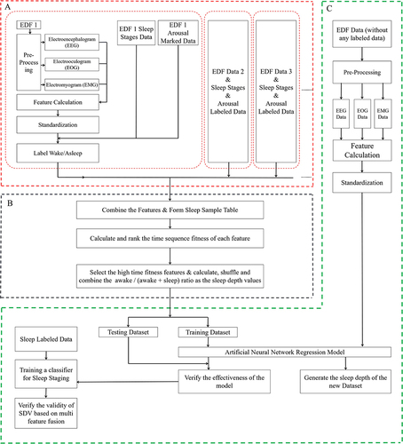
In part A, the pre-processing of EDF data, which includes the manual labeling of sleep stages and arousal information, is completed. This part encompasses feature extraction, standardization, and the computation of the Wake/Asleep ratio;

In part B, calculating and ranking the features by the time sequence fitness firstly; Then calculating, shuffling and combining the awake/(awake + sleep) ratio as the sleep depth sample values based on the features with high timing fitness scores;

In part C, based on all annotated data, we derive a comprehensive training candidate data set through multi-feature fusion and subsequently construct and evaluate an Artificial Neural Network model, which is capable of estimating the sleep depth value (SDV) for any PSG record independent of manual sleep staging and arousal labeling. The model’s efficacy is systematically validated.

Multi-Feature Selection

For the EEG signal, given its weak nature and the presence of substantial background noise, it is easy to be interfered from sources such as facial muscle and eye movement activities. As a non-stationary stochastic signal, feature extraction poses a significant challenge. Consequently, following the AASM-recommended filtering criteria for each channel (bandwidth standard of the EEG signal band-pass filter set between 0.3 and 35Hz), a Butterworth filter with a passband frequency of 0.3 to 35Hz has been implemented for filtration purposes.

In this paper, we selected a total of 38 time and frequency features, which are as follows, numbered from F1 to F38, in which F1 is average energy in the frequency domain, F2 to F5 are relative energy of alpha, beta, theta, and delta waves, F6 to F9 are absolute energy of alpha, beta, theta, and delta waves, F10 to F16 are ratios of band energies: delta/alpha, delta/beta, delta/theta, theta/alpha, theta/beta, alpha/beta, (delta + theta)/(alpha + beta), F17 to F21 are mean, root mean square, variance, skewness and kurtosis, F22 to F25 are duration of alpha, beta, theta, and delta bands (Short-time Fourier transform threshold settings: delta = 50μV, theta = 25μV, alpha = 25μV, beta = 25μV), F26 is spectral entropy, F27 to F30 are local mean difference values of alpha, beta, theta, and delta waves, F31 to F34 are local entropy of alpha, beta, theta, and delta waves, F35 to F38 are maximum amplitude values of alpha, beta, theta, and delta bands.

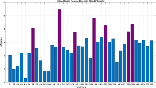
In this study, we employed a random forest model with all 38 features to evaluate the temporal consistency between input features and manually annotated sleep stages. The model’s construction process, which involves the random selection of features from multiple decision trees, places significant emphasis on the number of segmentation points a feature can provide as a key measure of its classification accuracy. A higher number of segmentation points indicate greater significance for the feature. Throughout the training process, we meticulously documented various metrics, including the total number of feature splits and total information gain, with an average calculated over multiple iterations to quantify the temporal consistency of the features. Notably, Features 6 through 9, representing the power value characteristics of alpha, beta, theta, and delta waves, exhibited pronounced temporal characteristics, with the beta wave feature being particularly notable for its high timing fitness. After thorough analysis and scoring, we identified Feature 7 (Absolute energy of beta waves), Feature 14 (The ratio of energy bands for theta to beta), Feature 18 (Root mean square of the signal), Feature 23 (Duration of the beta band with a short-time Fourier transform threshold setting of 25μV), Feature 26 (Spectral entropy), Feature 32 (Local entropy of beta), and Feature 33 (Local entropy of theta) as having a high temporal fit, making them particularly relevant for the temporal consistency analysis of sleep stages. These findings are illustrated in Figure 2, which provides an analytical chart focusing on the temporal consistency of the 38 features, highlighting the estimations of these specific features.

Figure 2 Multi-feature selection based on timing fitness.

Calculation of SDV Sample Values

First, during data processing, each 3-second period is marked as wakefulness or sleep; specifically, phase W and the period contain arousal are categorized as wakefulness, while all other stages are considered sleep; second, to analyze sleep data with multiple features, we begin with selecting the basic waveform energy value feature as the foundation for statistical distribution, which are divided into 10 equal sample intervals, and formed a variety of energy combination values for the four fundamental waveforms: alpha, beta, theta, and delta; third, for each waveform power combination value, we count the number of occurrences corresponding to wakefulness and sleep, and then calculate the ratio of wakefulness to the sum of sleep and wakefulness, which serves as the baseline value for sleep depth; Fourth, after building on this baseline value, the temporal consistency of multiple features is considered and the top N features (in this case, temporarily set at 7) are selected to compute a ranked combination based on the characteristic values of these N features. Each combination will comprise several baseline sleep depth values; fifth, to obtain a representative SDV sample value after feature fusion for an N-feature combination, we weigh each feature by its temporal consistency degree and calculate the weighted average. This approach ensures that features with higher temporal consistency contribute more significantly to the final sleep depth estimation.

Table 1 is the statistical result of the SDV sample values of all the data, including the average numbers of 3-second period, percentages of total, the mean and standard deviation of SDV sample values in each sleep stages. In Table 1, as sleep stages change from Awake to N3, the mean value of the SDV samples decreases from 0.7 to 0.03, and the variance drops from approximately 0.27 to around 0.09. This indicates that the closer to the awake state, the greater the fluctuation in sleep depth, whereas proximity to deep sleep is associated with less variability. Moreover, during the REM stage, both the mean and variance of the Sleep Depth Value (SDV) samples increase in comparison to those in the N3 stage, indicating that arousals contribute to fluctuations in the sleep process, which aligns with observations from real-world sleep patterns.

Table 1 Statistical Results of the Sleep Depth Sample Values

Sleep Stages	Mean of # 3s Epochs/Patient	Std of # 3s Epochs/Patient	Percentage in Total (%)	Mean of SDV	Std of SDV
Awake	2397	1645	24.87	0.7021	0.2702
N1	803	672	8.33	0.2353	0.2709
N2	3380	1067	35.07	0.1202	0.1907
N3	1664	486	17.27	0.0396	0.0969
REM	1393	567	14.46	0.1847	0.2043

Notes: Results expressed as arithmetic mean and standard deviations. “Mean and Std of # 3s epochs/patient” and “Percentage in Total” are calculated based on the manual labeled data. “Mean and Std of SDV” are calculated based on sleep depth sample values.

Abbreviations: # 3s epochs/patient, Number of 3s epochs per patient; SDV, Sleep Depth Value; Std, Standard Deviation.

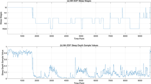
Table 1 shows the statistical results of sleep depth sample values. However, for different EEG data sets, the results will differ. Figure 3 is the sequence diagram of SDV sample values after multi-feature fusion finally generated from specific EEG data. In Figure 3, (a) is the manually calibrated sleep staging map, and (b) is the generated SDV sample value map for every 3 seconds. It can be seen from the above figure that the sample value of sleep depth calculated according to 3 seconds can basically reflect the continuity of the sleep process. From phase W to phase N3, it is a continuously changing process. In phase N3 and phase N2, it can be seen that the sleep depth values are convex, which can reflect the change of sleep depth during sleep. Even in the same sleep period, the sleep depth values are different. If we only consider the sleep stages, we cannot see the changes in sleep during a certain sleep period.

Figure 3 Comparison between sleep depth samples and sleep stages. (a) is the manually calibrated sleep staging map, with the horizontal axis representing time points (a point every 3 seconds), and the vertical axis representing sleep stages; (b) is the SDV sample values map for every 3 seconds.

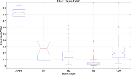
From a statistical perspective, we combine the manually marked sleep staging results and sleep depth sample values after multi-feature fusion. The distribution of sample values in different sleep stages is counted, and the results are shown in Figure 4. The x-axis is mapped to the various sleep stages, namely Wake (W), N1, N2, N3, and REM, whereas the y-axis depicts the corresponding values for sleep depth, scaled from 0 to 1. Within this spectrum, a value of 0 signifies the deepest sleep, and a value of 1 denotes the state of complete wakefulness. It can be seen from the figure that the distribution range of sample values of sleep depth in phase W is 0.7–1, with an average above 0.8, 0.1–0.4 in phase N1, with an average of about 0.3, 0–0.2 in phase N2, with an average of about 0.12, 0–0.08 in phase N3, with an average of under 0.05, 0.15–0.3 in phase REM, with an average of about 0.2. The statistical results from a single data set differ from those of multiple data sets in Table 1 particularly in terms of mean and variance. It is also evident that there are some outliers in different sleep stages, which are directly related to the individuals being tested. Therefore, it is necessary to establish an accurate SDV prediction model based on the statistical sleep depth samples.

Figure 4 Statistical result of sleep depth samples.

Development of the ANN Model

From the above discussion, it is evident that statistical sample values of sleep depth are generated based on feature values with strong time correlation. The relationship between the results under multiple feature fusion and the features themselves is very complex and not linear. Therefore, establishing a joint distribution model for multiple random variables from a mathematical perspective is extremely challenging. In this paper, we opt to construct and train an artificial neural network model to predict sleep depth values (SDV).

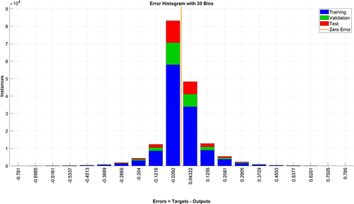
Utilizing the SDV sample values, a selection of multiple features with high temporal coherence is treated as random variables. An Artificial Neural Network (ANN) is constructed, where the feature values serve as inputs and the corresponding SDV samples serve as outputs for model training. The architecture comprises seven neurons in the input layer, corresponding to the chosen features, two hidden layers each with six neurons, and an output layer with a single neuron representing the SDV value ranging from 0 to 1. The training parameters are set with a maximum iteration count of 1000, a target error of 10⁻⁵, a learning rate of 0.01, and a momentum coefficient of 0.9. As depicted in Figure 5, the error distribution for training data, validation data, and test data is confined between −0.0392 and 0.0432, suggesting the efficacy of the proposed model.

Figure 5 Error histogram of ANN model.

Results

The result of sleep depth values (SDV) based on multi-feature fusion from the ANN model is validated mainly in the following three aspects:

Verification of ANN Model

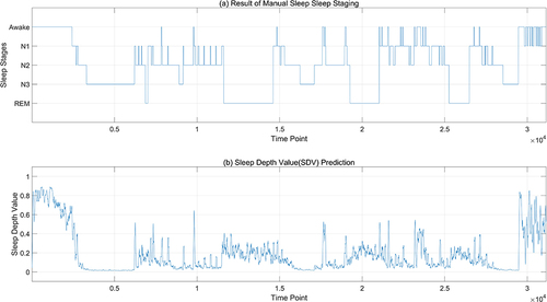
Figure 6 illustrates a comparison between the sleep depth values predicted by the ANN model and those that are manually staged. The figure reveals that the predictions generated by the sleep depth model more accurately reflect the changes in sleep continuity compared to the manually labeled data. Notably, even within stable sleep stages, there are fluctuations in the predicted sleep depth values, aligning with the natural fluctuations observed in the sleep process.

Figure 6 Prediction result of ANN model. (a) is the manually calibrated sleep staging map, with the horizontal axis representing time points (a point every 1 seconds), and the vertical axis representing sleep stages; (b) is the sleep depth values predicted by the ANN model.

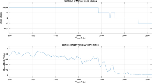
Figure 7 enlarges the details of the part between 500 and 3500 seconds in Figure 6. The progression of the overall sleep process is clearly delineated, transitioning from Awake through N1 and N2 stages, ultimately reaching deep N3 sleep as depicted by the sleep depth values. Initially, during the Awake stage, the SDV (Sleep Depth Value) gradually descends from approximately 0.8 to around 0.6. Between 2000 and 2500 seconds, despite the SDV momentarily dipping below 0.6, it experiences an upward trend, while the sleep stage remains labeled as Awake. This suggests that even within the wakeful state, there are varying intensities of sleepiness. At around 2500 seconds, a sharp decline in SDV signifies the onset of N1 sleep. However, the subsequent rise in SDV between 2500 and 2600 seconds does not surpass 0.45, indicating a stabilization within the N1 phase. Around 2600 seconds, the SDV plunges further to 0.2, indicative of entry into the N2 stage, yet at roughly 2700 seconds, it ascends to 0.4, causing a temporary reversion from N2 back to N1. Following this fluctuation, the SDV swiftly decreases and stabilizes beneath 0.1, transitioning from N1 back to N2 before advancing into N3 sleep. This analysis reveals that the model’s predictions concerning sleep depth values offer a more nuanced perspective of sleep compared to conventional sleep staging, uncovering significant variances in sleep depth even within identical stages.

Figure 7 Details of prediction result. (a) is the details between 500–3500 seconds of manually sleep staging result; (b) is the details between 500–3500 seconds of sleep depth values predicted by the ANN model.

Verification Based on Machine Learning

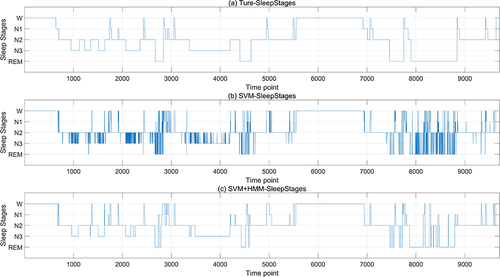
The SDV outcomes derived from the ANN model based on the multi-feature fusion serve as the input layer, while the manually labeled sleep stage data constitute the output layer. The machine learning algorithm is trained using a 10-fold cross-validation approach (with 90% allocated for training and 10% for testing) to validate its efficacy. Given that the classification labels are W, N1, N2, N3, and REM, and there is a considerable disparity in the quantity of data across different classes, leading to an imbalance, the enhanced MSMOTE algorithm is employed for oversampling to create a balanced dataset for model training. Then, this paper initially applies KNN, Random Forest and SVM classifier to classify the data segmented into 3-second intervals, followed by a refinement of the results using the Hidden Markov Model (HMM). It is found that these three classification models derived from three-second intervals exhibit numerous burrs. This is attributable to the brevity of the three-second epochs. One 30-second epoch can be labeled with one sleep stage, while the ten 3-second periods it contains may have different sleep stages. These three classification models also fail to encapsulate the transitional relationships between consecutive time periods. Therefore, for comparison with the manual sleep staging based on 30-second epochs, this paper aggregated every ten 3-second outcomes to produce a 30-second staging result. Then, the sleep staging results are processed using the Hidden Markov Model (HMM), which is capable of handling data with time-series characteristics. The HMM takes the sleep states (Awake, N1, N2, N3, and REM) and the observed data (polysomnograms) as training data, learning the transition patterns between different sleep states and the distribution of the observed data under each state, ensuring that the results align with the temporal sequence properties of sleep staging. The results of the validation process are depicted in Figure 8, with the SVM model serving as an illustrative example. The first diagram represents the manually annotated sleep stage, the second displays the SVM-classified stages based on three-second epochs, and the third presents the outcome following HMM refinement of the SVM results.

Figure 8 Sleep staging result based on SDV. (a) is the manually calibrated sleep staging map, with the horizontal axis representing time points (a point every 3 seconds), and the vertical axis representing sleep stages; (b) is the SVM-classified stages result based on 3-second epochs; (c) is the result of SVM refined by HMM model.

In Table 2, the average accuracy and standard deviation of the classification results for different sleep stages by different algorithms are, respectively, summarized, along with the overall average accuracy and overall standard deviation. From the perspective of different sleep stages, the accuracy rate for the Awake stage is high overall, and slightly improves after HMM correction; the determination of the N1 stage has the lowest accuracy rate, which significantly improves after HMM correction but is still the lowest compared to other stages, not exceeding 50%. However, since the N1 stage does not occupy a high proportion of the sleep process, its impact on the final accuracy is not significant; the mean and std of accuracy results of N2 are both higher than N3 stages; the REM stage is distinguished with the aid of eye movement signals, and the accuracy rate can reach 89% after HMM correction. It can be seen from Table 2 that using only KNN, Random Forest, and SVM algorithms, the total accuracy rate does not exceed 81%, and the accuracy can be improved by about 10% after correction with the HMM algorithm; on the whole, the accuracy rate is highest after correction with the SVM combined with the HMM algorithm, reaching 90.07%. This indicates that due to the characteristic of SDV values that can reflect the details of the sleep process, simple classification algorithms can achieve effective automatic sleep staging.

Table 2 Accuracy Results of Sleep Stage Classification

Sleep Stages Algorithm	Awake Accuracy	N1 Accuracy	N2 Accuracy	N3 Accuracy	REM Accuracy	Total Accuracy
KNN (mean)	85.66%	17.10%	70.44%	63.02%	60.11%	67.01%
KNN (std)	0.0751	0.1031	0.136	0.2231	0.1596	0.0614
Random Forest (mean)	91.02%	25.09%	76.87%	63.69%	62.97%	71.79%
Random Forest (std)	0.0811	0.0732	0.106	0.2091	0.1329	0.057
SVM (mean)	95.63%	20.30%	87.82%	78.74%	73.29%	80.47%
SVM (std)	0.0751	0.0908	0.1302	0.236	0.1825	0.0696
KNN+HMM (mean)	90.30%	34.06%	78.69%	79.19%	78.12%	77.87%
KNN+HMM (std)	0.0795	0.2017	0.1866	0.2542	0.1912	0.0822
Random Forest+HMM (mean)	91.16%	40.47%	85.50%	79.07%	82.07%	81.55%
Random Forest+HMM (std)	0.0892	0.2433	0.1682	0.2588	0.1772	0.0925
SVM+HMM (mean)	98.12%	39.01%	95.26%	93.33%	89.12%	90.07%
SVM+HMM (std)	0.076	0.158	0.1793	0.2558	0.2008	0.0805

Notes: Results expressed as accuracy between the ground truth and the sleep stages prediction generated by K-Nearest Neighbors, Random Forest, and Support Vector Machine. The Hidden Markov Model method is used to improve the result from these three algorithms.

Abbreviations: KNN, K-Nearest Neighbors; SVM, Support Vector Machine; HMM, Hidden Markov Model.

Verification Based on the Arousal Recognition

During N1, N2, N3, or REM sleep stages, if there is a sudden alteration in EEG frequency—including alpha, theta, or any EEG wave with a frequency exceeding 16Hz (excluding spindle waves) with a duration surpassing 3 seconds, and this shift occurs after at least 10 seconds of stable sleep, it can be manually identified as an arousal. If it happens during the REM phase, there should also be a concomitant increase in the amplitude of submental electromyography that persists for no less than 1 second. In this paper, the sleep depth values of several sets of data at the artificially marked arousal points are computed. The arousal segment encompasses the 3-second period of the arousal duration itself, along with the initial 12 seconds and the final 3 seconds, totaling 18 seconds in duration.

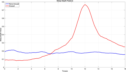
First of all, the alteration in sleep depth at the point of arousal should conform to a pattern that progresses from the lower SDV of sleep states, to the elevated values indicative of an arousal state, and subsequently back to the reduced values associated with sleep states. In this paper, 100 instances of manually marked arousal signals are randomly chosen for comparison with 100 signals captured during non-wake periods in N1, N2, N3, and REM phases to contrast the varying patterns of SDV changes. This comparative analysis is depicted in Figure 9. The pattern of sleep depth value changes during arousal generally aligns with the anticipated judgment criteria. The mean value of the sleep depth during arousal can exceed 0.7, and there is a gradual increase in sleep depth values from 0.1 to 0.3 within the 10 seconds preceding an arousal, which is a continuous process of change and increment that reflects the described continuity of sleep depth variation. Post-awakening, the sleep depth values progressively descend below 0.3, with the period of sleep depth values remaining above 0.3 lasting approximately 6 seconds.

Figure 9 Statistical result of SDV in arousal period.

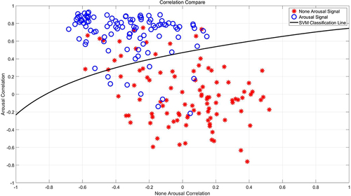
Secondly, 100 arousal signals and 100 non-arousal sleep signals, each with a duration of 18 seconds, are randomly chosen. The respective average sleep depth values from the previously mentioned segment (illustrated in Figure 9) are utilized as benchmark templates for wakefulness and non-wakefulness states, respectively. Simultaneously, an additional randomized selection is executed without replacement from the available data to compile a validation dataset composed of 100 arousal signals and 100 non-arousal sleep signals. Then, the correlation between each 18-second signal in the validation dataset and the sleep depth value templates for wakefulness and non-wakefulness is calculated by utilizing the Pearson correlation coefficient as a measure of similarity. This coefficient is scaled from −1 to 1, where −1 denotes a negative correlation, 1 signifies a positive correlation, and 0 represents an absence of correlation. Subsequently, an SVM classification model is then trained using these signal sleep depth values in a 5-fold cross-validation scheme to verify the accuracy in discerning whether signals indicate arousal. The detailed results are exhibited in Figure 10, which illustrates the correlation between signals and non-wakefulness templates on the abscissa, contrasted with the ordinate showing the correlation between signals and wakefulness templates. The blue circles denote the 100 arousal signals, while the red dots represent the 100 non-arousal signals. The delineation is provided by the classification line derived from the support vector machine employing a Gaussian kernel. Employing a 5-fold cross-validation method yields an average accuracy rate for arousal determination of 87.21%. This indicates that the sleep depth value effectively mirrors key elements of the sleep process and exhibits a robust capacity for identifying arousal signals.

Figure 10 Arousal detection based on SDV pattern recognition.

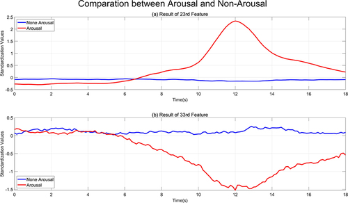
Furthermore, as illustrated in Figure 2, which depicts the timing fitness of sleep stages, this paper selects two features that are the most prominent: the duration of the frequency band for beta waves (feature number 23) and the local entropy for theta waves (feature number 33). Since the range of values for each feature is not uniform, standardization is performed to map to the range with a mean of 0 and a standard deviation of 1. The comparison of two feature value patterns during arousal and non-arousal sleep states is presented in Figure 11. The feature of duration of the frequency band for beta waves (feature number 23) is positively correlated with the arousal template, whereas the local entropy for theta waves (feature number 33) is negatively correlated. Both features are largely unrelated to the non-arousal signal.

Figure 11 Comparison between two features in arousal period. (a) is the correlation between the frequency band for beta waves (feature number 23) and the arousal template; (b) is the correlation between the local entropy for theta waves (feature number 33) and the arousal template.

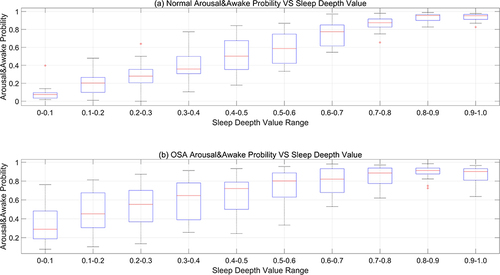
At the same time, this paper contrasts the likelihood of arousal during sleep between individuals with normal sleep patterns and patients with obstructive sleep apnea (OSA) in Figure 12. When the sleep depth value falls below 0.1 (indicating a state of deep sleep), the likelihood of arousal during sleep in individuals with normal sleep patterns is relatively low, exhibiting an average probability of less than 10%. Conversely, the mean arousal probability in OSA patients approximates 30%, aligning with the clinical observation that these patients frequently experience arousals and microarousals during sleep, which disrupts the normal sleep architecture and significantly diminishes sleep efficiency. Furthermore, regardless of normal sleep data or OSA sleep data, there is a pervasive trend: as the sleep depth value ascends (ranging from 0 to 1, indicating the transition from deep sleep to light sleep and then to wakefulness), the probability of arousal/wakefulness progressively increases.

Figure 12 Arousal & awake probability between normal and OSA. (a) represents the probability of experiencing arousal during sleep for individuals with normal sleep patterns; (b) denotes the likelihood of arousal events occurring during sleep in individuals diagnosed with obstructive sleep apnea (OSA).

Discussion

This paper establishes an artificial neural network model based on the sample values generated by the fusion of multiple sleep features. This model produces continuous sleep depth values (SDVs) ranging from 0 to 1, according to the multi-feature values at different time points during sleep. In doing so, we utilized a comprehensive set of features, including time-domain attributes, frequency-domain elements, and other relevant characteristics. The resulting sleep depth values generated by the model are capable of measuring the continuous variations in sleep depth and reflecting various aspects of sleep quality, such as the arousal/wakefulness index, the distribution of durations across different sleep stages, and overall sleep efficiency. During the development and validation of this model, it was found that the method of this paper has the following advantages:

1. Continuous Measurement: Unlike traditional sleep staging methods, which categorize sleep into discrete stages, this ANN model provides a continuous scale of sleep depth values (SDV) ranging from 0 (deep sleep) to 1 (wakefulness). Specifically, SDVs from 0 to 0.3 are associated with sleep, those ranging from 0.3 to 0.6 denote periods of unstable sleep, and values from 0.6 to 1 are indicative of wakefulness. This nuanced scale affords a more refined and granular insight into the dynamics of sleep state transitions and the subtleties of sleep patterns.

2. High Accuracy: The model demonstrates high accuracy in distinguishing between different sleep states, particularly in identifying wakefulness and deep sleep, which is crucial for applications where precise sleep state identification is necessary.

3. Accurate Arousal Measurement: The SDV is closely associated with the arousal/wakefulness index, making it a reliable indicator for predicting the transition between sleep states and the stability of sleep.

4. Flexible Model Application: The ANN model can be easily adapted to new data, enhancing its versatility. It can also function without additional training data, providing immediate sleep depth values that can streamline the process of sleep staging.

5. Potential for Real-Time Monitoring: With the ANN model, there is the possibility of real-time monitoring of sleep patterns, which could be particularly useful in clinical settings for assessing alertness levels or managing sedation during medical procedures.

Its disadvantages are:

Dependence on Technical Factors: The quality of the SDV calculation can be influenced by the data acquisition system and the algorithms used for signal processing, which may introduce variability or bias into the results.

Limitations in Application Process include:

1. Individual Differences: Although the Sleep Depth Value (SDV) demonstrates a strong correlation with sleep depth and arousability, there may be significant variability in SDV values among different individuals, which could affect the model’s ability to generalize across a diverse population. Further research may be needed to establish a normal range for SDV values.

2. Differentiation Between REM and NREM Sleep: Accurately differentiating between REM and NREM sleep stages may require additional data, such as electrooculogram (EOG) electrode readings, which are not considered within the scope of the current model.

3. Adaptability to Specific Applications: While the model shows promise in a controlled laboratory environment, its effectiveness in real-world applications, such as home monitoring or the treatment of sleep disorders, has yet to be fully determined and may require further validation.

Conclusion

This paper presents a pioneering design and calculation of the temporal fit of multiple features, forming statistical sample values of sleep depth based on feature values. It innovatively proposes and trains an artificial neural network model that can produce continuous sleep depth values ranging from 0 to 1 at any given moment (non-discrete values) and has validated the effectiveness of the model through various forms of verification. This model of sleep continuity can capture the nuances of the traditional five-stage classification method (W, N1, N2, N3, and REM) and subtle differences in microstates of sleep, considered as a complement or even an alternative to traditional sleep analysis. However, further research is needed to integrate it with other clinical outcomes.

Disclosure

The authors report no conflicts of interest in this work.

Acknowledgments

This study was supported the project of Shandong University Scientific Research Development Program (Grant No. J18KB071), Dongying Science and Technology Development Fund (Grant No. DJB2021010), Shandong Province Undergraduate Teaching Reform Research Project (Grant No. Z2021209 and Grant No. Z2023239) and Dongying Key Laboratory of Intelligent Information Processing and Sub-laboratory of Artificial Intelligence and Data Mining. Yunliang Sun and the Respiratory Department of Binzhou Medical University Hospital provided the data and gave a great help for paper writing and revision.

This paper has been facilitated and supported by the Biomedical Research Ethics Committee of Binzhou Medical University Affiliated Hospital: (1) Detailed explanations of the study were provided to participants, including the purpose, procedures, expected duration, potential risks and benefits, and any possible compensation. (2) Participants were ensured a full understanding of the information provided and had the opportunity to ask questions and discuss their concerns. (3) Voluntary participation was ensured, with participants knowing they could choose not to participate in the study or withdraw at any time without adverse consequences. (4) Completion of Patient Written Informed Consent. Prior to the commencement of the study, all participants were required to sign a written informed consent form. This form detailed all aspects of the study, including but not limited to the purpose, procedures, risks, benefits, and the methods of data collection and processing. (5) Participants were informed about how their personal information would be kept confidential and how the data would be securely stored and processed. (6) It was clearly explained to participants how their data would be used, including whether it would be shared with third parties and under what conditions. (7) Participants were informed of their right to receive updated information during the research process if there were any significant changes to the purpose, procedures, or risks of the study. (8) Communication with participants was maintained throughout the research process to ensure they continued to understand the progress and had the opportunity to ask questions or withdraw.

The research protocol of this study, including the methods of sleep data collection, has been reviewed and approved by the Biomedical Research Ethics Committee of the Affiliated Hospital of Binzhou Medical University. Throughout the research process, this study has continuously complied with the regulations and requirements set forth by the Ethics Review Committee, including the ethical principles outlined in the Declaration of Helsinki.

References

- Mellinger Glen D. Insomnia and its treatment. Arch Gen Psychiatry. 1985;42(3):225. doi:10.1001/archpsyc.1985.01790260019002
- Charbonnier S, Zoubek L, Lesecq S, Chapotot F. Self-evaluated automatic classifier as a decision-support tool for sleep/wake staging. Comput Biol Med. 2011;41(6):380–389. doi:10.1016/j.compbiomed.2011.04.001
- Geng D, Zhao J, Dong J, Jiang X, Gómez C, Schwarzacher SP. Comparison of support vector machines based on particle swarm optimization and genetic algorithm in sleep staging. Technol Health Care. 2019;27(S1):143–151. doi:10.3233/THC-199014
- Walthert L, Bauerfeind A, Kumar S. An automated random forest algorithm for sleep staging using advanced cardiorespiratory and movement features. Sleep Med. 2019;64(S1):S206–S206.
- Huang W, Guo B, Shen Y, et al. Sleep staging algorithm based on multichannel data adding and multifeature screening. Comput Methods Programs Biomed. 2020;187:105253. doi:10.1016/j.cmpb.2019.105253
- Hassan AR, Bhuiyan MIH. Automatic sleep stage classification. Paper presented at: International Conference on Electrical Information & Communication Technology; 2016.
- Jia-Yi GE, Peng Z, Xin Z, Hai-Ying L. Multiscale entropy analysis of EEG signal. Com Eng App. 2009;45(10):13–15.
- Larsen L, Walter D. Classification of sleep stages by EEG spectra; 1969.
- Vincent LC-F, Jaeseung J. Quantification of brain macrostates using dynamical nonstationarity of physiological time series. IEEE Trans Bio-Med Eng. 2011;58(4):1084–1093. doi:10.1109/TBME.2009.2034840
- Fraiwan L, Lweesy K, Khasawneh N, Wenz H, Dickhaus H. Automated sleep stage identification system based on time–frequency analysis of a single EEG channel and random forest classifier. Comput Methods Programs Biomed. 2012;108(1):10–19. doi:10.1016/j.cmpb.2011.11.005
- Weiss B, Clemens Z, Bódizs R, Halász P. Comparison of fractal and power spectral EEG features: effects of topography and sleep stages. Brain Res Bull. 2010;84(6):359–375. doi:10.1016/j.brainresbull.2010.12.005
- K D-K, K D, L J-G, W Y, J J. Deep learning application to clinical decision support system in sleep stage classification. Sleep Med. 2022;100(S1):136.
- Fernando -V-V, G-tg C, Eva C, et al. An explainable deep-learning model to stage sleep states in children and propose novel EEG-related patterns in sleep apnea. Comput Biol Med. 2023;165:107419. doi:10.1016/j.compbiomed.2023.107419
- R M, H R, K H, et al. Generalizable deep learning-based sleep staging approach for ambulatory textile electrode headband recordings. IEEE journal of biomedical and health informatics; 2023.
- Wei L, Lin Y, Wang J, Ma Y. Time-frequency convolutional neural network for automatic sleep stage classification based on single-channel EEG. In: 2017 IEEE 29th International Conference on Tools with Artificial Intelligence. IEEE; 2017.
- Emin TM, Necmettin S, Mehmet A. Estimation of sleep stages by an artificial neural network employing EEG, EMG and EOG. J Med Syst. 2010;34(4):717–725. doi:10.1007/s10916-009-9286-5
- Sors A, Bonnet S, Mirek S, Vercueil L, Payen J-F. A convolutional neural network for sleep stage scoring from raw single-channel EEG. Biomed Signal Process Control. 2018;42:107–114. doi:10.1016/j.bspc.2017.12.001
- Hsu Y-L, Yang Y-TC, Wang J-S, Hsu C-Y. Automatic sleep stage recurrent neural classifier using energy features of EEG signals. Neurocomputing. 2013;104:105–114. doi:10.1016/j.neucom.2012.11.003
- Akara S, Hao D, Chao W, Yike G. DeepSleepNet: a model for automatic sleep stage scoring based on raw single-channel EEG. IEEE Trans Neural Syst Rehabilit Eng. 2017;25(11):1998–2008. doi:10.1109/TNSRE.2017.2721116
- Jaemin J, Wonhyuck Y, JeongGun L, et al. Standardized image-based polysomnography database and deep learning algorithm for sleep stage classification. Sleep. 2023;46(12):zsad242.
- Dongrae C, Boreom L. Automatic sleep-stage classification based on residual unit and attention networks using directed transfer function of electroencephalogram signals. Biomed Sig Process Control. 2024;88(PB):105679.
- Helli M, Fortune RD. The neuronal transition probability (NTP) model for the dynamic progression of non-REM sleep EEG: the role of the suprachiasmatic nucleus. PLoS One. 2011;6(8):e23593.
- Uchida S, Maloney T, Feinberg I. Beta (20–28 Hz) and delta (0.3–3 Hz) EEGs oscillate reciprocally across NREM and REM sleep. Sleep. 1992;15(4):352–358. doi:10.1093/sleep/15.4.352
- Uchida S, Maloney T, March JD, Azari R, Feinberg I. Sigma (12–15 Hz) and delta (0.3–3 Hz) EEG oscillate reciprocally within NREM sleep. Brain Res Bull. 1991;27(1):93–96. doi:10.1016/0361-9230(91)90286-S
- Pardey J, Roberts S, Tarassenko L, Stradling J. A new approach to the analysis of the human sleep/wakefulness continuum. J Sleep Res. 2010;5(4):201–210. doi:10.1111/j.1365-2869.1996.00201.x
- Asyali MH, Berry RB, Khoo MCK, Altinok A. Determining a continuous marker for sleep depth. Comput Biol Med. 2007;37(11):1600–1609. doi:10.1016/j.compbiomed.2007.03.001
- Magdy Y, Michele O, Marc S, et al. Odds ratio product of sleep EEG as a continuous measure of sleep state. Sleep. 2015;38(4):641–654. doi:10.5665/sleep.4588
- Magdy Y, Ali A, Michelle R, Md R, Susan R. Characteristics and reproducibility of novel sleep EEG biomarkers and their variation with sleep apnea and insomnia in a large community-based cohort. Sleep. 2021;44(10):zsab145.
- Magdy Y, Bethany G, Pack AI, Kuna ST, Cecilia C, Susan R. Sleep architecture based on sleep depth and propensity: patterns in different demographics and sleep disorders and association with health outcomes. Sleep. 2022;45(6):zsac059.
- Magdy Y, Bethany G, Eleni G, et al. Contribution of obstructive sleep apnea to disrupted sleep in a large clinical cohort of patients with suspected OSA. Sleep. 2023;46(7):zsac321.
- Bethany G, Ks T, Allan P, et al. An approach for determining the reliability of manual and digital scoring of sleep stages. Sleep. 2023;46(11):zsad248.
- Sultan Q, Hani M, Faris A, et al. The prevalence of rapid eye movement-related obstructive sleep apnea in a sample of Saudi population. Ann Thorac Med. 2023;18(2):90–97. doi:10.4103/atm.atm_388_22
- Anna R, Cs L, Fan H, et al. Association of a novel EEG metric of sleep depth/intensity with attention-deficit/hyperactivity, learning and internalizing disorders and their pharmacotherapy in adolescence. Sleep. 2021;45(3):zsab287.
- Julio FM, Anna R, Fan H, et al. 0254 association of slow wave activity and odds ratio product with internalizing and externalizing problems in children and adolescents. Sleep. 2022(Supplement_1):A114.