A simulation of cross-country skiing on varying terrain by using a mathematical power balance model

Abstract

The current study simulated cross-country skiing on varying terrain by using a power balance model. By applying the hypothetical inductive deductive method, we compared the simulated position along the track with actual skiing on snow, and calculated the theoretical effect of friction and air drag on skiing performance. As input values in the model, air drag and friction were estimated from the literature, whereas the model included relationships between heart rate, metabolic rate, and work rate based on the treadmill roller-ski testing of an elite cross-country skier. We verified this procedure by testing four models of metabolic rate against experimental data on the treadmill. The experimental data corresponded well with the simulations, with the best fit when work rate was increased on uphill and decreased on downhill terrain. The simulations predicted that skiing time increases by 3%–4% when either friction or air drag increases by 10%. In conclusion, the power balance model was found to be a useful tool for predicting how various factors influence racing performance in cross-country skiing.

Keywords:

• skiing
• power balance
• metabolic rate
• work rate
• air drag
• friction coefficient

Introduction

Cross-country skiing is physically demanding, technically complex, and performed on varying terrain and at widely varying speeds.^1,2 In most races, approximately one-third of the distance is performed on uphill, flat, and downhill terrain, respectively, and a skier must alter his technique and work rate according to the incline, snow friction, and air drag.^2–4 To successfully overcome these demands, cross-country skiers require high metabolic rates,^5–7 good ability to convert metabolic rate into work rate and speed,⁸ and low snow friction and air drag. During competitions, elite cross-country skiers work at higher metabolic rates on uphill compared to downhill terrain,^9,10 and are also found to produce the highest work rates on uphill terrain;⁴ Norman et al 1989.¹¹ Work rates on downhill terrain have not yet been examined due the difficulties of measuring snow friction and air drag on this terrain. The exact importance of snow friction and air drag during competitions at varying speeds is examined in this paper.

A better understanding (compared with what is currently available in the literature) of how physiological and mechanical factors interact in influencing cross-country skiing performance may be gained by using a power balance model. The power balance equation relates power production and power dissipation, and has been shown to be successful for predicting performance in running, cycling, and speed skating.^12–14 More recently, the equation has been used on cross-country skiing.^11,15 In cross-country skiing a numerical simulation of a ski race was also recently developed by Carlsson et al.¹⁶ The authors included gravitational force, normal force between snow and skis, drag force from the wind, frictional force between snow and skis, and driving force from the skier in the simulation. However, their outcomes were not compared with experimental results. The new insights provided in this paper are to show whether it is possible to accurately predict the experimental position on uphill and downhill terrain and if the skier’s power changes with the terrain. Predicting the position presupposes knowing the work rate and relevant input data during skiing, or estimating the work rate prior to skiing based on earlier skiing and knowledge of personal characteristics. We suggest three methods for determining the work rate: first (method A), determining the work rate from VO₂(t) and VCO₂(t); second (method B), determining the work rate from VCO₂(t) and heart rate; third (method C), determining the work as a function of the heart rate. We define performance as being inverse and proportional to the time by which the skier completes a given track.

Extending Carlsson et al’s¹⁶ research, the aims of this paper were to simulate cross-country skiing on varying terrain by using a power balance model, compare a skier’s simulated position along the track with the experimental position when skiing on snow, and calculate the theoretical effect of changed friction or air drag on skiing performance. We hypothesize that the model can provide accurate predictions of the position along the track during cross-country skiing on varying terrain.

Basic definitions

Metabolic rate Q is the total energy used by the body per time unit. Work rate P is the external work produced per time unit.

Methods

Overall design

A skier’s position along the track during ski skating on varying terrain was simulated using a power balance model relating power production and power dissipation. The simulations were performed in Mathematica 9 (Wolfram Research, Inc, Champaign, IL, USA). As input values in the model, air drag and friction were estimated from the literature, whereas the model included relationships between heart rate p, metabolic rate Q, and work rate P based on treadmill roller ski testing of an elite cross-country skier. Because metabolic rate was based on heart rate in the simulations on the terrain, we verified this procedure by testing four models of metabolic rate against experimental data obtained on the treadmill. The simulation was compared to actual skiing in a competition track on varying terrain by employing the skating technique. Finally, we simulated the theoretical effect of changed friction and air drag on the position along the track using the model.

Power balance equation

A skier’s rate of change in kinetic energy (E_k) equals body mass (m) multiplied with speed (v) and acceleration (dv/dt) where t is time. van Ingen Schenau and Cavanagh’s¹⁷ power balance equation states that

$\underset{Rateofchangofkineticenergyofskier}{\underbrace{d(E_k)/dt}}=mv\frac{dv}{dt}=\underset{Locomotivepower}{\underbrace{P}}-\underset{Frictionpower}{\underbrace{\mu mgCos(\alpha )v}}-\underset{Gravitationalpower}{\underbrace{mgSin(\alpha )v}}-\underset{Airdragpower}{\underbrace{\frac{1}{2}\rho C_{d}A{v}^3}}$(1)

where P is the work rate (also called locomotive power), μ is the friction coefficient, g is the gravitational acceleration, ρ is the air density, C_d is the drag coefficient, and A is the projected front area of the skier (m²). In addition, α is the angle of inclination measured in radians between a tangent of the track and the horizontal level. Therefore,

$Tan(\alpha )=dh(s)/dx,$(2)

where h(s) is the height of the terrain relative to the starting point as a function of the accumulated distance s along the terrain from the beginning of the track and x is the horizontal position. Thus π/4 ≈ 0.79, which means 45 degrees upward incline and π/2 ≈ 1.57, which means vertical upward incline. We used straight lines between points, which indicates a piecewise linear track. Geometrical considerations give

$dh(s)/dx=(dh/ds)/\sqrt{1-{(dh/ds)}^2}.$(3)

Thus,

$\alpha =ArcTan(dh/ds)=ArcTan\left((dh/ds)/\sqrt{1-{(dh/ds)}^2}\right).$(4)

For the relatively small angles of inclinations used in the current study,

$Tan(\alpha )\approx Sin(\alpha )\approx \alpha .$(5)

In Equation 1$\underset{Rateofchangofkineticenergyofskier}{\underbrace{d(E_k)/dt}}=mv\frac{dv}{dt}=\underset{Locomotivepower}{\underbrace{P}}-\underset{Frictionpower}{\underbrace{\mu mgCos(\alpha )v}}-\underset{Gravitationalpower}{\underbrace{mgSin(\alpha )v}}-\underset{Airdragpower}{\underbrace{\frac{1}{2}\rho C_{d}A{v}^3}}$(1) ,m, v, A, P, and E_k are physiological and μ, C_d, ρ, α, and g are mechanical. The work rate P in Equation 1$\underset{Rateofchangofkineticenergyofskier}{\underbrace{d(E_k)/dt}}=mv\frac{dv}{dt}=\underset{Locomotivepower}{\underbrace{P}}-\underset{Frictionpower}{\underbrace{\mu mgCos(\alpha )v}}-\underset{Gravitationalpower}{\underbrace{mgSin(\alpha )v}}-\underset{Airdragpower}{\underbrace{\frac{1}{2}\rho C_{d}A{v}^3}}$(1) correlates with all these parameters and variables. Sandbakk et al^11,18,19 have shown how work rate is related to metabolic rate, incline, and technique. For example, elite skiers demonstrate higher work rates on uphill terrain, employing higher cycle rates and more work per cycle in association with a longer relative propulsive phase.

Model assumptions and laboratory testing

In order to optimize the simulation of actual skiing on snow for an individual skier, the model developed below includes relationships between heart rate, metabolic rate Q, and work rate P based on treadmill roller ski testing where the researchers studied how heart rate and metabolic rate are altered when skiing on varying terrain. We applied an elite male skier with the following characteristics: 31 years old body mass of 77.5 kg, height of 182 cm, maximal oxygen intake (VO₂ max) of 70 mL × kg/minute, has competed at the national and international levels for over 10 years, and currently trains in skiing for 500 hours per year. When repeating the experiment with this elite skier, our experience is that the difference for the measured variables would not be larger than 2%, which we consider to be an upper bound error margin. Since skiers are not alike, it is better to use one experienced skier than a set of different skiers to collect aggregated data suitable for this particular skier. Although we consider the elite skier to be representative of elite skiers, other elite skiers with different characteristics will generate different aggregated data and behave differently. The model constitutes a tool that can be applied by different skiers.

The elite skier performed three different test protocols while roller skiing on a treadmill at standardized conditions from which input values were collected. Equipment and procedures were similar to the studies by Sandbakk et al,⁸ and the roller skis used on the treadmill tests were tested for rolling friction force (N) in a towing test, as previously described.⁸ The friction coefficient was determined by dividing rolling friction force by the normal force, and the mean friction coefficient (0.024) was incorporated in the work rate (P) calculations. Respiratory parameters were assessed employing open-circuit indirect calorimetry with an Oxycon Pro apparatus (Jaeger GmbH, Hoechberg, Germany). Heart rate (beats per minute [bpm]) was determined with a heart rate monitor (Polar RS800; Polar Electro OY, Kempele, Finland) and blood lactate concentration (mmol/L) in 5 μL samples of blood were taken from a fingertip and was quantified using a Lactate Pro LT-1710t kit (ARKRAY, Inc, Kyoto, Japan).

First, a treadmill test was used to define the relationships between work rate and metabolic rate Q at different inclines. The skier was tested at various speeds on the four angles of inclination (0.02, 0.05, 0.08, and 0.12 radians). Five-minute stages were applied for each speed on each angle of inclination α. The break between each stage was 2 minutes. The speeds were 4.72 m/second for the angle of inclination of 0.02 radians; then 2.78 m/second, 3.89 m/second, 4.44 m/second, 5.0 m/second, and 6.5 m/second for the angle of inclination of 0.05 radians; then 2.5 m/second for the angle of inclination of 0.08 radians; and finally 1.94 m/second, 2.22 m/second, and 2.50 m/second for the angle of inclination of 0.12 radians. The skier used a self-chosen skating technique (ie, G3 at the angles of inclinations of 0.02 radians, 0.05 radians, and 0.08 radians, and G2 at the angles of inclination of 0.12 radians) and cycle rate. G3 is used on moderate angles of inclination and level terrain, and it is also called double dance, V2, and 1-skate. G2 is a technique for skiing uphill and is also called V1. Metabolic rate in Joules per second (J/s) was determined from the rate of oxygen consumption (VO₂) and the rate of carbon dioxide production (VCO₂) according to the relation by Tokui and Hirakoba,²⁰

$Q_A(t)=\left(0.0862\cdot \left(Min\left(R_q(t),1\right)\right)+0.267\right)\cdot V{O}_2(t)$(6)

where R_q(t) = VCO₂(t)/VO₂(t) is the ratio of VCO₂ produced to VO₂ consumed at the cellular level, and Min(R_q(t),1) gives R_q(t) if R_q(t) < 1, and Min(R_q(t),1) gives 1 otherwise.

In the calculations of work rate P, air drag is not present on the treadmill and

$d(E_k)/dt=1/2\rho C_{d}A{v}^3=0$(7)

during steady state. Therefore, work rate P from Equation 1$\underset{Rateofchangofkineticenergyofskier}{\underbrace{d(E_k)/dt}}=mv\frac{dv}{dt}=\underset{Locomotivepower}{\underbrace{P}}-\underset{Frictionpower}{\underbrace{\mu mgCos(\alpha )v}}-\underset{Gravitationalpower}{\underbrace{mgSin(\alpha )v}}-\underset{Airdragpower}{\underbrace{\frac{1}{2}\rho C_{d}A{v}^3}}$(1) is given by

$P=\mu mgCos(\alpha )v+mgSin(\alpha )v.$(8)

A second treadmill test was performed at incremental speeds at an angle of inclination α of 0.05 radians to assess the VO₂ max. This test was considered to represent maximal effort if the following three criteria were met: (1) a plateau in VO₂ with increasing exercise intensity; (2) a respiratory exchange ratio (ie, rate of carbon dioxide production divided by the rate of oxygen consumption, greater than 1.10); and (3) blood lactate concentration exceeding 8 mmol·L⁻¹. VO₂ was measured continuously and the average of the three highest consecutive 10-second values designated as the VO₂ max. A VO₂ max of 5343 mL/minute was measured from which the maximal metabolic rate was calculated when inserting R_q(t) = 1 into Equation 6$Q_A(t)=\left(0.0862\cdot \left(Min\left(R_q(t),1\right)\right)+0.267\right)\cdot V{O}_2(t)$(6) , which gives

$Q_{A\max }=(0.0862+0.267)\cdot V{O}_2\max =1887J/s.$(9)

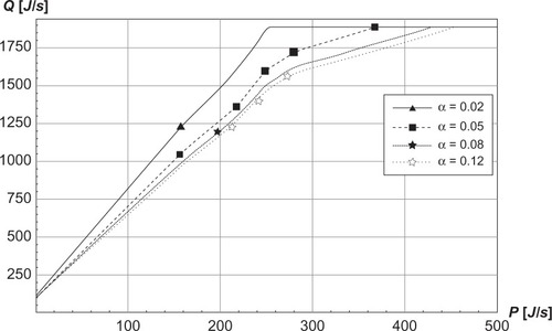
Work rate P and metabolic rate Q for the 5-minute stages during steady state and Q_Amax are plotted in Figure 1.

Figure 1 Metabolic rate Q (P, α) as a function of work rate P for angles of inclinations of α = 0.02 radians (upper line), 0.05 radians, 0.08 radians, and 0.12 radians (lower line) while treadmill roller-skiing using the skating technique.

Notes: The curve fittings are based on linear interpolation through the experimental points. Metabolic rate of zero work rate Q₀ = 332 J/s. Maximal metabolic rate Q_Amax = 1887 Joules per second (J/s) (represented by a straight upper line). ★: Experimental values for α = 0.02 radians. ■: Experimental values for α = 0.05 radians. ☆: Experimental values for α= 0.08 radians. ▲: Experimental values for α = 0.12 radians.

In order to investigate the relationship between work rate P and metabolic rate Q at different angles of inclination the following seven assumptions were made.

Assumption A: steady state exercise is considered (ie, dv/dt = 0).

Assumption B: The metabolic rate Q during steady state for a given technique is an invertible function of work rate P and angle of inclination α, that is,

$Q=Q(P,\alpha )\iff P=P(Q,\alpha ).$(10)

We do not postulate cause and effect relationships between Q and P; we simply assume that one is a function of the other. Explicit dependencies of metabolic rate Q on the friction coefficient, body mass, air drag, and cycle length were not assumed. In principle, cycle rate and technique vary with angle of inclination and speed.^21,22 However, we assume that an individual skier will voluntarily prefer the most economical cycle rate for a chosen technique.

Assumption C: the metabolic rate Q is the sum of the metabolic rate of unloaded skiing Q₀ and the metabolic rate of loaded skiing Q_L, ie,

$Q\stackrel{def}{=}{Q}_0+Q_L.$(11)

The metabolic rate of unloaded skiing is the energy cost at a zero work rate Q₀, which is determined by the rate of resting metabolism together with the energy required for unloaded movement of body segments. More specifically, the metabolic rate of unloaded skiing accounts for all metabolic rate, except for the additional metabolic rate used to generate work against gravitation, friction, and air drag. This additional metabolic rate is the metabolic rate of loaded skiing Q_L, which is the difference between the total energy cost and the energy cost of unloaded skiing.

Assumption D: the metabolic rate of unloaded skiing Q₀ depends neither on work rate P, nor on the angle of incline α.

Assumption E: the metabolic rate of loaded skiing depends multiplicatively on two functions, which depend on the work rate P and the angle of inclination α, ie,

$Q_L=Q_1^{0.05}(P)\cdot \lambda (\alpha ).$(12)

Assumption F: the function $Q_1^{0.05}(P)$, which plays a role in loaded skiing, is a strictly increasing function of the work rate P for an angle of incline of α = 0.05 radians, ie, $\partial Q_1^{0.05}(P)/\partial P>0$.

We consider α = 0.05 radians as a suitable uphill incline to ensure the proper impact of loaded skiing. In this paper, we define uphill as above 0.02 radians and downhill as below −0.02 radians. Intuitively, the higher work rate P gives higher metabolic rate Q. Further, α = 0.05 radians is a typical angle of inclination used for test protocols during roller skiing. Substantial amounts of data exist for this angle of inclination α. We chose piecewise linearity for $Q_0+Q_1^{0.05}(P)$ in the empirical testing, since we have too few data points for the least squares fit method here.

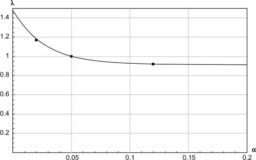
Assumption G: the function λ (α) impacting QL in loaded skiing is a convexly decreasing function of the angle of inclination (α), ie, ∂λ(α)/∂α < 0, ∂²λ(α)/∂α² > 0, where we choose the functional form

$\lambda \left(\alpha \right)=c_1\left(1+c_{2}Exp\left(-c_3\alpha \right)\right),$(13)

where c₁, c₂, and c₃ are positive parameters.

The decreasing λ(α) is justified by Sandbakk et al,¹⁹ who showed that an increasing angle of inclination α causes higher work rate P for the same metabolic rate Q, due to higher cycle rates and more work per cycle on uphill terrain, which was associated with longer relative propulsive phases at shorter recovery times during a cycle at steeper inclines. This is in agreement with what is experienced when running or walking. See Margaria et al²³ for further discussions concerning this issue. The parameters c₁, c₂, and c₃ are estimated in Supplementary materials.

In order to assess the nature of the seven assumptions, we would first like to establish a model for the skier’s work rate P, which enables us to simulate the position of the center of mass as a function of time. This is similar to Newton’s approach when he forecasted the law of gravitation, where the deduction that followed was that the position of the center of mass of the planets as a function of time was tested. Analogously, we compare the simulated and experimental position time history of the skier. Notable is that Newton could not give any explanation for why the gravitational force should go as 1/r². The same applies for P in the current study.

Consistent with these seven assumptions, we assume that the metabolic rate Q during a steady state is determined by

$\begin{array}{l}Q(P,\alpha )=Q_0+Q_1^{0.05}(P)\cdot \lambda (\alpha ),\hfill \\ \lambda (\alpha )=0.91(1+0.62e^{-37.59\alpha })\hfill \end{array}$(14)

Figure 1 shows how Equation 14$\begin{array}{l}Q(P,\alpha )=Q_0+Q_1^{0.05}(P)\cdot \lambda (\alpha ),\hfill \\ \lambda (\alpha )=0.91(1+0.62e^{-37.59\alpha })\hfill \end{array}$(14) fits to the data for the angles of inclination of 0.02 radians, 0.05 radians, 0.08 radians, and 0.12 radians. Figure 2 shows the function λ(α). We consider work rate P and angle of inclination (α) to be functions of time (t), and write Q(t) = Q(P[t], α[t]).

Figure 2 The λ(α) function in Equation 14$\begin{array}{l}Q(P,\alpha )=Q_0+Q_1^{0.05}(P)\cdot \lambda (\alpha ),\hfill \\ \lambda (\alpha )=0.91(1+0.62e^{-37.59\alpha })\hfill \end{array}$(14) where λ(α) is a convexly decreasing function of the angle of inclination α.

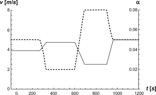
We conducted a third treadmill test in order to analyze how well different equations for the relationships between work rate P and metabolic rate Q correlated, accounting for different speeds and inclines. In this test, speed and the angle of inclination on the treadmill were varied according to Figure 3 with VO₂(t) and VCO₂(t) in mL/minute, and heart rate p(t) in bpm, measured continuously every 30 seconds during the test. The skier always used the G3 technique.

Figure 3 Speed v and angle of inclination α as functions of time t while treadmill roller-skiing using the skating technique.

Notes: Solid line: the skier’s speed v in m/second as a function of time t in seconds. Dashed line: the treadmill’s angle of inclination α in radians as a function of time t in seconds.

These data allow us to model the metabolic rate Q using three alternative methods: A, B, and C. The first method (A) uses the experimentally measured VO₂(t) and VCO₂(t) and Equation 6$Q_A(t)=\left(0.0862\cdot \left(Min\left(R_q(t),1\right)\right)+0.267\right)\cdot V{O}_2(t)$(6) . The second method (B) uses the experimentally measured VCO₂(t) and heart rate p(t), but not VO₂(t), and assumes a linear relationship between heart rate p(t) and the rate of oxygen consumption as traditionally used in the literature.²⁴

$V{O}_{2B}(t)=V{O}_{2b}+\frac{(V{O}_2\max -V{O}_{2b})}{p_{\max }-p_b}\cdot \left(p(t)-p_b\right)$(15)

where VO_2b is the oxygen consumption during the rest set to 240 mL/minute rate of oxygen consumption, VO₂ max is the maximal rate of oxygen consumption set to 5343 mL/minute, p_b is the resting heart rate of 42 bpm, and p_max is the maximal heart rate of 195 bpm. Equation 15$V{O}_{2B}(t)=V{O}_{2b}+\frac{(V{O}_2\max -V{O}_{2b})}{p_{\max }-p_b}\cdot \left(p(t)-p_b\right)$(15) , which is based on heart rate, gives the oxygen consumption VO_2B(t), which may differ from the VO₂(t) measured experimentally. Using VO_2B(t) instead of VO₂(t) in Equation 6$Q_A(t)=\left(0.0862\cdot \left(Min\left(R_q(t),1\right)\right)+0.267\right)\cdot V{O}_2(t)$(6) gives

$Q_B(t)=\left(0.0862\cdot \left(Min\left(R_{qB}(t),1\right)\right)+0.267\right)\cdot \left(V{O}_{2b}+\frac{\left(V{O}_2\max -V{O}_{2b}\right)}{\left(p_{\max }-p_b\right)}\cdot \left(p(t)-p_b\right)\right)$(16)

where R_qB(t) = VCO₂/VO_2B(t).

The third method (C) accounts for a time lag τ of 30 seconds before oxygen consumption reaches a steady state. We assume the first order differential equation

$\frac{d{Q}_C(t)}{dt}=\frac{\left(Q(t)-Q_C(t)\right)}{\tau }$(17)

where Q(t) is determined by Equation 14$\begin{array}{l}Q(P,\alpha )=Q_0+Q_1^{0.05}(P)\cdot \lambda (\alpha ),\hfill \\ \lambda (\alpha )=0.91(1+0.62e^{-37.59\alpha })\hfill \end{array}$(14) ,Q_C(t₀) = 80 J/sτ = 30 s. During the steady state work rate P, Equation 17$\frac{d{Q}_C(t)}{dt}=\frac{\left(Q(t)-Q_C(t)\right)}{\tau }$(17) produces an exponential function for Q_C(t), which is reminiscent of the exponential curve plots suggested by di Prampero.²⁵ The metabolic rate Q(P,α) in Equation 14$\begin{array}{l}Q(P,\alpha )=Q_0+Q_1^{0.05}(P)\cdot \lambda (\alpha ),\hfill \\ \lambda (\alpha )=0.91(1+0.62e^{-37.59\alpha })\hfill \end{array}$(14) applies for a steady state and gives a poor prediction in a nonsteady state. However, Q_C(t) in Equation 17$\frac{d{Q}_C(t)}{dt}=\frac{\left(Q(t)-Q_C(t)\right)}{\tau }$(17) is a function of work rate P, angle of inclination α, time t and the time lag τ, and also gives a good prediction in a nonsteady state.

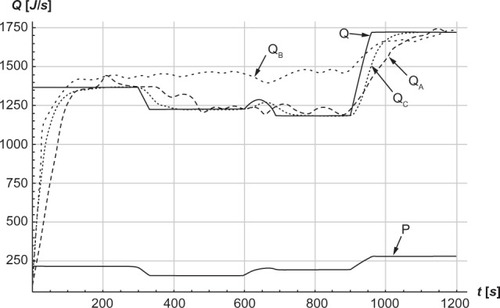
In Figure 4, Q_B(t) is different from Q_A(t). The reason for this is that Q_B(t), which is calculated from the heart rate, tends to drift from around 300 seconds, which most likely can be explained by thermal heating that drifts the heart rate. Since Q_B(t) and Q_A(t) differ, caution is needed when applying VO₂(t) versus heart rate p(t) to estimate metabolic rate.

Figure 4 Calculations of work rate P and metabolic rates Q as functions of time t in Joules per second (J/s).

Steady state

On the four plateaus in Figure 4, which correspond to the four work rates tested we get steady state conditions with constant metabolic rate. Inserting dQ_C(t)/dt = 0 into Equation 17$\frac{d{Q}_C(t)}{dt}=\frac{\left(Q(t)-Q_C(t)\right)}{\tau }$(17) leads to Q(t) = Q_C(t). Figure 4 shows that Q_A(t) is in good agreement with Q(t) on the plateaus (ie, Q_A(t) ≈ Q(t) = Q_C(t)). This agreement is notable since it was not built into the models from the beginning. Q(t) was developed in Equation 14$\begin{array}{l}Q(P,\alpha )=Q_0+Q_1^{0.05}(P)\cdot \lambda (\alpha ),\hfill \\ \lambda (\alpha )=0.91(1+0.62e^{-37.59\alpha })\hfill \end{array}$(14) using the least squares fit method in Supplementary materials on the ten experimental points in Figure 1. Q_A(t) was developed in Equation 6$Q_A(t)=\left(0.0862\cdot \left(Min\left(R_q(t),1\right)\right)+0.267\right)\cdot V{O}_2(t)$(6) using VO₂(t) as the experimental input causing the four experimental points on the plateaus in Figure 4.

Kinematic state

Equation 14$\begin{array}{l}Q(P,\alpha )=Q_0+Q_1^{0.05}(P)\cdot \lambda (\alpha ),\hfill \\ \lambda (\alpha )=0.91(1+0.62e^{-37.59\alpha })\hfill \end{array}$(14) was constructed by assuming steady state, but work rate P and the angle of inclination α vary through time t when cross-country skiing on the terrain. Thus, cross-country skiing is generally not performed at a steady state (for example, due to downhill sections). Q_A(t), Q_B(t), and Q_C(t) are not based on a steady state and apply generally. Figure 4 shows that the third treadmill test strongly supports our model for Q_C(t) and Q(P, α). Q_A(t) is somewhat delayed compared to Q_C(t), which is explained by the measuring apparatus of VO₂(t) used for Q_A(t), which shows an inherent time lag of around 15 seconds.

Equation 17$\frac{d{Q}_C(t)}{dt}=\frac{\left(Q(t)-Q_C(t)\right)}{\tau }$(17) is not invertible to determine P(t), but by measuring the heart rate p(t) on the terrain, Q_B(t) can be determined and compared with Q_C(t). Thus, an estimate for the work rate P(t) can be inferred in future research.

Comparing simulated cross-country skiing with experimental data

As done many times earlier in sports analysis, we modeled the moving system (ie, the skier) with particle mechanics. We modeled the motion of the center of mass of a skier on the terrain where the skier’s air drag depends on the projected front area. One difference between solid state physics and biomechanics is that the skier is not a rigid object, which means that the center of mass is not at a fixed position in the body. However, the center of mass can be found from the geometrical configuration of the skier, and the position time history can be compared with simulations of the center of mass position versus time.

By using the power balance model, 5 km cross-country skiing on varying terrain was simulated. The track profile is shown in Figure 5, where the 16 filled squares are the time measurements for the skier along the track, and the 58 stars are the height points. A straight line is drawn between each star. The model is solved for each straight line. As input to the power balance model, air drag and friction were estimated from the literature, whereas relationships between heart rate, metabolic rate, and work rate were determined from the treadmill roller ski tests. The skier mainly used the G3 technique. The skier warmed up for 20 minutes at a low intensity before skiing. His starting heart rate was 120 bpm. Research assistants measured time using synchronized stop watches when the skier passed the defined points along the track. These defined points were chosen based on significant changes in the track profile and so that the research assistants could see the skier in good time before passing the point. Heart rate was followed continuously with the Polar RS800 heart rate monitor (Polar Electro OY).

Figure 5 Height h as a function of distance s in meters along the track.

Notes: ★: 58 height measurement points. Straight lines are drawn between each star, which indicates a piecewise linear track. ■: 16 points where time measurements were made.

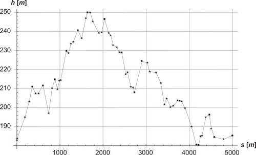
The skiing terrain is described by height h in meters as a function of distance s in meters along the terrain and used as input to the simulations. Supplementary materials specifies how distances along the track were measured, and identifies the associated uncertainties. A constant friction coefficient μ of 0.037 was applied in the calculations of work rate P. This friction coefficient was based on findings for snow conditions similar to those on the test day with old grained snow (enabling fast skiing) and minus 2–3°C. On such conditions, the friction coefficient is minimal assuming independence between speed and body weight.^26,27 Air drag depends on the size and position of the skier. Based on estimates from the measured forces in Leirdal et al,²⁸ air drag was estimated to be C_dA = 0.45 m² in upright posture (which is comparable to upright skating on flat and uphill terrain) and C_dA = 0.39 m² in a semisquatting posture (comparable to skating without poles used on downhill terrain). Spring et al²⁹ reported values as high as 0.6–0.7 m² for upright positioning and as low as 0.27–0.33 m² in a deep tuck position. These numbers are conflicting, which we resolved as follows: to account for air drag, C_dA = 0.4 m² was employed on the terrain since the skier used upraised or semisquatting postures most of the time.

Equation 1$\underset{Rateofchangofkineticenergyofskier}{\underbrace{d(E_k)/dt}}=mv\frac{dv}{dt}=\underset{Locomotivepower}{\underbrace{P}}-\underset{Frictionpower}{\underbrace{\mu mgCos(\alpha )v}}-\underset{Gravitationalpower}{\underbrace{mgSin(\alpha )v}}-\underset{Airdragpower}{\underbrace{\frac{1}{2}\rho C_{d}A{v}^3}}$(1) can be divided by v to give an equation of the skier’s motion. This gives

$\begin{array}{l}m\frac{dv}{dt}=P/v(t)-mgSin\left(\alpha (s(t))\right)-mg\mu Cos\left(\alpha (s(t))\right)-\frac{1}{2}\rho C_{d}Av{(t)}^2,\hfill \\ \frac{ds}{dt}=v(t),\hfill \end{array}$(18)

which is applicable for a constant slope. Equation 18$\begin{array}{l}m\frac{dv}{dt}=P/v(t)-mgSin\left(\alpha (s(t))\right)-mg\mu Cos\left(\alpha (s(t))\right)-\frac{1}{2}\rho C_{d}Av{(t)}^2,\hfill \\ \frac{ds}{dt}=v(t),\hfill \end{array}$(18) is solved numerically, as two coupled, nonlinear, ordinary differential equations in order to find the accumulated distance s(t) from the beginning of the track and the speed v(t) of the skier as a function of time; s(t) was compared with the experimental results. Equations 1$\underset{Rateofchangofkineticenergyofskier}{\underbrace{d(E_k)/dt}}=mv\frac{dv}{dt}=\underset{Locomotivepower}{\underbrace{P}}-\underset{Frictionpower}{\underbrace{\mu mgCos(\alpha )v}}-\underset{Gravitationalpower}{\underbrace{mgSin(\alpha )v}}-\underset{Airdragpower}{\underbrace{\frac{1}{2}\rho C_{d}A{v}^3}}$(1) and 18$\begin{array}{l}m\frac{dv}{dt}=P/v(t)-mgSin\left(\alpha (s(t))\right)-mg\mu Cos\left(\alpha (s(t))\right)-\frac{1}{2}\rho C_{d}Av{(t)}^2,\hfill \\ \frac{ds}{dt}=v(t),\hfill \end{array}$(18) are referred to as the power balance model.

The experimental results were tested against two different assumptions for the work rate P as an input to the power balance model. The first assumption was that a constant work rate P, based on average metabolic rate Q, was calculated from the average heart rate p along the track. This average heart rate was recorded as 0.823 p_max. R_q(t) was assumed to be 1.0 based on treadmill testing at this exercise intensity. Equation 16$Q_B(t)=\left(0.0862\cdot \left(Min\left(R_{qB}(t),1\right)\right)+0.267\right)\cdot \left(V{O}_{2b}+\frac{\left(V{O}_2\max -V{O}_{2b}\right)}{\left(p_{\max }-p_b\right)}\cdot \left(p(t)-p_b\right)\right)$(16) gives Q_B = 1480 J/s in this case. Figure 5 shows that the track increases from (s, h) = (0, 183) to (s, h) = (1700, 250) over the first 1700 m which gives α = 0.04 radians as the average angle of inclination. The work rate P during uphill skiing was calculated by using α = 0.04. Combining Equations 16$Q_B(t)=\left(0.0862\cdot \left(Min\left(R_{qB}(t),1\right)\right)+0.267\right)\cdot \left(V{O}_{2b}+\frac{\left(V{O}_2\max -V{O}_{2b}\right)}{\left(p_{\max }-p_b\right)}\cdot \left(p(t)-p_b\right)\right)$(16) and 14$\begin{array}{l}Q(P,\alpha )=Q_0+Q_1^{0.05}(P)\cdot \lambda (\alpha ),\hfill \\ \lambda (\alpha )=0.91(1+0.62e^{-37.59\alpha })\hfill \end{array}$(14) gives P = P(Q,α) = P(1480,0.04) = 225 J/s. Downhill work rates P are not yet investigated in cross-country skiing, and 225 J/s was therefore used on all angles of inclinations in a first model.

The second assumption for the work rate P was based on the observed differences in heart rate on uphill and downhill terrain. The skier’s heart rate corresponded to around 90% of VO₂ max uphill (above 0.02 radians uphill), around 80% on flat terrain, and around 70% downhill (below −0.02 radians downhill). As the current track profile contained almost purely uphill and downhill terrain, 90% of the VO₂ max on uphill sections, 80% on the flat sections, and 70% of the VO₂ max on downhill sections were implemented. Combining Equations 16$Q_B(t)=\left(0.0862\cdot \left(Min\left(R_{qB}(t),1\right)\right)+0.267\right)\cdot \left(V{O}_{2b}+\frac{\left(V{O}_2\max -V{O}_{2b}\right)}{\left(p_{\max }-p_b\right)}\cdot \left(p(t)-p_b\right)\right)$(16) and 14$\begin{array}{l}Q(P,\alpha )=Q_0+Q_1^{0.05}(P)\cdot \lambda (\alpha ),\hfill \\ \lambda (\alpha )=0.91(1+0.62e^{-37.59\alpha })\hfill \end{array}$(14) gives a metabolic rate Q_B = Q = 1656 J/s and a work rate P = 253 J/s on uphill terrain, and a metabolic rate Q_B = Q = 1285 J/s and a work rate P = 253 × 0.7/0.9 = 197 J/s on downhill terrain. Supplementary materials tests how the simulations fit with the experimental data.

As a final simulation based on the second assumption for work rate P, effects of changed friction and air drag on the position along the track and on total skiing time were simulated. Here, we compared a friction coefficient of 0.037 with a friction that was 10% larger. Thereafter, we compared an air drag coefficient of 0.4 with a drag coefficient that was 10% larger.

Results

The results of the three treadmill tests are shown in Figure 4. The results are based on combining Equation 16$Q_B(t)=\left(0.0862\cdot \left(Min\left(R_{qB}(t),1\right)\right)+0.267\right)\cdot \left(V{O}_{2b}+\frac{\left(V{O}_2\max -V{O}_{2b}\right)}{\left(p_{\max }-p_b\right)}\cdot \left(p(t)-p_b\right)\right)$(16) for Q_B(t) and Equation 14$\begin{array}{l}Q(P,\alpha )=Q_0+Q_1^{0.05}(P)\cdot \lambda (\alpha ),\hfill \\ \lambda (\alpha )=0.91(1+0.62e^{-37.59\alpha })\hfill \end{array}$(14) for Q(t) to determine the work rate P, which is used as an input to the power balance model in Equations 1$\underset{Rateofchangofkineticenergyofskier}{\underbrace{d(E_k)/dt}}=mv\frac{dv}{dt}=\underset{Locomotivepower}{\underbrace{P}}-\underset{Frictionpower}{\underbrace{\mu mgCos(\alpha )v}}-\underset{Gravitationalpower}{\underbrace{mgSin(\alpha )v}}-\underset{Airdragpower}{\underbrace{\frac{1}{2}\rho C_{d}A{v}^3}}$(1) and 18$\begin{array}{l}m\frac{dv}{dt}=P/v(t)-mgSin\left(\alpha (s(t))\right)-mg\mu Cos\left(\alpha (s(t))\right)-\frac{1}{2}\rho C_{d}Av{(t)}^2,\hfill \\ \frac{ds}{dt}=v(t),\hfill \end{array}$(18) to determine the position s(t) along the track.

When using varying work rates P based on heart rate, the simulated and experimental results are in much better agreement based on the root mean square time difference (Diff), than when using constant work rate P of 225 J/s. Thus, varying work rates are used in the remainder of the paper. The simulated and experimental data are shown in Figure 6.

Figure 6 Simulated and experimental positions based on height h in meters as a function of time t in seconds along the track while skiing on snow using the skating technique.

Notes: Dashed line: P = 253 Joules per second on uphill sections (J/s) and P = 197 J/s on downhill sections. ■: experimental values.

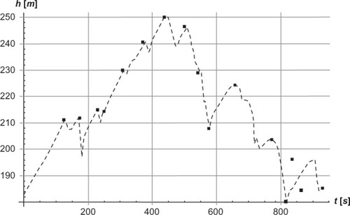
The Diff shows that the power balance model with varying work rate P fits better on uphill compared to downhill terrain. From 0 seconds to 437 seconds (mostly uphill terrain), the Diff equals 10, while during the downhill terrain the Diff equals 115.

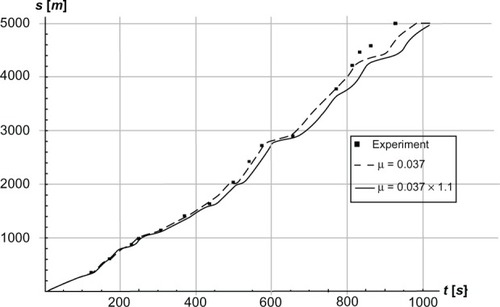
When increasing the friction coefficient by 10%, from 0.037 to 0.037 × 1.1, the skier is delayed around 200 m after 5 km (Figure 7). This is roughly 200 m/5000 m = 4%, which is comparable to a 4% increase in time (for simplicity, assuming average speed and incline for the last 200 m).

Figure 7 Simulated and experimental positions s in meters as a function of time t in seconds along the track while skiing on snow using the skating technique.

Notes: P = 253 Joules per second (J/s) on uphill sections and P = 197 J/s on downhill sections. Dashed line: μ = 0.037; Solid line: μ = 0.037 × 1.1; ■: Experimental values.

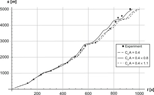
With a 10% larger air drag coefficient, the skier is delayed by around 3% (Figure 8). Also, a case where the air drag coefficient was reduced by 20% was simulated, in which the skier was around 5% faster.

Figure 8 Simulated and experimental positions s in meters as a function of time t in seconds along the track while skiing on snow using the skating technique. P = 253 Joules per second (J/s) on uphill sections and P = 197 J/s on downhill sections.

Notes: Long-dashed line: C_dA = 0.4; Dashed line: C_dA = 0.4 1.1; Solid line: C_dA = 0.4 × 0.8; ■: experimental values.

Discussion

The literature measures work rate in skiing repeatedly on treadmills, but has not previously provided a model that predicts how the work rate P evolves during actual skiing. The common approach in physiology and biomechanics is to look backwards in time. In this paper, we looked into the future and determined the work rate P by applying the hypothetical inductive deductive method (predicting the skier’s position during competition thus corresponds to predicting planetary movement in astronomy).

Previously, Carlsson et al¹⁶ have analyzed the resistant forces caused by gravity, ski friction, and air drag interacting with locomotive forces caused by the skier. We extended this research by comparing the current simulations with actual skiing on snow, which showed that the power balance model was useful for analyzing how various factors influence cross-country skiing performance. Simulated and actual positions had the best fit on uphill terrain, where the model seems to be particularly good. This may be influenced by all measurements conducted on the treadmill that were performed uphill. Thus, to improve the model, future research should conduct downhill treadmill measurements with different speeds and inclinations, and analyze the transitions between uphill and downhill terrain.

The experimental points 14–16 differed more than expected from the simulation, which might be caused by the curved terrain that is difficult to simulate in these sections. Additionally, some of the differences between the experimental and simulated positions here may have been caused by an inaccurate map in this constantly varying and curved terrain. When we checked the location of these points on the map with a GPS post-test, this test indicated that points 14 and 15 differed slightly from the map. In future studies we suggest that more accurate measurements of rapidly changing terrain is required to ensure that the map is correct.

This paper’s model provides a tool that clarifies how multiple factors interact to influence a skier’s speed at various points during skiing. This tool may help skiers to better prioritize training in order to reach the finish line in minimum time. Essential in the model is Newton’s second law for a skier in Equation 18$\begin{array}{l}m\frac{dv}{dt}=P/v(t)-mgSin\left(\alpha (s(t))\right)-mg\mu Cos\left(\alpha (s(t))\right)-\frac{1}{2}\rho C_{d}Av{(t)}^2,\hfill \\ \frac{ds}{dt}=v(t),\hfill \end{array}$(18) , which gives the equation of motion of the skier’s center of mass, and specifies the relations between speed v, time t, work rate P, angle of inclination α, and a variety of characteristics. Understanding Equation 18$\begin{array}{l}m\frac{dv}{dt}=P/v(t)-mgSin\left(\alpha (s(t))\right)-mg\mu Cos\left(\alpha (s(t))\right)-\frac{1}{2}\rho C_{d}Av{(t)}^2,\hfill \\ \frac{ds}{dt}=v(t),\hfill \end{array}$(18) enables a skier to train optimally to win races. Solving Equation 18$\begin{array}{l}m\frac{dv}{dt}=P/v(t)-mgSin\left(\alpha (s(t))\right)-mg\mu Cos\left(\alpha (s(t))\right)-\frac{1}{2}\rho C_{d}Av{(t)}^2,\hfill \\ \frac{ds}{dt}=v(t),\hfill \end{array}$(18) presupposes that the role of the work rate P is determined, which demonstrates that skiers with the largest work rate P are not necessarily the fastest. For example, heavy skiers may have a high work rate P uphill, but due to the greater resistant forces from gravity on this terrain they may have lower speeds than smaller skiers with a lower work rate P. More generally, skiers with different body mass, drag areas, friction coefficients, and so on, but with the same work rate P, will have different speeds and positions as a function of time.

As an aid to determine the work rate P, we tested four models of metabolic rate, referred to as Q, Q_A, Q_B, and Q_C, against experimental data on the treadmill. The four models showed the linkages between metabolic rate, heart rate, VO₂(t), VCO₂(t), and work rate in steady state and dynamic situations. The steady state model dQ_C(t)/dt = 0 and dynamic model Q used the work rate P as determined by the power balance equation as input. The model Q_A rate of oxygen consumption and rate of carbon dioxide production as input. The model Q_B used heart rate and rate of carbon dioxide production as input. One problem when using heart rate measurements to determine metabolic rate is that these values may drift upwards up to 20% during skiing (possibly due to body heat) despite VO₂(t) being constant. Such a drift in heart rate does not reflect the VO₂(t) influences on a skier’s speed (for example, a very high heart rate usually causes lower speed); however, altogether the data suggest that heart rate is a reasonable measure of metabolic rate during cross-country skiing on varying terrain.

We tested Equation 18$\begin{array}{l}m\frac{dv}{dt}=P/v(t)-mgSin\left(\alpha (s(t))\right)-mg\mu Cos\left(\alpha (s(t))\right)-\frac{1}{2}\rho C_{d}Av{(t)}^2,\hfill \\ \frac{ds}{dt}=v(t),\hfill \end{array}$(18) with two assumptions for work rate P: first, that it is constant; and second, that the value is larger uphill than downhill. Our heart rate measurements supported that the work rate P downhill compared to uphill is 70/90. The 70/90 finding expands upon findings from earlier studies that have not sufficiently quantified how uphill work rates are higher than work rates on level or downhill terrain during competitions.^4,18 In the current study, this could be explained by two main factors: (1) the skier was unable to ski at the same metabolic rate on downhill compared to uphill terrain, as shown previously by Mognoni et al;⁹ and (2) the skier had a reduced ability to produce work when speed increased on downhill terrain. Sandbakk et al¹⁹ found that the differences in the skier’s ability to produce work rate (as defined above) while ski skating on different inclines reflects alterations in the technique employed by the skier at different speeds. Furthermore, the skier had a higher gross efficiency (ie, work rate divided by metabolic rate) on steeper uphill inclines, as was found earlier both in skiing and other exercise modes.^19,23,30

In the simulation model with the second assumption of varying work rates P, the effects of friction and air drag on total skiing time were calculated. These analyses indicated that there was a 4% and 3% improved skiing performance by 10% reduced friction or air drag coefficients, respectively. Changes in friction or drag as much as 10% are probably only possible in extreme scenarios but in most international races in cross-country skiing, time differences of less than 1% to complete the race separates a first- and fourth-place skier (http://www.fis-ski.com). Thus, optimizing these factors may determine whether an athlete wins a medal or not in cross-country skiing.

To further improve the current simulation model, more data on how work rate, metabolic rate, and efficiency changes across the different skating techniques, speeds, and inclines would be advantageous. Within these techniques, more accurate measures of work against friction and air drag would be a future objective for improving the model. Here, the effects of the constantly varying normal force during a cycle on the friction coefficient should be further analyzed. Also, the impact of using poles for propulsion on normal forces and work against friction, as well as the effects of angling and edging the skis while skating on the friction coefficient, are missing in the current model. Regarding air drag, different projected front area for the skier as a function of skating technique should be considered, and the different skating techniques should be analyzed in their specific dynamic movements rather than including data from static positions, such as in the current model. Also, cycle rate may affect the metabolic cost of unloaded skiing (ie, zero work rate) and should be incorporated in the calculations. Finally, the drift in heart rate should be considered when heart rate data is used to assess metabolic rate; also of interest for further development of the model is the establishment of a generic model on how the skier changes the work rate P on uphill and downhill terrain.

In conclusion, the power balance model was found to be a useful tool for analyzing how various factors influence performance in cross-country skiing on varying terrain. A skier’s position along the track was simulated reasonably well when compared to experimental data while skiing on snow, with the best fit observed when the work rate was increased on uphill and reduced on downhill terrain. The model predicted that the skiing time increased by 3%–4% when friction or air drag increased by 10%. Future research can assess the power balance model for different skiers with different proficiency levels, fitness levels, height, age, and sex to determine how different skiers’ characteristics influence their abilities to reach the finish line in minimum time.

Acknowledgments

We thank three anonymous reviewers of this manuscript, as well as Felix Breitschädel for his useful comments. We thank Hermod Bjørkestøl, the International Ski Federation officer who is responsible for homologations, for informing us on how tracks are designed and measured.

Supplementary materials

A. Estimating the parameters c₁, c₂ and c₃ for λ(α)

Our data set could not uniquely determine λ(α) by a least squares fit to the data. Thus, λ(α) was determined using a two-step procedure. The two-step procedure is analogous to a root-finding algorithm for finding a value x so that f(x) = 0. The first step is an initial guess of a value of x, or a range within which x falls. The second step consists of iteration, where x hopefully approaches a limit referred to as a fixed point or root. For our purpose, we first chose three points on the λ(α) function expressed with the list

${\lambda }_L=\left\{\right\{0.02,{\lambda }_1\},\{0.05,1\},\{0.12,{\lambda }_2\left\}\right\},$(S1)

where 0.02, 0.05, and 0.12 are three angles of inclination expressed in radians. The values of the function

${\lambda }_{*}=(\alpha ,{\lambda }_1,{\lambda }_2)=c_{*1}({\lambda }_1,{\lambda }_2)\left(1+c_{*1}({\lambda }_1,{\lambda }_2)(Exp\left(-c_{*3}({\lambda }_1,{\lambda }_2)\alpha \right)\right)$(S2)

were fitted to this list by a least squares fit for each chosen pair, (λ₁, λ₂). Visual curve fitting means choosing plausible values for λ₁ and λ₂, plotting the metabolic rate

$Q_{*}=Q_0+Q_1^{0.05}(P)\cdot {\lambda }_{*}(\alpha ,{\lambda }_1,{\lambda }_2),$(S3)

and comparing these values visually with the experimental data for the three angles. The values of λ₁ and λ₂ were changed repeatedly until a good visual fit was obtained, while ensuring that λ₁ and λ₂ have physiological trustworthy numerical values. Second, a least squares fit to the data was performed to produce ex post best fit estimates of λ₁ and λ₂ using the visual estimates as starting guess points, and choosing a range around each starting point for λ₁ and λ₂. The method was performed separately for each parameter λ₁ and λ₂, keeping the other parameter fixed. We refer to

$\begin{array}{l}{Q}_{*}=Q_0+Q_1^{0.05}(P)\cdot {\lambda }_{*}(\alpha ,{\lambda }_1,{\lambda }_2)\hfill \\ \text{as\hspace{0.17em}}{Q}_{*}(P,\alpha ,{\lambda }_i),i=1,2,\hfill \end{array}$(S4)

which is the metabolic rate dependent on λ_i for one of the two parameters. The expression Q_*(P,α,λ_i) – Q_d(P,α) is the difference between Q_* and the experimentally determined Q_d(P,α) at work rate P and the angle of inclination α. The root of the square difference summed over the discrete data points is

$Diff({\lambda }_i)={\left({\displaystyle {\sum }_j{\left(Q_{*}\left(P_j,{\alpha }_j,{\lambda }_i\right)-Q_d\left(P_j,{\alpha }_j\right)\right)}^2}\right)}^{1/2},$(S5)

where P_j and α_j are the discrete work rates and angles where we have data points.

Steps 1 and 2 were repeated many times until we were certain that we had obtained the optimal values for λ_1opt and λ_2opt, which gives the minimum Diff for each of the two parameters. Thereafter we chose

$\lambda (\alpha )={\lambda }_{*}(\alpha ,{\lambda }_{1opt},{\lambda }_{2opt})$(S6)

and found

${\lambda }_{1opt}=1.17,{\lambda }_{2opt}=0.92,$(S7)

and

$c_1=c_{*1}\left({\lambda }_{1opt},{\lambda }_{2opt}\right)=0.91,c_2=c_{*2}\left({\lambda }_{1opt},{\lambda }_{2opt}\right)=0.62,c_3=c_{*3}\left({\lambda }_{1opt},{\lambda }_{2opt}\right)=37.59$(S8)

B. Measuring distances along the track, and associated uncertainties

The track profile was made by the Norwegian Ski Federation according to the recommendations for World Cup races using a measuring wheel and a global positional system (GPS). For this study, we also checked the track distance by a GPS Garmin eTrex10 (Garmin International, Inc, Olatha, Kansas, USA) with Wide Area Augmentation System receivers, which has an accuracy of less than 3 m horizontally and vertically with the current satellite availability. Using the GPS watch on a running track revealed around 1–2 m of incorrectness per km. During the summer, the track in the terrain was measured to be 4996 m by GPS. Tracks for international skiing competitions are made during the summertime with the help of local authorities by designing a map at scale 1:2000 and contour intervals of 1 m. The track was plotted onto the map and a three-dimensional terrain model resulting in a digitized map was designed, providing a track profile with all terrain details. The terrain may be adjusted to create a good track with nice turns (for example, to provide skiing pleasure, or to prevent accidents). Distance and height along the track are measured using a measuring wheel and an inclinometer (Suunto Oy, Vantaa, Finland). Points of measurement are usually where the elevation changes 10–20 meters vertically. Horizontal measurements depend on how successfully the skier follows the ideal track. For mass start races, the track is the same as the ideal track. For interval starts, the length is usually determined by the inner turn in each curve. The common measurement method is to take the required track data from the digitized map. These data, rounded to the closest integer meter, are inserted into the computer program developed by the International Ski Federation in order to provide the required documentation.

C. Simulations fit with the experimental data

To check how well the simulations fit the experimental data, we calculated the root mean square time difference Diff between the skier and the simulated skier’s time (t) at different positions. We defined

$\begin{array}{r}\hfill Diff=\sqrt{{\displaystyle \sum _{i=1}^z\text{Δ}{t}_i^2}},\text{\hspace{0.17em}Δ}{t}_i=t_i-t\left(s_{\exp }(t_i)\right),\\ \hfill s=s(t)\Rightarrow t=t(s),\text{\hspace{0.17em}with\hspace{0.17em}}{s}_{exp}(t_i)\end{array}$(S9)

as the experimental position as a function of time (t_i), and 16 is the number of times these measurements were performed. In addition, s(t_i) is the simulated position at t_i. We found it methodologically beneficial to solve the differential equation in Equation 18$\begin{array}{l}m\frac{dv}{dt}=P/v(t)-mgSin\left(\alpha (s(t))\right)-mg\mu Cos\left(\alpha (s(t))\right)-\frac{1}{2}\rho C_{d}Av{(t)}^2,\hfill \\ \frac{ds}{dt}=v(t),\hfill \end{array}$(18) for the inverse function by solving t’(s) = 1/s’(t(s)), where the apostrophe indicates the derivative with respect to t(s). The reason for this is that it is mathematically easier to solve this simple ordinary differential equation than solving the algebraic equation s(t) = t_i to find the time t for every experimental t_i.

Disclosure

The authors report no conflicts of interest in this work.