The development of an affinity evaluation and prediction system by using protein–protein docking simulations and parameter tuning

Abstract

A system was developed to evaluate and predict the interaction between protein pairs by using the widely used shape complementarity search method as the algorithm for docking simulations between the proteins. We used this system, which we call the affinity evaluation and prediction (AEP) system, to evaluate the interaction between 20 protein pairs. The system first executes a “round robin” shape complementarity search of the target protein group, and evaluates the interaction between the complex structures obtained by the search. These complex structures are selected by using a statistical procedure that we developed called ‘grouping’. At a prevalence of 5.0%, our AEP system predicted protein–protein interactions with a 50.0% recall, 55.6% precision, 95.5% accuracy, and an F-measure of 0.526. By optimizing the grouping process, our AEP system successfully predicted 10 protein pairs (among 20 pairs) that were biologically relevant combinations. Our ultimate goal is to construct an affinity database that will provide cell biologists and drug designers with crucial information obtained using our AEP system.

Keywords:

• protein-protein interaction
• affinity analysis
• protein-protein docking
• FFT
• massive parallel computing

Introduction

Proteins have diverse functions ranging from molecular machines to signaling. They participate in catalytic reactions, provide transport, form viral capsids, traverse membranes and construct regulated channels, transmit information from DNA to RNA, thus making it possible to synthesize new proteins. Given their importance, considerable effort has centered on the prediction of protein functions. A major way of achieving this is through the identification of binding partners. If we know the function of at least one of the components with which the protein interacts, that should enable us to determine its function(s) and the pathway(s) in which it plays a role. This holds since the vast majority of the functions performed by proteins in living cells involve protein–protein interactions (PPI).^1,2 Hence, by observing the intricate network of these interactions we can map cellular pathways, their interconnectivities and their dynamic regulation. Their identification is at the heart of functional genomics; their prediction is crucial to the discovery of new drugs. Knowledge of these pathways, their topologies, lengths, and dynamics may provide useful information for forecasting side effects.

The PPI affinity problem involves finding a protein pair that is interactive from a protein group with a known structure.^1,2 Recently, pharmaceutical companies have been trying to produce medicines based on candidates discovered using protein– chemical compound docking simulations. Docking analysis with respect to PPI remains limited, however, because the macromolecules involved in these simulations are large and thus require extensive computational resources. PPI is a basic element of model construction in research that first analyzes the cell-signaling pathway and then identifies the target protein of a drug. The prediction of the interactions between vast numbers of proteins is crucial if we are to understand such biological phenomena as cellular signaling, enzyme reaction and gene expression regulation.

PPI prediction has been extensively studied both experimentally^3–7 and theoretically. In experimental studies, Giot and colleagues,⁸ and Stanyon and colleagues⁹ constructed a protein interaction map on a genome scale for Drosophila melanogaster, and Rain and colleagues¹⁰ constructed that for human Helicobacter pylori. Based on theoretical calculations, Wojcik and colleagues¹¹ constructed an interaction map by using domain profile pairs in which the input was the amino acid sequence for H. pylori.

These studies mainly used either genome scale analysis^8,10 or sequence analysis.¹² However, in vivo, PPI is achieved by using protein structural information. Therefore, ultimately, PPI evaluation and prediction should also utilize protein structural information. Such an interaction evaluation and prediction system has been discussed by Smith and colleagues,¹³ they did not consider the composition, performance or accuracy of the evaluation or the prediction of a concrete system. If we can perform such an ultimate PPI evaluation and prediction of the interaction between pairs of a large number of proteins, we can assume a signal transmission pathway, and then we can evaluate and predict the affinity between an enzyme and inhibitor(s) or substrate(s), an antibody and an antigen. Such a large-scale PPI affinity evaluation system has been discussed by Park and colleagues¹⁴ and Gong and colleagues.¹⁵ Their system, Protein Structural Interactome map (PSIMAP) (http://psimap.com/), performs evaluations by using Euclidean distance between two domains and the number of residue pairs within a given distance threshold as the PPI measurement base. This method is simple and fast. We know that the data provided by PSIMAP are useful, but such a method based on simply distance comparisons is not available for making PPI maps that include sufficient three-dimensional (3D) structural information for supporting a drug discovery. Therefore, in this study we developed a high-speed and more detailed PPI affinity evaluation and prediction system that is based on our original docking simulation program and the original high-speed FFT library produced by Hourai and colleagues¹⁶ and can be performed using a massive parallel PC cluster. In this system, which we call an affinity evaluation and prediction (AEP) system, first a “round robin” shape complementarity search is executed for the target protein group, and then the interaction between the proteins is evaluated based on complex structures determined by using a statistical procedure that we developed called ‘grouping’.

Methods

Evaluation of shape complementarity

When the shape complementarity^17–19 between two proteins is evaluated, the structure of a protein is converted into a rigid body object represented in a 3D grid space. Typically, in the protein–protein docking simulation, each point of the protein represented on the grid is classified as being in the core area, the surface area, or the cavity area as described below. Because the accuracy of docking simulations that use the shape complementarity search depends strongly on the representation method, various representation methods have been developed.

Here, we have developed a representation method called the voxel model, which has two distinguishing features. (1) The molecular surface can be faithfully modeled by changing the radius of the probe sphere to define as the extended solvent-accessible surface, which is traced out by the probe sphere center as it rolls over the protein, of each atomic type. (2) The shape complementarity can be determined much more accurately than just made voxel models by reducing the thickness of the molecular surface. However, when the thickness is reduced too much, the response of the shape complementarity evaluation function becomes too sensitive. Next we describe in detail the voxel model and the procedure for converting the crystal structure of a protein to the voxel model (voxelization).

Voxelization

The voxel model is expressed as shown in expression (1$\begin{array}{l}\mathit{\nu }=\{I,O,S,C\mid I\cap O\cap S\cap C=\phi \}\\ I=\{I_i\mid i\in \mathbf{N},0\le i\le n_I\}\\ O=\{O_j\mid j\in \mathbf{N},0\le j\le n_O\}\\ S=\{S_k\mid k\in \mathbf{N},0\le k\le n_S\}\\ C=\{C_I\mid l\in \mathbf{N},0\le l\le n_C\}\\ 0\le n_I,n_O,n_S,n_C\le n_V\mid n_V\in \mathbf{N},n_V\ge 0\\ 0\le n_I+n_O+n_S+n_C\le n_V\mid n_V\in \mathbf{N},n_V\ge 0\end{array}$(1) ), where VOXEL (V) represents the voxel model, INNER (I) defines the area on the atom, where the protein exists, OUTER (O) is the area that is not INNER, in other words it indicates a solvent. SURFACE (S) is the area on the molecular surface of the protein, CAVITY (C) is the area inside SURFACE that is not INNER, namely, it means a cavity. N is a set of natural numbers, and φ is an empty set. n_I, n_O, n_S, and n_C are the upper bound values of each voxel type (I, O, S, C) decided from the molecular size of the protein. All the areas in the voxel space in the initial state are defined as DEFAULT (D), and a temporary molecular surface of protein is defined as TMP_SURFACE (S_tmp).

$\begin{array}{l}\mathit{\nu }=\{I,O,S,C\mid I\cap O\cap S\cap C=\phi \}\\ I=\{I_i\mid i\in \mathbf{N},0\le i\le n_I\}\\ O=\{O_j\mid j\in \mathbf{N},0\le j\le n_O\}\\ S=\{S_k\mid k\in \mathbf{N},0\le k\le n_S\}\\ C=\{C_I\mid l\in \mathbf{N},0\le l\le n_C\}\\ 0\le n_I,n_O,n_S,n_C\le n_V\mid n_V\in \mathbf{N},n_V\ge 0\\ 0\le n_I+n_O+n_S+n_C\le n_V\mid n_V\in \mathbf{N},n_V\ge 0\end{array}$(1)

The procedure of voxelization is formulated using expression (2$\begin{array}{l}\mathit{\nu }=(step\hspace{0.17em}1)\to \{D\}-(step\hspace{0.17em}2)\to \{I,D\}-(step\hspace{0.17em}3)\\ \to \{I,O,D\}-(step\hspace{0.17em}4)\to \{I,O,S_{tmp},D\}-(step\hspace{0.17em}5)\\ \to \{I,O,S,D\}-(step\hspace{0.17em}6)\to \{I,O,S,C\}\end{array}$(2) ). Figure 1 details each step of this procedure.

Figure 1 Six-step voxelization process for the quantization and characterization of protein surfaces in our AEP system.

Abbreviation: AEP, affinity evaluation and prediction.

$\begin{array}{l}\mathit{\nu }=(step\hspace{0.17em}1)\to \{D\}-(step\hspace{0.17em}2)\to \{I,D\}-(step\hspace{0.17em}3)\\ \to \{I,O,D\}-(step\hspace{0.17em}4)\to \{I,O,S_{tmp},D\}-(step\hspace{0.17em}5)\\ \to \{I,O,S,D\}-(step\hspace{0.17em}6)\to \{I,O,S,C\}\end{array}$(2)

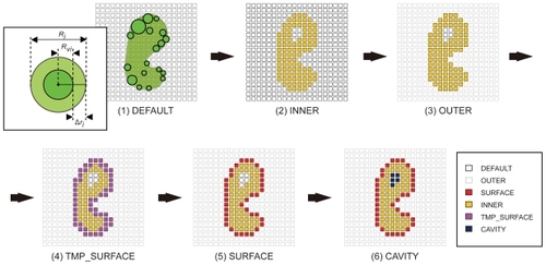
• Step 1 (DEFAULT):

  In the voxel space, all grid points are assigned to DEFAULT as the initial state.

• Step 2 (INNER):

  The grid points that exist within a spheroid of radius R_i (=R_viΔr_i) are assigned to INNER, where R_vi is the van der Waals radius of each atom, and Δr_i is the increment in the radius of a defined type of atom.

• Step 3 (OUTER):

  All the remaining grid points are assigned as OUTER.

• Step 4 (TMP_SURFACE):

  The INNER grid points that adjoin the OUTER grid points are newly assigned to TMP_SURFACE.

• Step 5 (SURFACE):

  A TMP_SURFACE grid point is finally replaced by SURFACE or INNER according to the following process. When a TMP_SURFACE grid point is enclosed by six or more OUTER grid points, the TMP_SURFACE grid point is re-assigned to SURFACE. After this process has been completed for all TMP_SURFACE grid points, the remaining TMP_SURFACE grid points are re-assigned to INNER. Thus, finally, the TMP_SURFACE grid points vanish from the voxel space.

• Step 6 (CAVITY):

  The grid points which remain as DEFAULT are re-assigned to CAVITY. Hence, the DEFAULT grid points also disappear from the voxel space.

Score function of contact surface area

In the shape complementarity evaluation, the surface contact between proteins represented by the grid points is evaluated by using the score function of the contact surface area.¹⁷ This score function defines a score for INNER, OUTER, SURFACE, and CAVITY as described in Voxelization. The contact surface score function we adopted for our voxel model is the pair-wise shape complementarity (PSC) score function S_PSC that Weng and colleagues¹⁷ defined with ZDOCK.^17,18,20 As defined in expressions (3$\begin{array}{l}\text{Re}[R_{PSC}(l,m,n)]\\ =\{\begin{array}{ll}\begin{array}{l}number\hspace{0.17em}of\hspace{0.17em}SURFACE\hspace{0.17em}within\\ (vdw\hspace{0.17em}radius\hspace{0.17em}of\hspace{0.17em}Carbon+bonusR)\end{array}\hfill & OUTER\hfill \\ 0\hfill & otherwise\hfill \end{array}\\ \text{Re}[L_{PSC}(l,m,n)]\\ =\{\begin{array}{ll}1\hfill & SURFACE,INNER\hfill \\ 0\hfill & otherwise\hfill \end{array}\\ \text{Im}[R_{PSC}(l,m,n)]=\text{Im}[L_{PSC}(l,m,n)]\\ =\{\begin{array}{ll}3\hfill & SURFACE\hfill \\ 9\hfill & INNER,CAVITY\hfill \\ 0\hfill & OUTER\hfill \end{array}\end{array}$(3) ) and (4$\begin{array}{l}{S}_{PSC}(o,p,q)\\ =\text{Re}\left[\sum _{l=1}^N\sum _{m=1}^N\sum _{n=1}^N{R}_{PSC}(l,m,n)·L_{PSC}(l+o,m+p,n+q)\right]\\ =\text{Re}\left[\frac{1}{N^3}IFT(IFT(R_{PSC})·DFT(L_{PSC}))\right]\\ -\text{Im}\left[\frac{1}{N^3}IFT(IFT(R_{PSC})·DFT(L_{PSC}))\right]\end{array}$(4) ), this S_PSC is a primitive function where the electrostatic interaction is not considered. The score function S_PSC consists of two factors R_PSC, L_PSC.

$\begin{array}{l}\text{Re}[R_{PSC}(l,m,n)]\\ =\{\begin{array}{ll}\begin{array}{l}number\hspace{0.17em}of\hspace{0.17em}SURFACE\hspace{0.17em}within\\ (vdw\hspace{0.17em}radius\hspace{0.17em}of\hspace{0.17em}Carbon+bonusR)\end{array}\hfill & OUTER\hfill \\ 0\hfill & otherwise\hfill \end{array}\\ \text{Re}[L_{PSC}(l,m,n)]\\ =\{\begin{array}{ll}1\hfill & SURFACE,INNER\hfill \\ 0\hfill & otherwise\hfill \end{array}\\ \text{Im}[R_{PSC}(l,m,n)]=\text{Im}[L_{PSC}(l,m,n)]\\ =\{\begin{array}{ll}3\hfill & SURFACE\hfill \\ 9\hfill & INNER,CAVITY\hfill \\ 0\hfill & OUTER\hfill \end{array}\end{array}$(3)

The factor R_PSC(l, m, n) is for the receptor protein, which is a protein fixed on the grid space, and the factor L_PSC(l, m, n) is for the probe protein, which is a protein that is rotated and translated on the grid space. In expressions (3$\begin{array}{l}\text{Re}[R_{PSC}(l,m,n)]\\ =\{\begin{array}{ll}\begin{array}{l}number\hspace{0.17em}of\hspace{0.17em}SURFACE\hspace{0.17em}within\\ (vdw\hspace{0.17em}radius\hspace{0.17em}of\hspace{0.17em}Carbon+bonusR)\end{array}\hfill & OUTER\hfill \\ 0\hfill & otherwise\hfill \end{array}\\ \text{Re}[L_{PSC}(l,m,n)]\\ =\{\begin{array}{ll}1\hfill & SURFACE,INNER\hfill \\ 0\hfill & otherwise\hfill \end{array}\\ \text{Im}[R_{PSC}(l,m,n)]=\text{Im}[L_{PSC}(l,m,n)]\\ =\{\begin{array}{ll}3\hfill & SURFACE\hfill \\ 9\hfill & INNER,CAVITY\hfill \\ 0\hfill & OUTER\hfill \end{array}\end{array}$(3) ) and (4$\begin{array}{l}{S}_{PSC}(o,p,q)\\ =\text{Re}\left[\sum _{l=1}^N\sum _{m=1}^N\sum _{n=1}^N{R}_{PSC}(l,m,n)·L_{PSC}(l+o,m+p,n+q)\right]\\ =\text{Re}\left[\frac{1}{N^3}IFT(IFT(R_{PSC})·DFT(L_{PSC}))\right]\\ -\text{Im}\left[\frac{1}{N^3}IFT(IFT(R_{PSC})·DFT(L_{PSC}))\right]\end{array}$(4) ), l, m, and n are the coordinates of the grid point, and “Re[]” and “Im[]”, respectively, indicate the real and imaginary parts of the factor and the PSC scoring function. Moreover, bonusR, which appears in the real part of R_PSC(l, m, n), indicates “bonus” points (ie, additional points added to the PSC scoring) when the probe protein penetrates the pocket structure of the receptor protein. The final S_PSC, as shown by expression (4$\begin{array}{l}{S}_{PSC}(o,p,q)\\ =\text{Re}\left[\sum _{l=1}^N\sum _{m=1}^N\sum _{n=1}^N{R}_{PSC}(l,m,n)·L_{PSC}(l+o,m+p,n+q)\right]\\ =\text{Re}\left[\frac{1}{N^3}IFT(IFT(R_{PSC})·DFT(L_{PSC}))\right]\\ -\text{Im}\left[\frac{1}{N^3}IFT(IFT(R_{PSC})·DFT(L_{PSC}))\right]\end{array}$(4) ), is obtained by calculating the correlation function between R_PSC and L_PSC. The computational complexity of this calculation is O(N⁶), but can be decreased to O(N³logN) by using a fast Fourier transform (FFT) as follows.

$\begin{array}{l}{S}_{PSC}(o,p,q)\\ =\text{Re}\left[\sum _{l=1}^N\sum _{m=1}^N\sum _{n=1}^N{R}_{PSC}(l,m,n)·L_{PSC}(l+o,m+p,n+q)\right]\\ =\text{Re}\left[\frac{1}{N^3}IFT(IFT(R_{PSC})·DFT(L_{PSC}))\right]\\ -\text{Im}\left[\frac{1}{N^3}IFT(IFT(R_{PSC})·DFT(L_{PSC}))\right]\end{array}$(4)

Abbreviations: (DFT, Discrete Fourier Transform; IFT, Inverse Fourier transform).

In the S_PSC calculation, we adopted the FFT library CONV3D developed by Hourai and Nukada.¹⁶ The CONV3D is highly optimized for specific CPU architectures (Pentium, Xeon, Athlon, POWER5, etc.), achieves high-speed performance, and is about three times faster than the widely used FFT library package FFTW^21,22 (according to the results obtained with Protein–Protein Docking Benchmark 2.0;²³ data not shown).

At the beginning, a rotational search is performed in an actual evaluation of the contact surface between proteins. The rotational search works by explicitly rotating the ligand protein around each of its three Cartesian angles by a certain increment (15 degrees in this study). A total of 3600 rotated bodies of the ligand protein are thus generated. Next, the shape complementarity evaluation is undertaken for all rotated bodies. If the grid size of the ligand protein is N³, then N³ × 3600 PSC scores must be calculated. Based on preliminary experiments, in all the analyses we only extracted the top-ranked 512 PSC scores for the following procedures.

Reliability of shape complementarity evaluation

To confirm the reliability of the shape complementarity evaluation by using our voxel model, we performed simple docking calculations using some bound structures adopted from Weng’s Protein–Protein Docking Benchmark 2.0 as samples. It is widely recognized that the main challenge in protein docking lies in the unbound–bound transition. Although we are also more interested in the unbound experiments than in the bound, the latter enables us to primitively confirm the advantages of our AEP’s improvement at the initial stage. Because a protein complex for the latter, which is pulled apart and reassembled, is more complementary than individually crystallized component structures for the former. The widely used i-RMSD (backbone RMSD at the interface) was the criterion we used to evaluate the reliability. In this way we evaluated the difference between the complex structure obtained by using the docking calculation and the X-ray crystal structure.

Affinity analysis

To calculate protein-protein affinity, we assess the biological relevance of target proteins by statistically analyzing the characteristics of shape complementarity. The affinity analysis involved processing the 512 top-ranked values of S_PSC obtained from the shape complementarity evaluation by using a clustering method that we call grouping. The following describes the affinity prediction procedure and includes a description of the grouping method.

• Step 1 (Shape complementarity evaluation):

  A shape complementarity evaluation of protein pairs is performed. Only the 512 top-ranked S_PSC scores are then considered for step 2.

• Step 2 (Grouping):

  The purpose of step 2 is to classify the 512 S_PSC scores into 10 clusters, C_i (i = 1–10). First, the clustering method is performed hierarchically by using the nearest neighbor method for the 512 values of S_PSC as follows. We define the targeted dataset X = {x₁, ..., x₅₁₂} as consisting of 512 S_PSC scores from step 1. For each data point, x_i is represented as x_i = (S_i, T_i(T_X, T_Y, T_Z), R_i(R_θ, R_φ, R_ψ)). Here, S_i = S_PSC from expression (4$\begin{array}{l}{S}_{PSC}(o,p,q)\\ =\text{Re}\left[\sum _{l=1}^N\sum _{m=1}^N\sum _{n=1}^N{R}_{PSC}(l,m,n)·L_{PSC}(l+o,m+p,n+q)\right]\\ =\text{Re}\left[\frac{1}{N^3}IFT(IFT(R_{PSC})·DFT(L_{PSC}))\right]\\ -\text{Im}\left[\frac{1}{N^3}IFT(IFT(R_{PSC})·DFT(L_{PSC}))\right]\end{array}$(4) ), T_i(T_X, T_Y, T_Z) is the amount of translation for the ligand protein in the grid space, and R_i(R_θ, R_φ, R_ψ) is a rotation parameter for the ligand protein. If (o,p,q) in expression (4$\begin{array}{l}{S}_{PSC}(o,p,q)\\ =\text{Re}\left[\sum _{l=1}^N\sum _{m=1}^N\sum _{n=1}^N{R}_{PSC}(l,m,n)·L_{PSC}(l+o,m+p,n+q)\right]\\ =\text{Re}\left[\frac{1}{N^3}IFT(IFT(R_{PSC})·DFT(L_{PSC}))\right]\\ -\text{Im}\left[\frac{1}{N^3}IFT(IFT(R_{PSC})·DFT(L_{PSC}))\right]\end{array}$(4) ) is used, then o = T_X, p = T_Y, and q = T_Z in T_i(T_X, T_Y, T_Z), respectively.

  All data x belonging to the dataset X are sorted by the rank order of S_i. In X, we define the data point with the maximum S_i (maxS_i) as the central data y₁ of cluster 1 (y₁ ∈C₁). Here, the term central data indicates data that represent a characteristic of a cluster. Now, we introduce the distances D₁(y₁, x_i) and D₂(y₁, x_i) between y₁ and x. Here, in this dataset x, the data y₁ is not included and is not classified into any clusters C_i (x_i ∈ (C_i)^C). The distance D₁ is represented as the Euclidean translation distance, and the rotational distance D₂ is a value defined to represent the difference in rotation of data x_i and data y₁. Here, we define the center of gravity of a ligand as point G and the coordinates of the C_α atom in the C- and N-terminals of a ligand as points C and N, respectively. We also define vector u as the normal vector of a plane, which is defined by three points (G, C, and N). Thus, the rotational difference D₂ indicates the cosine between u_i of data x_i and u₁ of data y₁. When the following two conditions exist between the above data x_i (ie, x_i ∈ (C_i)^C) and the central data y₁, the data x_i are classified into cluster 1 (C₁).

  1. When the translation distance |D₁| between T_i of data x_i and T₁ of the central data y₁ is less than a certain translational threshold (eg, 10.0Å).

  2. When the rotational distance |D₂| between x_i and y₁ is less than a certain rotational threshold (eg, π/6).

     Cluster C₁ is determined by repeating step 2 for all x_i where y₁ is excluded. Similarly, step 2 is repeated for clusters C_i (i = 2–10). Step 2 ends either when the ten clusters (C₁–C₁₀) are generated or when all x_i belong to any cluster C_i.

• Step 3 (Calculation of Z-score):

  The purpose of step 3 is to prepare for the affinity analysis. The Z-score indicates the number of standard deviations that an observation is above or below the mean. It allows us to compare observations from different normal distributions. Here, a set of central data y_i of each cluster C_i obtained in step 2 is defined as the central dataset Y. The distribution Z_score(y_i) is the Z-score distribution of the PSC score of each set of central data y_i ∈ Y when the dataset X is considered a population. The distribution Z_conformation(C_i) is the distribution of the Z-score of m_Ci. Here m_Ci is the number of data that constitute cluster C_i when the dataset M_cluster = {m_ci | i ∈ N, i ≧0} is considered a population. In step 3, the distributions Z_score(y_i) and Z_conformation(C_i) are calculated.

• Step 4 (Calculation of affinity score S_affinity):

  The measure for the affinity analysis is called an affinity score S_affinity, which is defined in expression (5$\begin{array}{l}{S}_{affinity}=\text{max}(w_s·Z_{score}(y_i)+w_C·Z_{conformation}(C_i))\\ w_s:weighting\hspace{0.17em}factor\hspace{0.17em}for\hspace{0.17em}{Z}_{score}(y_i)\\ w_e:weighting\hspace{0.17em}factor\hspace{0.17em}for\hspace{0.17em}{Z}_{conformation}(c_i)\end{array}$(5) ) as the maximum value of a linear combination of Z_score(y_i) and Z_conformation(C_i) and their corresponding weighting factors w_s and w_c. The weighting factors w_s and w_c are introduced to determine the balance between the S_PSC score distribution Z_score(y_i) and the conformation distribution Z_conformation(C_i) when the affinity score S_affinity is calculated. The analysis of the affinity between protein pairs can be quantified by using S_affinity.

  $\begin{array}{l}{S}_{affinity}=\text{max}(w_s·Z_{score}(y_i)+w_C·Z_{conformation}(C_i))\\ w_s:weighting\hspace{0.17em}factor\hspace{0.17em}for\hspace{0.17em}{Z}_{score}(y_i)\\ w_e:weighting\hspace{0.17em}factor\hspace{0.17em}for\hspace{0.17em}{Z}_{conformation}(c_i)\end{array}$(5)

• Step 5:

  Steps 1 to 4 are repeated. For example, if the affinity analysis is needed for 20 receptors and 20 ligands (20 × 20), then steps 1 to 4 are repeated 20 times because there are 20 ligands for each receptor. The S_affinity matrix is obtained by repeating steps 1–5 for all protein pairs.

When several target proteins have an unknown affinity, we can consider our AEP system to be an affinity prediction system. To evaluate the prediction performance of our AEP system, we used receiver operating characteristics curve (ROC) analysis. Based on the ROC analysis, we evaluated the maximum prediction performance of our AEP system by using a recall, a precision and a cutoff value. The parameters of w_s and w_c in expression (5$\begin{array}{l}{S}_{affinity}=\text{max}(w_s·Z_{score}(y_i)+w_C·Z_{conformation}(C_i))\\ w_s:weighting\hspace{0.17em}factor\hspace{0.17em}for\hspace{0.17em}{Z}_{score}(y_i)\\ w_e:weighting\hspace{0.17em}factor\hspace{0.17em}for\hspace{0.17em}{Z}_{conformation}(c_i)\end{array}$(5) ) were defined at the maximum prediction performance.

Performance measures

Sensitivity and specificity are one of the performance measures for assessing the statistical significance of AEP’s predictions. The sensitivity or the recall measures the percentage of biologically relevant pairs which are correctly identified as having the high-affinity scores; and the specificity measures the percentage of biologically not relevant combinations which are identified as having the low-affinity. Here, the evaluation of each affinity scores (ie, high or low) is determined by a cutoff value from ROC analysis. Then, precision is the number of predictions statistically identified as belonging to the protein pairs divided by the total number of pairs. “Accuracy” is closely related to precision, measures the percentage of correctly identified protein pairs in the total number of pairs. Moreover, prevalence is defined as the total number of biologically relevant pairs in all the pairs. F-measure, which is the weighted harmonic mean of precision and recall, can be used as a single measure of performance.

Implementation

Our AEP system was implemented using C language, which we ran on the cluster PC (16 cores and 64 GB memory). To improve the performance, we parallelized the core program of AEP using the Message-Passing Interface (MPI) library. For example, the time needed for the docking calculation is about 12 seconds for a grid size of 128³ with a rotation resolution of 15 degrees. Thus, the peak performance of AEP is 7,200 protein–protein pairs per day.

Protein pair dataset

All protein pairs used in this study were selected manually from complex structures registered with the Protein Data Bank (PDB). We adopted the 20 protein pairs (bound dataset) shown in Table 1, and analyzed the affinity of each pair.

Table 1 Targeted 20 protein pairs

Protein Data Bank-ID	Index	Receptor	Ligand
1AY7	0	Ribonuclease SA	BARNase inhibitor
1BPL	1	GlucanoHydrolase:A	GlucanoHydrolase:B
1CAU	2	Canavalin:A	Canavalin:B
1D4V	3	TNF-related Apoposis inducing Ligand	Death receptor 5
1EAY	4	Chey:A,B	Chey-binding(P2) domain
1EM8	5	DNA polymerase II c subuinit	DNA polymerase II y subunit
1F2T	6	RAD50 ABC-ATPase N-term. domain	RAD50 ABC-ATPase C-term. domain
1F60	7	Elongation Factor EEF1A	Elongation Factor EEF1BA
1GO3	8	DNA-directed RNA polymerase subunit E	DNA-Directed RNA polymerase subunit F
1KA9	9	Imidazole glycerol phosphtate synthase:H	Imidazole glycerol phosphtate synthase:F
1RKE	10	Vinculin	VCL protein
1VET	11	Mitogen-activated protein kinase 1 interacting protein 1	Late endosomal/lysosomal Mp1 interacting protein
1WMH	12	Protein kinase C, iota type	Partitioning defective-6 homolog alpha
1WRD	13	Target of Myb protein 1	Ubiquitin
1XG2	14	Pectinesterase 1	Pectinesterase inhibitor
1Y96	15	Gem-associated protein 6	Gem-associated protein 7
2F9Z	16	Chemotaxis protein CheC	Chemotaxis methylation protein
2G2U	17	B-lactamase SHV-1	Beta-lactamase inhibitory protein
2HSN	18	Methionyl-tRNA synthetase	GU4 nucleic-binding protein 1
2NXN	19	Ribosomal protein L11 methyltransferase	50S ribosomal protein L11

In a docking simulation that uses a general shape complementarity search, the receptor is fixed to the grid space and the ligand is rotated and translated in the grid space.

Results and discussion

Validation of docking accuracy using our AEP system

We selected seven protein pairs from Protein–Protein Docking Benchmark 2.0 according to the distribution of difficulty (“moderate”, “medium”, and “difficult”) that Weng and colleagues defined. The breakdown of the difficulty in the seven selected pairs was five pairs in the moderate difficultly class (1DFJ²⁴, 1F34²⁵, 1HIA²⁶, 1AKJ²⁷, 1F51²⁸), one pair (1I2M²⁹) in the medium difficultly class and one pair (1EER³⁰) in the difficult class. Table 2 summarizes the docking calculation results for seven protein pairs in which i-RMSD was used to confirm the reliability of the shape complementarity evaluation. For all seven pairs, i-RMSD < 1.10 Å, indicating enough accuracy for docking prediction. As regards 1F34, 1HIA, 1EER, 1I2M, and 1F51, the rank that gives these highly accurate results is within the top 20 ranks. On the other hand, the S_PSC for 1DFJ and 1AKJ is relatively low, and therefore their ranks are also low, namely 129th and 230th, respectively. However, the affinity analysis successfully predicted the active sites of these pairs, including 1DFJ and 1AKJ. Although a general docking simulation uses a more complex evaluation function, the results obtained here by using a primitive evaluation function consisting only of the shape complementarity were good. Based on these docking results (Table 2), the shape complementarity evaluation is sufficiently reliable for affinity analysis.

Table 2 Docking calculation results to validate the shape complementarity evaluation using voxel model

Complex (PDB-ID)	Description	i-RMSD (angstrom)	Rank
1DFJ	Ribonuclease A/RNase inhibitor	0.60	129
1F34	Porcine pepsin/Ascaris inhibitor-3	0.81	1
1HIA	Kallikrein/Hirustatin	0.76	7
1AKJ	MHC Class 1 HLA-A2/T-cell CD8 coreceptor	0.61	230
1EER	Erythropoietin/EPO receptor	1.02	9
1F51	Sporulation response factor B/Sporulation response factor F	0.73	20
1I2M	Ran GTPase/RCC1	1.09	5

Abbreviations: i-RMSD, backbone root mean square at the interface; PDB-ID, Protein Data Bank-ID.

Shape complementarity evaluation

Prediction performance comparison between AEP and ZDOCK 3.0.1

As mentioned in Evaluation of shape complementarity, an original docking simulation code is included in our AEP system. We evaluated the prediction performance of the system when replacing our code with ZDOCK 3.0.1,³¹ which is a widely used docking program, and compared the prediction accuracy of the ZDOCK 3.0.1 version with that of the original AEP. It is the purpose of the comparison to show the effect of voxelization, grouping, and parallelization, which we have introduced.

We have already confirmed this effect. For this comparison, we adopted 20 different protein pairs (bound dataset) from the Protein–Protein Docking Benchmark 2.0. The highest score of ZDOCK 3.0.1 output was adopted as the affinity score for each protein pair.

The prediction performance obtained using ZDOCK 3.0.1 is shown in Table 3. This table represents the advantages of performance parameters of AEP over ZDOCK 3.0.1. Here, these parameters are of the peak performance by using the chosen cutoff from the ROC analysis. The F-measure of AEP is 5.1% more accurate than that of ZDOCK 3.0.1. That means the high specificity of AEP over ZDOCK 3.0.1 while the difference of sensitivity is slightly 10.0% (ie, the difference of the value of true positives is only 2). AEP has an ability to correctly identify many true negatives (ie, TN = 307) with few false positives (ie, FP = 73) rather than ZDOCK 3.0.1 (ie, TN = 260, FP = 120). The ability to eliminate false positives is very important in terms of our goal that tries to deeply penetrate protein–protein networks. It is significantly valuable not to predict nonbonding pairs as well as identifying correct combinations.

Table 3 Comparison prediction performance between AEP and ZDOCK

Parameters	ZDOCK (grid size = 1.2)	AEP (grid size = 1.2)
F-measure	0.194	0.245
Accuracy	68.8	80.0
Sensitivity (Recall)	75.0	65.0
Specificity	68.4	80.8
Precision	11.1	15.1
AUC	0.776	0.744

Abbreviation: AEP, affinity evaluation and prediction; AUC, area under the curve.

Moreover, our AEP required much less computational time than ZDOCK 3.0.1. ZDOCK 3.0.1 needs over 3600 seconds for one protein pair whereas our AEP system needs only 12 seconds, namely it is 300 times faster. As shown by these results, we have revealed the advantage of our AEP with respect to prediction and computational performance.

The effect of grid size on the identification capability of our affinity analysis

The accuracy of the representation of the protein model is dominated by the grid-size of the voxelization procedure. In shape complementarity docking, the optimum grid size is defined as being 1.2 Å by Weng and colleagues¹⁷ as regards accuracy of docking, although, for our affinity analysis, which is derived from that shape complementarity docking scheme, the optimum grid size is unclear. Thus, we first investigated an optimal grid size for our affinity analysis. In this investigation using 20 × 20 protein pairs as shown in Table 1, the grid size ranged from 0.8 to 2.2 Å at 0.2 Å intervals. As the standard for our evaluation of the accuracy of the affinity analysis we used F-measure, which we obtained as the cutoff value from the ROC analysis. The results of F-measure are shown in Table 4. According to these results, the highest F-measure was derived with a grid size of 1.2 Å. Thus, we use this grid size for all analyses as mentioned below.

Table 4 Evaluations about the prediction performance for various of grid size

Grid size	0.8	1.0	1.2	1.4	1.6	1.8	2.0	2.2
F-measure	0.129	0.132	0.526	0.120	0.286	0.400	0.103	0.161
Accuracy	49.5	44.3	95.5	56.0	80.0	92.5	17.3	87.0
Sensitivity (Recall)	75.0	85.0	50.0	60.0	80.0	50.0	95.0	25.0
Specificity	48.2	42.1	97.9	55.8	80.0	94.7	13.2	90.3
Precision	7.1	7.2	55.6	6.7	17.4	33.3	5.4	11.9
AUC	0.580	0.654	0.779	0.560	0.800	0.718	0.488	0.479
Cutoff value	4.340	4.770	7.540	5.530	6.120	7.220	4.300	6.410

Abbreviation: AUC, area under the curve.

Evaluation for 20 × 20 protein pairs

Figure 2 shows the results of the shape complementarity evaluation for about 20 × 20 protein pairs. It also shows the normalized S_PSC for the receptor of each ligand. The vertical axis shows the normalized S_PSC where the maximum value is 1.0, and the horizontal axis shows the PDB index of the receptors (The relation between the index and PDB-ID is shown in Table 1).

Figure 2 Normalized PSC score S_SPC of the receptor of each ligand. The horizontal axis shows the PDB index as in Table 1, and the vertical axis shows the normalized PSC score S_SPC.

Abbreviations: PDB, Protein Data Bank; PSC, pair-wise shape complementarity.

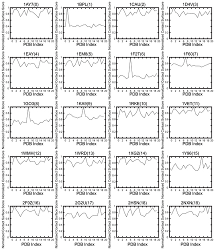
The polygonal lines of 12 out of 20 receptors have no characteristic peak. For these receptors, the score of each predicted ligand is not the maximum (ie, S_PSC < 1.0) or the number of ligands with maximal score is not only one: 1AY7³²(index = 0), 1CAU³³(2), 1D4V³⁴(3), 1EAY³⁵(4), 1EM8³⁶(5), 1VET³⁷(11), 1WMH³⁸(12), 1WRD³⁹(13), 1XG2⁴⁰(14), 2F9Z⁴¹(16), 2HSN⁴²(18), and 2NXN⁴³(19). Thus, when using only the normalized S_PSC, it is too difficult to evaluate and quantify the affinity between ligand and receptor.

Using our affinity calculation, Figures 3 and 4 show the affinity score S_affinity with w_c = 0 and w_s = 1. These values for w_c and w_s (parameters used for calculating affinity scores) were chosen to provide the maximum prediction performance (ie, F-measure) from our preliminary experiments.

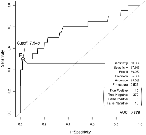
Figure 3 Affinity score S_affinity of the receptor of each ligand. The cutoff value is 7.54σ. The filled arrowhead (▾) denotes a protein pair in which S_affinity ≥ 7.54σ and is thus biologically relevant; the unfilled arrowhead is a protein pair incorrectly identified as being biologically relevant (ie, false positive). The horizontal axis shows the PDB index, and the vertical axis shows the affinity score S_affinity.

Abbreviation: PDB, Protein Data Bank.

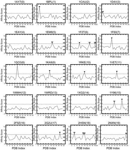
Figure 4 Matrix of affinity score S_affinity with weighting parameters w_c = 0, and w_s = 1. The points on the diagonal line show the biologically relevant pairs, and the circles show the biologically relevant pairs where the AEP system provided a successful prediction.

Abbreviation: AEP, affinity evaluation and prediction.

Figure 3 shows the S_affinity of the receptor of each ligand, and the vertical axis shows the S_affinity and the horizontal axis shows the PDB index of the receptor. When our AEP system is used as a prediction system, the horizontal dotted line shows that the cutoff value at which the system achieves its maximum prediction performance is 7.54σ. This value provides the optimal tradeoff between sensitivity and specificity. Each filled arrowhead (▾) denotes a protein pair where S_affinity exceeds the chosen cutoff value, thus indicating that the biologically relevant pair with a statistically significant score; each unfilled arrowhead is a protein pair incorrectly identified as being biologically relevant (ie, false positive).

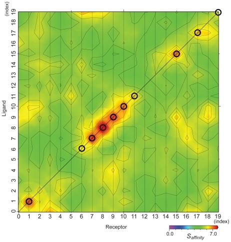
Figure 4 shows the S_affinity matrix in which the 10 data points (denoted by circles) along the diagonal of the matrix represent the protein pairs that have been experimentally confirmed to be biologically relevant. The vertical axis shows the index of the ligand, and the horizontal axis that of the receptor.

Based on Figures 2 and 3, the S_affinity obtained by our grouping process is more suitable than the simple S_PSC for estimating protein–protein affinity. For example, the S_affinity for a specific ligand is the highest for the following receptors: 1BPL⁴⁴(1), 1F60⁴⁵(7), 1GO3⁴⁶(8), 1KA9⁴⁷(9), 1RKE⁴⁸(10), 1VET(11), 1Y96⁴⁹(15), 2G2U⁵⁰(17), and 2NXN(19). These protein pairs with the highest score are also biologically relevant pairs. Moreover, for 1F2T⁵¹(6), the S_affinity of a biologically relevant pair is the 2nd high score.

Our AEP system can therefore constitute a prediction system if we introduce a recall, a precision and a cutoff value. Our system predicts pairs whose S_affinity exceeds the cutoff value and are thus biologically relevant pairs. Based on the ROC curve in Figure 5, a cutoff value of 7.54σ demonstrates the maximal prediction performance of our system. When this cutoff is adopted, the performance of our AEP as a prediction system has an F-measure of 0.526, a recall of 50.0%, a precision of 55.6% (sensitivity of 50.0% and a specificity of 97.9%), and an accuracy of 95.5%. When we consider that the prevalence of the current sample size is 5%, this performance is sufficiently high. Our AEP system identified 10 of 20 biologically relevant combinations from among 400 pairs of combination candidates. In addition, because our AEP system can identify the true negative pairs, the specificity and the accuracy are sufficiently high at 97.9%, 95.5%, respectively. This means that the prediction provided by our AEP system is reliable.

Figure 5 The ROC curve for the prediction performance of the AEP system. The peak performance achieved at point P (cutoff value is 7.54σ), and their values are shown in the bottom-right corner.

Abbreviations: AEP, affinity evaluation and prediction; ROC, receiver operating characteristics.

Efficacy of “asymmetrically biased” PSC score function for affinity analysis results by comparison of molecular size

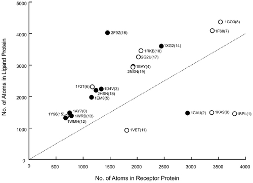
We compiled the relationship between the number of atoms in terms of a molecular size and the results of the affinity analysis as shown in Figure 6. There is a relation between the affinity results and the size of receptors or ligands. This size indicates the number of atoms for a protein. The correlation coefficient between the identification probability of biologically relevant pairs and the size of receptor is 0.40. This positive correlation is related to the characteristic of the score function of the shape complementarity. As mentioned above, the score function we used for the receptor is different from that for the ligand. Because the score function for a receptor has a “bias” that tends to pull into the ligand to own pocket structure, we expect our AEP system to exhibit increasing docking structure accuracy when searching between a “large” receptor and a “small” ligand. The current results reveal the efficacy as regards the evaluation of affinity. Moreover, because this characteristic is always good for a molecule that consists of a large number of atoms, to make the estimation performance more accurate, the dataset should be rearranged in terms of the assignment of either a receptor or a ligand by the order of the molecular size. In other word, a “large” molecule should always be assigned as a receptor regardless of whether it functions biologically as a receptor or a ligand.

Figure 6 Relation between the size of each protein pair (ie, number of atoms) needed for biological relevance and the affinity analysis results. The horizontal axis shows the number of atoms in the receptor, and the vertical axis shows that in the ligand. The symbols denote the protein pair. The unfilled circles (○) denote a protein pair that was identified as biologically relevant by the AEP system, and the filled circles (●) denotes a protein pair identified as not biologically relevant.

Abbreviation: AEP, affinity evaluation and prediction.

Problem with shape complementarity evaluation

In the current affinity analysis, our AEP system succeeded in predicting the following 10 biologically relevant protein pairs from 400 (ie, 20 × 20) protein pairs: 1BPL(1), 1F2T(6), 1F60(7), 1GO3(8), 1KA9(9), 1RKE(10), 1VET(11), 1Y69(15), 2G2U(17), and 2NXN(19). The common feature of those complex structures is that, except for 1F2T(6) and 1Y96(15), they have a typical docking type that we called “surface-to-surface”. The ”surface-to-surface” type as shown in Figure 7(a) is docking formed under a wide contact surface. Even the affinity evaluation was derived from a shape complementarity search, because in practice, the affinity analysis revealed that a shape complementarity search can identify a pair with such a docking type in a sophisticated manner from 400 protein pair candidates.

Figure 7 Models for docking styles. Type (a), called “surface-to-surface”, is most popular docking among our docking complex structures. Type (b) is called “edged-to-edge” contacting only using each edge of receptor and ligand. Type (c) is called “point-to-point” which is most less performance by shape complementarity search.

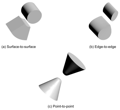
In addition, the docking type of 1F2T(6) or 1Y96(15) is different from the typical type as mentioned above. We call their docking type “edge-to-edge”. The “edge-to-edge” type is a docking style where the edge of the surface of a receptor comes in contact with a ligand edge as shown in Figure 7(b). Naturally, a shape complementarity search has difficulty in dealing with the “edge-to-edge” docking type. Indeed as shown in Figure 3, with 1F2T(6), even our AEP system succeeded in predicting the pair, and the affinity score from the correct pair is the 2nd highest score rather than the highest. Our AEP system also succeeded for 1Y96(15), however, the 2nd highest score from an irrelevant pair is also over the cutoff value of 7.54σ.

On the other hand, our AEP system failed to predict the following 10 biologically relevant pairs: 1AY7(0), 1CAU(2), 1D4V(3), 1EAY(4), 1EM8(5), 1WHM(12), 1WRD(13), 1XG2(14), 2F9Z(16), and 2HSN(18). This prediction failure might be due to a structural feature of the protein pair that hinders the shape complementarity evaluation.

Because the docking type of 1AY7(0), 1CAU(2), 1EAY(4), 1WHM(12), 1WRD(13), 1XG2(14), and 2F9Z(16) is “edge-to-edge”, the affinity scores S_affinity are low (ie, under 7.54σ) for almost all the ligands. The complex structures of 1D4V(3), 1EM8(5), and 2HSN(18) are “point-to-point” docking type. This docking type has a smaller contact surface area than the “edge-to-edge” type as shown in Figure 7(c). In fact, the docking site of the 1EM8(5) receptor is too small to allow us to detect the correct pair. This makes a shape complementarity search difficult to perform with this type.

Most of the protein pairs that our AEP system failed to predict were not the typical docking type (ie, surface-to-surface) with a complex formation as mentioned above but edge-to-edge and/or point-to-point type, because the shape complementarity search cannot deal easily with these types. We are now extracting the common characteristics from these negative docking types and developing methods to overcome these issues.

Conclusion

A shape complementarity search method and a statistical method called ‘grouping’ were combined to evaluate and predict the affinity between various protein pairs with known structures. At a prevalence of 5.0%, prediction with our AEP system had a recall of 50.0%, a precision of 55.6% and an accuracy of 95.5%. An evaluation of the affinity was difficult when only the PSC score based on the shape complementarity evaluation was considered.

The affinity evaluation was significantly improved by the grouping process that we introduced. Future research will be undertaken on the relation between the physicochemical characteristic of proteins and the prediction accuracy of our AEP system, and then, based on those findings, research will be undertaken on further improving the accuracy of the system. Although an unbound dataset was not considered in this study, our future research will also include how to improve the prediction accuracy of an unbound dataset.

Disclosure

The authors report no conflicts of interest in this work.