On calculating the probability of a set of orthologous sequences

Abstract

Probabilistic DNA sequence models have been intensively applied to genome research. Within the evolutionary biology framework, this article investigates the feasibility for rigorously estimating the probability of a set of orthologous DNA sequences which evolve from a common progenitor. We propose Monte Carlo integration algorithms to sample the unknown ancestral and/or root sequences a posteriori conditional on a reference sequence and apply pairwise Needleman–Wunsch alignment between the sampled and nonreference species sequences to estimate the probability. We test our algorithms on both simulated and real sequences and compare calculated probabilities from Monte Carlo integration to those induced by single multiple alignment.

Keywords:

• evolution
• Jukes-Cantor model
• Monte Carlo integration
• Needleman-Wunsch alignment
• orthologous

Introduction

Comparative genomics/proteomics research often focuses on a set of orthologous sequences arising from evolutionary speciation. For example, multiple related species (for example, human, mouse, and rat) can have a common gene as well as the corresponding promoters in the upstream region of such a gene, although these matched sequences may have minor difference across species. For simplicity the set of sequences studied in the sequel are assumed to have almost equal length in light of these examples. Sequence alignment algorithms¹ have substantially facilitated comparative genomics/proteomics research by showing conservation pattern along orthologous sequences, and biologically functional segments are likely to be those more conserved regions along the genome. For the vast body of related literature, we refer to Liu and colleagues,² Kellis and colleagues,³ Moses and colleagues,⁴ Xie and colleagues,⁵ Wei and Jensen,⁶ Sinha and He,⁷ and many others. As another major tool, statistical modeling approaches are devoted to comprehensively describing the probabilistic uncertainties linked to those established biological evolution models which may include two topological structures: parallel and phylogenic models (see Figure 1).

Figure 1 Evolution models.

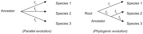
The joint parallel evolution process probability Pr(Ancestor, Species 1, 2, and 3) is

$\text{Pr}(\text{Ancestor})\prod _{i=1}^3\text{Pr}\hspace{0.17em}(\text{Species\hspace{0.17em}}i\mid \text{Ancestor}),$(1)

and the joint phylogenic evolution process probability Pr(Root, Ancestor, Species 1, 2, 3) is

$\text{Pr}(\text{Root})\text{Pr}(\text{Species\hspace{0.17em}}1\mid \text{Root})\text{Pr}(\text{Ancestor}\mid \text{Root})\prod _{i=2}^3\text{Pr}\hspace{0.17em}(\text{Species\hspace{0.17em}}i\mid \text{Ancestor}).$(2)

Jukes and Cantor⁸ proposed the first probabilistic nucleotide evolution model which assumes substitution to take place randomly among four types of nucleotides “A[1]T[2]C[3]G[4]”. The transition (from nucleotide i to nucleotide j) probability up to time t is derived as

$\begin{array}{l}{p}_{ij}(t)=(1/4)+(3/4)e^{-4\alpha t}\hspace{0.17em}\text{for\hspace{0.17em}}(i=j),\text{and}\\ (1/4)-(1/4)e^{-4\alpha t}\hspace{0.17em}\text{for\hspace{0.17em}}(i\ne j).\end{array}$(3)

We assume that the substitution rate parameter (α) is constant for different species and the evolution duration (t) is represented by specific time period (t₀, t₁, t₂, or t₃) for the associated divergence process (see Figure 1). Our question is how to effectively estimate the marginal probability for the given orthologous species sequence set without knowing the genotype of the ancestor and/or root.

Material and methods

For the unknown ancestor sequence, we simply assume that the nucleotide on any site follows a tetranomial distribution with categories {ATCG} and equal proportion, (1/4). We further assume that each nucleotide on the ancestor sequence evolves independently (under the probability law, Eq. (3)$\begin{array}{l}{p}_{ij}(t)=(1/4)+(3/4)e^{-4\alpha t}\hspace{0.17em}\text{for\hspace{0.17em}}(i=j),\text{and}\\ (1/4)-(1/4)e^{-4\alpha t}\hspace{0.17em}\text{for\hspace{0.17em}}(i\ne j).\end{array}$(3) ), so that each species sequence is a series of nucleotides which follow another tetranomial distribution identically and independently. The state space is {ATCG} and the state proportions are (P_A, P_T, P_C, P_G) which can be calculated by

$p_j=\sum _{i=1}^4(1/4)p_{ij}(t)=1/4,i,j\in \{1234\}=\{ATCG\}.$(4)

Thus, each species’ nucleotide follows the same tetranomial distribution as the ancestor nucleotide. Under the independence assumption, the probability for the species sequence is simply a product of all nucleotide marginal probabilities, (1/4). This formulation can also be used to sample the unknown ancestor state among {ATCG} given the reference species state j = (A, T, C or G), since the posterior distribution among {ATCG} for the unknown ancestor state can be easily derived to be

$p(i\mid j)=p_{ij}(t)/\sum _{k=1}^4{p}_{kj}\hspace{0.17em}(t),i=1,2,3,4.$(5)

We now briefly investigate the ambiguity extent to which different sources of sequence are aligned. For simplicity, we use the Jukes and Cantor⁸ model and assume the ancestor vs species nucleotide identity (“ancestor = species”) probability is

$1-3p,$(6)

which equals p_ii (t), in Eq. (3)$\begin{array}{l}{p}_{ij}(t)=(1/4)+(3/4)e^{-4\alpha t}\hspace{0.17em}\text{for\hspace{0.17em}}(i=j),\text{and}\\ (1/4)-(1/4)e^{-4\alpha t}\hspace{0.17em}\text{for\hspace{0.17em}}(i\ne j).\end{array}$(3) , the substitution probability is p, which equals p_ij (t) in Eq. (3)$\begin{array}{l}{p}_{ij}(t)=(1/4)+(3/4)e^{-4\alpha t}\hspace{0.17em}\text{for\hspace{0.17em}}(i=j),\text{and}\\ (1/4)-(1/4)e^{-4\alpha t}\hspace{0.17em}\text{for\hspace{0.17em}}(i\ne j).\end{array}$(3) for i ≠ j. The identity probability between two species (“species = species”) nucleotides with equal evolution duration is thus

${(1-3p)}^2+3p^2.$(7)

The statistical sequence evolution model works on probabilistic transition from the ancestor nucleotide to species nucleotide. Since the ancestor sequence is never known for a direct alignment, we may sample it a posteriori given the reference species nucleotide. The probability for event “X”, nucleotide identity between such a posterior ancestor nucleotide and another species’ nucleotide (“posterior ancestor = species”) other than the reference species nucleotide, is derived as

$\begin{array}{l}\text{Pr}(\text{reference\hspace{0.17em}species}=\text{another\hspace{0.17em}species})\\ \times \text{Pr}(\text{X}\mid \text{reference\hspace{0.17em}species}=\text{another\hspace{0.17em}species})\\ +\text{Pr}(\text{reference\hspace{0.17em}species}\ne \text{another\hspace{0.17em}species})\\ \times \text{Pr}(\text{X}\mid \text{reference}\hspace{0.17em}\text{species}\ne \text{another\hspace{0.17em}species})\\ =\left({(1-3p)}^2+3p^2\right)(1-3p)+\left(1-{(1-3p)}^2-3p^2\right)p\\ =-48p^3+36p^2-9p+1.\end{array}$(8)

The three identity probabilities (Eqs. (6)$1-3p,$(6) , (7)${(1-3p)}^2+3p^2.$(7) , and (8)$\begin{array}{l}\text{Pr}(\text{reference\hspace{0.17em}species}=\text{another\hspace{0.17em}species})\\ \times \text{Pr}(\text{X}\mid \text{reference\hspace{0.17em}species}=\text{another\hspace{0.17em}species})\\ +\text{Pr}(\text{reference\hspace{0.17em}species}\ne \text{another\hspace{0.17em}species})\\ \times \text{Pr}(\text{X}\mid \text{reference}\hspace{0.17em}\text{species}\ne \text{another\hspace{0.17em}species})\\ =\left({(1-3p)}^2+3p^2\right)(1-3p)+\left(1-{(1-3p)}^2-3p^2\right)p\\ =-48p^3+36p^2-9p+1.\end{array}$(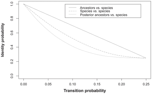8) ) are plotted in Figure 2 where the ancestor-to-species transition probability (p) varies. We find that, the identity probabilities for these three types of matched nucleotides follow the order

Figure 2 Identity probabilities for matched nucleotide pair (“ancestor vs species,” “species vs species” and “posterior ancestor vs species”).

$\begin{array}{l}\text{Pr}(\text{ancestor}=\text{species})>\text{Pr}(\text{species}=\text{species})\\ >\text{Pr}(\text{posterior\hspace{0.17em}ancestor}=\text{species}),\end{array}$

or

$(6)>(7)>(8).$

Thus, alignment between the ancestor and species sequences may be less ambiguous than between two species sequences. Figure 2 also indicates that, the difference among these three types of identity probability is most significant in the middle of interval (0, 1/4). The dominance of “Pr(ancestor = species) over Pr (reference species = another species)” is more significant than that of “Pr (reference species = another species) over Pr (posterior ancestor = another species)”, and the difference between the lower two curves (Figure 2) seems not to be relatively large. Thus pairwise alignment between the posterior ancestor and another species sequence may achieve similar unambiguity as alignment between species.

Now we study a multispecies orthologous sequence set (say Human = Species 1, Mouse = Species 2, and Rat = Species 3 in Figure 1). We denote by B_a, B₁, B₂, and B₃ the sequences of the unknown ancestor, Species 1, 2, and 3. Under the nucleotide substitution model and unambiguous matching, the probability for the set of sequences under parallel evolution is

$\begin{array}{l}P(B_1,B_2,B_3)={\sum }_{B_a}P(B_1,B_2,B_3\mid B_a)\pi (B_a)\\ ={\sum }_{B_a}P(B_1\mid B_a)P(B_2\mid B_a)\\ \times P(B_3\mid B_a)\pi (B_a),\end{array}$(9)

where π (·) is the identical and independent tetranomial distribution for the ancestor nucleotide with state space {ATCG} and equal (1/4) proportion. The result is obtained by integrating out four possible ancestor nucleotides on each site for a marginal nucleotide group (three members across species) probability and multiplying these individual marginal probabilities along the sequence. Similarly, the phylogenic evolution model requires integrating out both the ancestor and root nucleotides on each site to get the result. Note that multiple alignment is not needed under the substitution model since no gaps are allowed. For general nucleotide substitution–insertion–deletion, the probabilistic evolution model developed by Rivas⁹ gives the overall “substitution, insertion, and deletion” probabilities from the ancestor to species given divergence time. Calculating the evolution probability from the ancestor (assumed to be known) to the observed species sequence using the Rivas⁹ model may require multiple alignments up front in order to match those nucleotides between the ancestor and species. Aside from not knowing the ancestor sequence, unambiguous alignment may not exist due to moderate sequence divergence.⁷ Thus, one can underestimate the sequence set probability which is induced in a similar way to Eq. (9)$\begin{array}{l}P(B_1,B_2,B_3)={\sum }_{B_a}P(B_1,B_2,B_3\mid B_a)\pi (B_a)\\ ={\sum }_{B_a}P(B_1\mid B_a)P(B_2\mid B_a)\\ \times P(B_3\mid B_a)\pi (B_a),\end{array}$(9) because it simply picks one alignment to calculate the sequence set probability without incorporating other possible alignments. Ignoring ambiguous alignment may also lead to incorrect phylogenic inference and/or misleading sequence taxa partition pattern.^10,11 Under a moderate sequence length (~100 nucleotides), a tetranomial distribution for each nucleotide along the ancestor sequence may be used to sample ancestor nucleotides independently to form a large number (n) of sequences which are further used to induce a probabilistically evolved set of species sequences based on the Rivas⁹ model. The sequence set probability is simply estimated as the number of exact duplicates of the given sequence set divided by n. However, this is highly impractical under moderate sequence length due to the small chance of duplicate sequence sets. Another possible way is applying pairwise alignment between each sampled ancestor sequence and observed species-specific sequences, and the sequence set probability may be done by averaging these evolution probabilities over all sampled ancestor sequences.

However, this may also be inefficient due to non-informative ancestor sampling and lack of reliable alignment between a random sequence and species sequences. Thus it becomes desirable to propose and investigate more efficient multiple-imputation-like approaches such as using posterior ancestor samples which may offer multiple representative alignment results conditional on a reference species sequences for sequence set probability elicitation. Instead of following the theme of Eq. (9)$\begin{array}{l}P(B_1,B_2,B_3)={\sum }_{B_a}P(B_1,B_2,B_3\mid B_a)\pi (B_a)\\ ={\sum }_{B_a}P(B_1\mid B_a)P(B_2\mid B_a)\\ \times P(B_3\mid B_a)\pi (B_a),\end{array}$(9) , we turn to calculating P (B₁, B₂, B₃) in an alternative way under parallel evolution

$\begin{array}{l}P(B_1,B_2,B_3)=P(B_2,B_3\mid B_1)P(B_1)\\ =\left[{\sum }_{B_a}P(B_2,B_3\mid B_a)P(B_a\mid B_1)\right]\\ \times \left[{\sum }_{B_a}P(B_1\mid B_a)\pi (B_a)\right]\\ =\left[{\sum }_{B_a}P(B_2\mid B_a)P(B_3\mid B_a)P(B_a\mid B_1)\right]\\ \left[{\sum }_{B_a}P(B_1\mid B_a)\pi (B_a)\right]\\ =[I]\times [II],\end{array}$(10)

where [II] is obtained after multiplicity over all nucleotide marginal probabilities for Species 1 (see Eq. (4)$p_j=\sum _{i=1}^4(1/4)p_{ij}(t)=1/4,i,j\in \{1234\}=\{ATCG\}.$(4) ). As for [I], since B_a (posterior ancestor) is sampled from the reference sequence (offspring) B₁ and the integrand is the offspring (B₂, B₃) probability derived from the representative ancestor B_a which is already linked to offspring B₁ through posterior sampling. Monte Carlo integration introduced in Eq. (10)$\begin{array}{l}P(B_1,B_2,B_3)=P(B_2,B_3\mid B_1)P(B_1)\\ =\left[{\sum }_{B_a}P(B_2,B_3\mid B_a)P(B_a\mid B_1)\right]\\ \times \left[{\sum }_{B_a}P(B_1\mid B_a)\pi (B_a)\right]\\ =\left[{\sum }_{B_a}P(B_2\mid B_a)P(B_3\mid B_a)P(B_a\mid B_1)\right]\\ \left[{\sum }_{B_a}P(B_1\mid B_a)\pi (B_a)\right]\\ =[I]\times [II],\end{array}$(10) realistically implements the joint probability of multiple post-evolution sequences by working on pairwise alignments between the sampled ancestor sequence and observed species-specific sequences. Under phylogenetic (tree-structured) evolution (the right panel in Figure 1), the sequence set probability can be written as

$\begin{array}{l}P(B_1,B_2,B_3)=P(B_2,B_3\mid B_1)P(B_1)\\ =\left[{\sum }_{B_r,B_a}P(B_2,B_3\mid B_r,B_a)P(B_r,B_a\mid B_1)\right]\\ \times \left[{\sum }_{B_r}P(B_1\mid B_r)\pi (B_r)\right]\\ =\left[{\sum }_{B_r,B_a}P(B_2,B_3\mid B_r,B_a)P(B_a\mid B_r)P(B_r\mid B_1)\right]\\ \times \left[{\sum }_{B_r}P(B_1\mid B_r)\pi (B_r)\right]\\ =\left[{\sum }_{B_r,B_a}P(B_2,B_3\mid B_a)P(B_a\mid B_r)P(B_r\mid B_1)\right]\\ \times \left[{\sum }_{B_r}P(B_1\mid B_r)\pi (B_r)\right]\\ =\left[{\sum }_{B_r,B_a}P(B_2\mid B_a)P(B_3\mid B_a)P(B_a\mid B_r)P(B_r\mid B_1)\right]\\ \times \left[{\sum }_{B_r}P(B_1\mid B_r)\pi (B_r)\right]\\ =[I]\times [II],\end{array}$(11)

where B₁ is Species 1 (Human) sequence, B_r is the root sequence, and B_a is the ancestor sequence in Figure 1. However, if we use Species 2 (Mouse) sequence B₂ as the reference sequence, then we have the following decomposition

$\begin{array}{l}P(B_1,B_2,B_3)=P(B_1,B_3\mid B_2)P(B_2)\\ =\left[{\sum }_{B_r,B_a}P(B_1,B_3\mid B_r,B_a)P(B_r,B_a\mid B_2)\right]\\ \times \left[{\sum }_{B_r}P(B_2\mid B_r)\pi (B_r)\right]\\ =\left[{\sum }_{B_r,B_a}P(B_1\mid B_r)P(B_3\mid B_a)P(B_r,B_a\mid B_2)\right]\\ \times \left[{\sum }_{B_r}P(B_2\mid B_r)\pi (B_r)\right]\end{array}$(12)

Note that,

$P(B_r,B_a\mid B_2)=P(B_r\mid B_a)(B_a\mid B_2)$

and

$\sum _{B_r}P(B_2\mid B_r)\pi (B_r)=\sum _{B_r}\left[\sum _{B_a}P(B_2\mid B_a)P(B_a\mid B_r)\right]\pi (B_r).$(13)

As in Eq. (4)$p_j=\sum _{i=1}^4(1/4)p_{ij}(t)=1/4,i,j\in \{1234\}=\{ATCG\}.$(4) , we assign 1/4 to the probability for each nucleotide along the reference sequence B₂ after applying Eq. (13)$\sum _{B_r}P(B_2\mid B_r)\pi (B_r)=\sum _{B_r}\left[\sum _{B_a}P(B_2\mid B_a)P(B_a\mid B_r)\right]\pi (B_r).$(13) . Only pairwise alignment between the posterior ancestor sequence and species sequence is used for Monte Carlo integration (Eqs. (10)$\begin{array}{l}P(B_1,B_2,B_3)=P(B_2,B_3\mid B_1)P(B_1)\\ =\left[{\sum }_{B_a}P(B_2,B_3\mid B_a)P(B_a\mid B_1)\right]\\ \times \left[{\sum }_{B_a}P(B_1\mid B_a)\pi (B_a)\right]\\ =\left[{\sum }_{B_a}P(B_2\mid B_a)P(B_3\mid B_a)P(B_a\mid B_1)\right]\\ \left[{\sum }_{B_a}P(B_1\mid B_a)\pi (B_a)\right]\\ =[I]\times [II],\end{array}$(10) , (11)$\begin{array}{l}P(B_1,B_2,B_3)=P(B_2,B_3\mid B_1)P(B_1)\\ =\left[{\sum }_{B_r,B_a}P(B_2,B_3\mid B_r,B_a)P(B_r,B_a\mid B_1)\right]\\ \times \left[{\sum }_{B_r}P(B_1\mid B_r)\pi (B_r)\right]\\ =\left[{\sum }_{B_r,B_a}P(B_2,B_3\mid B_r,B_a)P(B_a\mid B_r)P(B_r\mid B_1)\right]\\ \times \left[{\sum }_{B_r}P(B_1\mid B_r)\pi (B_r)\right]\\ =\left[{\sum }_{B_r,B_a}P(B_2,B_3\mid B_a)P(B_a\mid B_r)P(B_r\mid B_1)\right]\\ \times \left[{\sum }_{B_r}P(B_1\mid B_r)\pi (B_r)\right]\\ =\left[{\sum }_{B_r,B_a}P(B_2\mid B_a)P(B_3\mid B_a)P(B_a\mid B_r)P(B_r\mid B_1)\right]\\ \times \left[{\sum }_{B_r}P(B_1\mid B_r)\pi (B_r)\right]\\ =[I]\times [II],\end{array}$(11) , and (12)$\begin{array}{l}P(B_1,B_2,B_3)=P(B_1,B_3\mid B_2)P(B_2)\\ =\left[{\sum }_{B_r,B_a}P(B_1,B_3\mid B_r,B_a)P(B_r,B_a\mid B_2)\right]\\ \times \left[{\sum }_{B_r}P(B_2\mid B_r)\pi (B_r)\right]\\ =\left[{\sum }_{B_r,B_a}P(B_1\mid B_r)P(B_3\mid B_a)P(B_r,B_a\mid B_2)\right]\\ \times \left[{\sum }_{B_r}P(B_2\mid B_r)\pi (B_r)\right]\end{array}$(12) ). Since the probability of a sequence evolving from an ancestor is obtained by multiplying over all individual nucleotide evolution probabilities along a sequence, a large sequence length (say >100) may result in an overly small probability and lead to numerical overflow. The log-probability (LogPr) for a species evolutionary sequence from the ancestor is the summation of individual nucleotide evolutionary log-probabilities, and the evolutionary probability expectation obtained from Monte Carlo integration (exp(LogPr) mean), can be implemented by using moment generating function with argument one. Normality of these randomly produced LogPrs leads to the simple result of exp (μ + σ²/2) where μ and σ² are the sample mean and variance for these LogPrs.

Simulation and real data study

We first introduce in detail the extended Jukes and Cantor model by Rivas⁹ which will be used for our simulation study. The transition probabilities among general states {–ATCG} (“–” is the gap or covalent bond between two nucleotides) until time t are

$\left[\begin{array}{llllll}\hfill & -\hfill & A\hfill & T\hfill & C\hfill & G\hfill \\ -\hfill & \sigma (t)\hfill & \xi (t)\hfill & \xi (t)\hfill & \xi (t)\hfill & \xi (t)\hfill \\ A\hfill & \gamma (t)\hfill & r(t)\hfill & s(t)\hfill & s(t)\hfill & s(t)\hfill \\ T\hfill & \gamma (t)\hfill & s(t)\hfill & r(t)\hfill & s(t)\hfill & r(t)\hfill \\ C\hfill & \gamma (t)\hfill & s(t)\hfill & s(t)\hfill & r(t)\hfill & s(t)\hfill \\ G\hfill & \gamma (t)\hfill & s(t)\hfill & s(t)\hfill & s(t)\hfill & r(t)\hfill \end{array}\right],$(14)

where the {–ATCG} column to the left of the transition probability matrix represents the initial (ancestor) states and the {–ATCG} row on top of the matrix represents the final (species) states. Specifically,

$\{\begin{array}{l}r(t)=(1/4)e^{-\beta t}+(3/4)e^{-(4\alpha +\beta )t};\hfill \\ S(t)=(1/4)e^{-\beta t}-(1/4)e^{-(4\alpha +\beta )t};\hfill \\ \gamma (t)=1-e^{-\beta t};\hfill \\ \xi (t)=(1/4)(1-q_0)e^{-\beta t};\hfill \\ \sigma (t)=1-(1-q_0)e^{-\beta t}.\hfill \end{array}$(15)

For these generalized transition probabilities, we refer to the notations from the substitution model (Eq. (3)$\begin{array}{l}{p}_{ij}(t)=(1/4)+(3/4)e^{-4\alpha t}\hspace{0.17em}\text{for\hspace{0.17em}}(i=j),\text{and}\\ (1/4)-(1/4)e^{-4\alpha t}\hspace{0.17em}\text{for\hspace{0.17em}}(i\ne j).\end{array}$(3) ) and denote the element (u, v) in the matrix (Eq. (14)$\left[\begin{array}{llllll}\hfill & -\hfill & A\hfill & T\hfill & C\hfill & G\hfill \\ -\hfill & \sigma (t)\hfill & \xi (t)\hfill & \xi (t)\hfill & \xi (t)\hfill & \xi (t)\hfill \\ A\hfill & \gamma (t)\hfill & r(t)\hfill & s(t)\hfill & s(t)\hfill & s(t)\hfill \\ T\hfill & \gamma (t)\hfill & s(t)\hfill & r(t)\hfill & s(t)\hfill & r(t)\hfill \\ C\hfill & \gamma (t)\hfill & s(t)\hfill & s(t)\hfill & r(t)\hfill & s(t)\hfill \\ G\hfill & \gamma (t)\hfill & s(t)\hfill & s(t)\hfill & s(t)\hfill & r(t)\hfill \end{array}\right],$(14) ) to be p _{−1, v−1}(t), where u (row index) and v (column index) = 1, 2, 3, 4, 5. Parameter 0 < q₀ ≤ 1 controls the background (nongap) frequency at time t. Specifically, letting β = 0 leads to the original Jukes and Cantor model (Eq. (3)$\begin{array}{l}{p}_{ij}(t)=(1/4)+(3/4)e^{-4\alpha t}\hspace{0.17em}\text{for\hspace{0.17em}}(i=j),\text{and}\\ (1/4)-(1/4)e^{-4\alpha t}\hspace{0.17em}\text{for\hspace{0.17em}}(i\ne j).\end{array}$(3) ) and q₀ = 1 excludes nucleotide insertion. Since each pair of neighboring ancestor nucleotides holds a potential insertion site (gap, “–”) with an overall “gap:nongap” ratio of one, we assume a pentanomial distribution for general ancestor nucleotide states with sample space {–[0]A[1]T[2]C[3]G[4]} and normalized probability set (p₀ = 1/2, p₁ = p₂ = p₃ = p₄ = 1/8). This assumption is useful for sampling the posterior ancestor state among {–ATCG} given the reference species state (–, A, T, C or G). If we denote the general species nucleotide state to be J ε {–ATCG}, then the posterior distribution among {–ATCG} for the unknown ancestor state is

$P(i\mid j)=p_i{p}_{ij}(t)/\sum _{k=0}^4{p}_k\hspace{0.17em}{p}_{kj}(t),i=0,1,2,3,4.$(16)

Parallel evolution model

We refer to the left panel of Figure 1.

1. Simulate the ancestor sequence with length = L₀;

2. Simulate species “1, 2, 3” sequences from this simulated ancestor sequence;

3. Apply Monte Carlo integration to randomly produced log(evolution probabilities) for Species 2 and 3 conditional on Species 1 sequence, where the unknown ancestor sequences are sampled using Eq. (16)$P(i\mid j)=p_i{p}_{ij}(t)/\sum _{k=0}^4{p}_k\hspace{0.17em}{p}_{kj}(t),i=0,1,2,3,4.$(16) with corresponding divergence time;

4. As a numerical verification, we apply Monte Carlo integration to randomly produced log(evolution probabilities) for Species 1 and 3 conditional on Species 2 sequence, where the unknown ancestor sequences are sampled using Eq. (16)$P(i\mid j)=p_i{p}_{ij}(t)/\sum _{k=0}^4{p}_k\hspace{0.17em}{p}_{kj}(t),i=0,1,2,3,4.$(16) with corresponding divergence time;

5. As another numerical verification, we apply Monte Carlo integration to randomly produced log(evolution probabilities) for Species 1 and 2 conditional on Species 3 sequence, where the unknown ancestor sequences are sampled using Eq. (16)$P(i\mid j)=p_i{p}_{ij}(t)/\sum _{k=0}^4{p}_k\hspace{0.17em}{p}_{kj}(t),i=0,1,2,3,4.$(16) with corresponding divergence time;

6. We investigate the consistency among different references.

7. Various divergence time vector (t₁, t₂, t₃) in the left panel of Figure 1 and transition parameter (β and q₀ in Eq. (15)$\{\begin{array}{l}r(t)=(1/4)e^{-\beta t}+(3/4)e^{-(4\alpha +\beta )t};\hfill \\ S(t)=(1/4)e^{-\beta t}-(1/4)e^{-(4\alpha +\beta )t};\hfill \\ \gamma (t)=1-e^{-\beta t};\hfill \\ \xi (t)=(1/4)(1-q_0)e^{-\beta t};\hfill \\ \sigma (t)=1-(1-q_0)e^{-\beta t}.\hfill \end{array}$(15) ) configurations are given in Table 1, where transition parameter (α in Eq. (15)$\{\begin{array}{l}r(t)=(1/4)e^{-\beta t}+(3/4)e^{-(4\alpha +\beta )t};\hfill \\ S(t)=(1/4)e^{-\beta t}-(1/4)e^{-(4\alpha +\beta )t};\hfill \\ \gamma (t)=1-e^{-\beta t};\hfill \\ \xi (t)=(1/4)(1-q_0)e^{-\beta t};\hfill \\ \sigma (t)=1-(1-q_0)e^{-\beta t}.\hfill \end{array}$(15) ) is standardized into one unit.

   Table 1 Simulation configurations (parallel [PA] and phylogenic [PH] evolution models, α = 1.0)

   No	β	t0	t1	t2	t3	q0	L0
   		(PA, PH)	(PA, PH)	(PA, PH)	(PA, PH)
   1	0.05	N/A, 0.05	0.10, 0.10	0.10, 0.05	0.10, 0.05	0.95	100
   2	0.05	N/A, 0.05	0.10, 0.10	0.20, 0.15	0.10, 0.05	0.95	100
   3	0.05	N/A, 0.10	0.20, 0.20	0.20, 0.10	0.20, 0.10	0.95	100
   4	0.20	N/A, 0.15	0.30, 0.30	0.30, 0.15	0.30, 0.15	0.90	100
   5	0.20	N/A, 0.15	0.30, 0.30	0.60, 0.45	0.30, 0.15	0.90	100
   6	0.20	N/A, 0.01	0.05, 0.05	0.05, 0.04	0.05, 0.04	0.80	100
   7	0.05	N/A, 0.05	0.10, 0.10	0.10, 0.05	0.10, 0.05	0.95	500
   8	0.05	N/A, 0.05	0.10, 0.10	0.20, 0.15	0.10, 0.05	0.95	500
   9	0.05	N/A, 0.10	0.20, 0.20	0.20, 0.10	0.20, 0.10	0.95	500
   10	0.20	N/A, 0.15	0.30, 0.30	0.30, 0.15	0.30, 0.15	0.90	500
   11	0.20	N/A, 0.15	0.30, 0.30	0.60, 0.45	0.30, 0.15	0.90	500
   12	0.20	N/A, 0.01	0.05, 0.05	0.05, 0.04	0.05, 0.04	0.80	500

Phylogenic evolution model

We refer to the right panel of Figure 1.

1. Simulate root sequence with length = L₀ and the evolved ancestor sequence for Species 2 and 3;

2. Simulate Species 1 sequence from this simulated root sequence, and simulate the Species 2 and 3 sequences from this simulated ancestor sequence;

3. Apply Monte Carlo integration to randomly produced log(evolution probabilities) for Species 2 and 3 conditional on Species 1 sequence, where the unknown root and ancestor sequences are sampled using Eq. (16)$P(i\mid j)=p_i{p}_{ij}(t)/\sum _{k=0}^4{p}_k\hspace{0.17em}{p}_{kj}(t),i=0,1,2,3,4.$(16) with corresponding divergence times;

4. As a numerical verification, we apply Monte Carlo integration to randomly produced log(evolution probabilities) for Species 1 and 3 conditional on Species 2 sequence, where the unknown root and ancestor sequences are sampled using Eq. (16)$P(i\mid j)=p_i{p}_{ij}(t)/\sum _{k=0}^4{p}_k\hspace{0.17em}{p}_{kj}(t),i=0,1,2,3,4.$(16) with corresponding divergence times;

5. As another numerical verification, we apply Monte Carlo integration to randomly produced log(evolution probabilities) for Species 1 and 2 conditional on Species 3 sequence, where the unknown root and ancestor sequences are sampled using Eq. (16)$P(i\mid j)=p_i{p}_{ij}(t)/\sum _{k=0}^4{p}_k\hspace{0.17em}{p}_{kj}(t),i=0,1,2,3,4.$(16) with corresponding divergence times;

6. We investigate the consistency among different references.

7. Various divergence time vector (t₀, t₁, t₂, t₃) in the right panel of Figure 1 and transition parameter (β and q₀ in Eq. (15)$\{\begin{array}{l}r(t)=(1/4)e^{-\beta t}+(3/4)e^{-(4\alpha +\beta )t};\hfill \\ S(t)=(1/4)e^{-\beta t}-(1/4)e^{-(4\alpha +\beta )t};\hfill \\ \gamma (t)=1-e^{-\beta t};\hfill \\ \xi (t)=(1/4)(1-q_0)e^{-\beta t};\hfill \\ \sigma (t)=1-(1-q_0)e^{-\beta t}.\hfill \end{array}$(15) ) configurations are given in Table 1, where transition parameter (α in Eq. (15)$\{\begin{array}{l}r(t)=(1/4)e^{-\beta t}+(3/4)e^{-(4\alpha +\beta )t};\hfill \\ S(t)=(1/4)e^{-\beta t}-(1/4)e^{-(4\alpha +\beta )t};\hfill \\ \gamma (t)=1-e^{-\beta t};\hfill \\ \xi (t)=(1/4)(1-q_0)e^{-\beta t};\hfill \\ \sigma (t)=1-(1-q_0)e^{-\beta t}.\hfill \end{array}$(15) ) is standardized into one unit. We use the same transition parameter (β and q₀ in Eq. (15)$\{\begin{array}{l}r(t)=(1/4)e^{-\beta t}+(3/4)e^{-(4\alpha +\beta )t};\hfill \\ S(t)=(1/4)e^{-\beta t}-(1/4)e^{-(4\alpha +\beta )t};\hfill \\ \gamma (t)=1-e^{-\beta t};\hfill \\ \xi (t)=(1/4)(1-q_0)e^{-\beta t};\hfill \\ \sigma (t)=1-(1-q_0)e^{-\beta t}.\hfill \end{array}$(15) ) from the parallel model simulation and make evolution divergence times comparable between the parallel and phylogenic models.

We collect LogPrs from 1000 Monte Carlo simulations. The distribution of these LogPrs are plotted in Figures 3, 4, 5 and 6. A Kolmogorov–Smirnov normality test gives p-value (>0.15) for all LogPr sets, which means that the difference between the produced LogPrs and a normally distributed random variable is not significant. The normality assumption for LogPrs holds and the probability approximation based on log-normal distribution is reasonable. For such an assumption, a heuristic justification without rigorous theoretical proof is as follows: Given each randomly produced ancestor sequence, each nucleotide (event) LogPr on the non-reference sequences acts as an independently and identically distributed random variable, and the summation of these LogPrs follows the central limit theorem for a large sample size (sequence length). By increasing the ancestor or root length from 100 to 500, we can see that the relationship between LogPr and the sequence length is approximately linear. Another observation from Tables 2 and 3 is that different reference species sequences may lead to inconsistent sequence set probabilities due to different evolution durations and/or topological locations within the phylogenic structure. The phylogenic evolution model (the right panel of Figure 1) seems to show more inconsistency than the parallel evolution model (the left panel of Figure 1) does due to the dual missing sequences (the root and ancestor) instead of ancestor only in the parallel evolution model. A reference sequence which is closer to the root and/or ancestor is preferable since the imputed multiple roots and/or ancestors tend to be more informative due to shorter divergence. The CLUSTAL W multiple alignment¹²- induced probability is obtained by moving along the sequence set which holds nucleotides {ATCG} and possible gaps (covalent bonds) and applying Rivas⁹ model, where “one gap with two nucleotides” across three matched sequence sites stands for a deletion and “two gaps with one nucleotide” across three matched sequence sites stands for an insertion. For each simulated sequence set, the discrepancy between Monte Carlo integration (MCI) and single multiple alignment (MA) induced probabilities are clearly more significant than that among probabilities estimated from different reference species sequences.

Figure 3 Log(probability) densities from parallel model 1–6.

Notes: Solid line, Species 1; dashed line, Species 2; dotted line, Species 3.

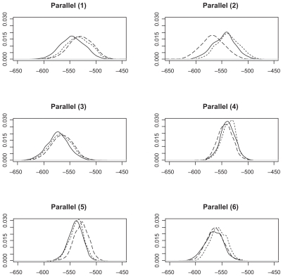
Figure 4 Log(probability) densities from parallel model 7–12.

Notes: Solid line, Species 1; dashed line, Species 2; dotted line, Species 3.

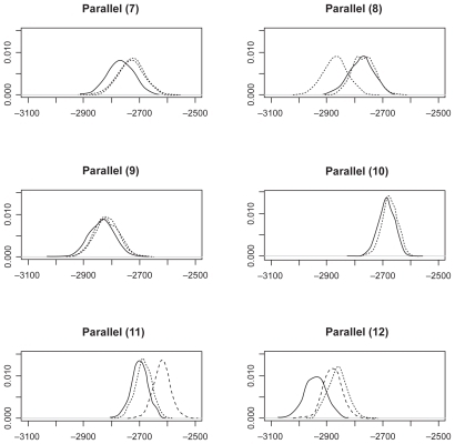
Figure 5 Log(probability) densities from phylogenic model 1–6.

Notes: Solid line, Species 1; dashed line, Species 2; dotted line, Species 3.

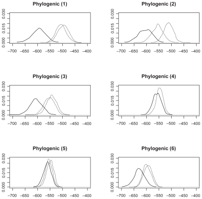
Figure 6 Log(probability) densities from phylogenic model 7–12.

Notes: Solid line, Species 1; dashed line, Species 2; dotted line, Species 3.

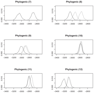
Table 2 Computation results (parallel evolution models)

No	Mean (Log(probability))	0.5 variance (Log(probability))	Log(probability) (MCI)	Length (MA)	Log(probability) (MA)
	Reference species: 1, 2, and 3
1	−544, −528, −533	267, 257, 263	−277, −270, −270	104	−1343
2	−545, −567, −538	229, 252, 231	−317, −315, −307	104	−1343
3	−572, −565, −568	197, 205, 212	−376, −361, −356	109	−1344
4	−538, −543, −536	92, 99, 87	−447, −444, −450	112	−1143
5	−539, −528, −537	88, 100, 91	−450, −429, −446	108	−1118
6	−565, −563, −556	152, 130, 119	−413, −432, −437	123	−1056
7	−2767, −2727, −2734	1135, 1130, 1121	−1632, −1597, −1613	536	−6825
8	−2775, −2868, −2766	1026, 970, 853	−1748, −1898, −1913	535	−6823
9	−2835, −2815, −2822	1008, 937, 853	−1827, −1879, −1969	533	−6801
10	−2684, −2683, −2673	434, 459, 412	−2249, −2225, −2261	533	−5786
11	−2700, −2620, −2685	455, 451, 429	−2245, −2170, −2257	538	−5678
12	−2940, −2878, −2860	763, 535, 580	−2177, −2342, −2280	630	−5413

Abbreviations: MCI, Monte Carlo integration; MA, multiple alignment.

Table 3 Computation results (phylogenic evolution model)

No	Mean(Log(probability))	0.5 variance (Log(probability))	Log(probability) (MCI)
	Reference species: 1, 2, and 3
1	−596, −506, −496	402, 219, 218	−193, −287, −279
2	−604, −554, −511	378, 253, 180	−227, −301, −331
3	−607, −553, −543	302, 215, 195	−305, −338, −348
4	−557, −545, −546	140, 93, 99	−417, −452, −447
5	−562, −550, −556	119, 100, 95	−443, −450, −461
6	−628, −597, −593	229, 134, 136	−399, −464, −456
7	−3063, −2696, −2697	1425, 1029, 1016	−1638, −1667, −1680
8	−3049, −2923, −2763	1041, 1074, 888	−2008, −1849, −1875
9	−3002, −2904, −2884	1072, 992, 937	−1930, −1912, −1948
10	−2782, −2768, −2766	545, 420, 410	−2237, −2348, −2356
11	−2804, −2745, −2801	491, 437, 439	−2314, −2308, −2362
12	−3215, −3087, −3077	928, 585, 598	−2287, −2502, −2479

Abbreviation: MCI, Monte Carlo integration.

CREB promoters study

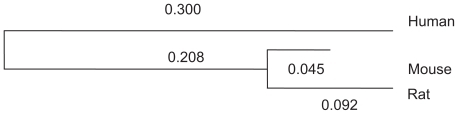
From the ABS database,¹³ we extracted the promoter regions of transcription factor CREB for three mammals (human, mouse and rat). We used MEGA 4.1 package¹⁴ to construct the phylogeny tree with corresponding divergence times under uniform transition rate 1 (see Figure 7). These are used for sampling the posterior ancestor and root.

Figure 7 Phylogeny tree for orthologous CREB promoters.

Since no current packages give us β and q₀ maximum likelihood estimation for Rivas⁹ model (Eq. (14)$\left[\begin{array}{llllll}\hfill & -\hfill & A\hfill & T\hfill & C\hfill & G\hfill \\ -\hfill & \sigma (t)\hfill & \xi (t)\hfill & \xi (t)\hfill & \xi (t)\hfill & \xi (t)\hfill \\ A\hfill & \gamma (t)\hfill & r(t)\hfill & s(t)\hfill & s(t)\hfill & s(t)\hfill \\ T\hfill & \gamma (t)\hfill & s(t)\hfill & r(t)\hfill & s(t)\hfill & r(t)\hfill \\ C\hfill & \gamma (t)\hfill & s(t)\hfill & s(t)\hfill & r(t)\hfill & s(t)\hfill \\ G\hfill & \gamma (t)\hfill & s(t)\hfill & s(t)\hfill & s(t)\hfill & r(t)\hfill \end{array}\right],$(14) ), we mainly investigate the sequence set probability sensitivity to β and q₀ input by trying different values. We report the means and variances as well as estimated Log(sequence set probabilities) under two parameter settings for β and q₀ under different reference species. We also report the p-values from Kolmogorov–Smirnov normality test (Table 4). The normality test results are sensitive to parameter input and reference species selection, which may be due to the fact that conservation levels/transition probabilities are likely to be nonhomogeneous along the sequences. Two LogPr distributions under associated parameter inputs are plotted in Figure 8. As a verification, we apply multiple alignment to these three promoters and at each site we calculate the nucleotide identity proportion within the window (with size 23) starting from this site at the gene direction (Figure 9). The conservation levels show that evolutionary transition rates are approximately constant piece-wisely, thus the central limit theorem discussed for the simulated data study may still apply to these LogPrs on each promoter segment with quasi-constant conservation level under certain nucleotide insertion-deletion parameter (β, q₀) values.

Figure 8 Distribution of LogPrs (CREB promoters).

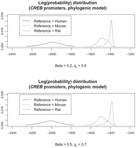
Figure 9 Nucleotide identity proportion along the upstream promoter regions for transcription factor CREB.

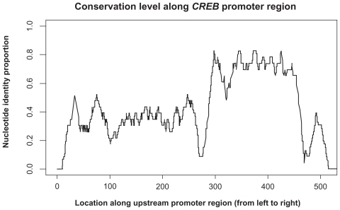
Table 4 Computation results for CREB promoter sequence set (phylogenic evolution models)

β, q0	Mean (Log(probability))	0.5 variance (Log(probability))	Log(probability) (MCI)	p-value
Reference species: 1, 2, and 3
0.2, 0.7	−1912, −1408, −1462	5724, 249, 656	3812, −1159, −806	= 0.11, <0.01, <0.01
0.3, 0.7	−1964, −1403, −1467	5015, 259, 777	3051, −1144, −690	>0.15, <0.01, <0.01
0.4, 0.7	−1998, −1401, −1467	4506, 307, 958	2508, −1094, −518	= 0.04, <0.01, <0.01
0.5, 0.7	−2017, −1400, −1487	4501, 345, 1049	2484, −1055, −438	<0.01, <0.01, >0.15
0.2, 0.8	−1789, −1361, −1424	5231, 742, 927	3442, −619, −497	>0.15, <0.01, <0.01
0.3, 0.8	−1833, −1358, −1432	4892, 781, 1056	3059, −577, −376	>0.15, <0.01, = 0.04
0.4, 0.8	−1816, −1359, −1446	4240, 822, 1207	2424, −537, −239	>0.15, <0.01, >0.15
0.5, 0.8	−1880, −1361, −1460	4334, 827, 1251	2454, −534, −209	>0.15, <0.01, >0.15

Abbreviation: MCI, Monte Carlo integration.

Discussion

We proposed and investigated some promising numerical algorithms for accurately estimating the probability of a set of orthologous sequences with equal length under certain assumptions. Our approach was to informatively shuffle the unknown ancestors and/or roots and to find the distributional characteristics of simulated log-probabilities in order to reasonably approximate the true probability. The merit of our approach depends on how well the ancestor and/or root is imputed based on certain pentanomial distribution proportions (p₋, p_A, p_T, p_C, p_G) in Eq. (16)$P(i\mid j)=p_i{p}_{ij}(t)/\sum _{k=0}^4{p}_k\hspace{0.17em}{p}_{kj}(t),i=0,1,2,3,4.$(16) using the evolution model⁹ and how reliably the pairwise Needleman-Wunsch alignment is applied to cross-species matching of nucleotides which are supposed to come from the same ancestor entry {–, A, T, C or G}. The former depends on the divergence duration from the ancestor/root to the reference sequence and the latter may depend on the species-specific adjustment of pairwise alignments based on phylogenic information. When this piece of information is not immediately available, the algorithms by Yang,¹⁵ Redelings and Suchard,¹¹ and MEGA package¹⁴ are useful. Recently, Wong and colleagues¹⁶ demonstrated that various alignments may lead to quite inconsistent inference. Although distance estimation for multiple species from a common ancestor may lack some accuracy using only one sequence set (Figure 9), we used MEGA package for phylogenic structure information for real sequence set probability estimation. Note that we only use background sequences as examples to demonstrate our algorithms by assuming independent tetranomial distribution among {ATCG} along sequences. For the set of orthologous sequences involving many species (>3), we follow the evolutionary process (described by a phylogenic tree) to sample the internal nodes within the phylogenic tree conditional on one selected reference sequence (a terminal node on the phylogenic tree) and apply Monte Carlo integration to these imputed internal nodes for obtaining LogPrs (we omit the details). As one referee points out, it may be unreliable to directly apply our algorithms to sequences with very irregular lengths, since the insertion–deletion events need to be identified by matching nucleotides across all involved species other than due to artificial sequence truncation. Thus a crude multiple alignment across such sequences may overly produce insertion and/or deletions. A rough solution may involve first applying multiple alignment procedures to these sequences and then segmenting the aligned sequences into subsequences involving different numbers of species followed by segment-wise Monte Carlo integration. However, the internal edge-effects introduced by segmentation deserves further study. Lastly, we highlight that applying the proposed algorithms to real sequences is not so straightforward in view of heterogeneous conservation patterns along the orthologous sequences, which poses as an important future research topic.

Acknowledgments

We thank Terence P Speed for his directions on evolution models when he visited Yale Center for Statistical Genomics and Proteomics (YCSGP) in May 2004. We are also grateful to Stéphane Robin and many anonymous referees for their constructive and insightful comments which greatly improved our work.

Disclosure

The authors report no conflicts of interest in this work.