The route to diabetes: Loss of complexity in the glycemic profile from health through the metabolic syndrome to type 2 diabetes

Abstract

Aims:

In many physiologic systems, the evolution from health to disease correlates with a loss of complexity in the system’s output. We analyze the difference in complexity of the glycemic profile in healthy volunteers (H), patients with the metabolic syndrome (MS), and patients with type 2 diabetes mellitus (DM).

Methods:

We measured interstitial fluid glucose every 5 minutes for 3 days in 10 H, 10 MS, and 10 DM. Complexity of the glycemic profile was evaluated by means of detrended fluctuation analysis (DFA). Mean amplitude of glycemic excursions (MAGE) was also calculated.

Results:

Glucose profile was more complex (lower DFA) in healthy subjects than in patients with MS or DM (mean DFA [SD]: H: 1.25 (0.10), MS: 1.39 (0.07), DM: 1.42 (0.10). ANOVA: F_2,27 = 9.94, p = 0.001). DM had also a less complex profile than MS, but this difference was not statistically significant. There was an inverse relation between complexity (lower DFA) and the number of MS defining criteria (rho = 0.55, p = 0.002) and between complexity and MAGE (r = 0.68, p < 0.0001).

Conclusions:

There is a progressive loss of complexity in the glycemic profile from health, through the metabolic syndrome to type 2 diabetes mellitus. This loss of complexity precedes hyperglycemia and correlates with other markers of disease progression. Complexity analysis may be a useful tool to track the evolution from health to type 2 diabetes. Furthermore, it may provide a way to measure glycemic control in real-life situations and has some distinct advantages over other conventional variability metrics.

Keywords:

• complexity
• metabolic syndrome
• type 2 diabetes mellitus
• detrended fluctuation analysis
• glycemic profile

Introduction

Type 2 diabetes mellitus (DM) affects about 5% of adults worldwide, and this prevalence is rising rapidly (Secree and Zimmet 2003). Individuals with impaired fasting glucose (IFG) or impaired glucose tolerance are asymptomatic but are at high risk of future type 2 diabetes and vascular disease (Unwin et al 2002). Nevertheless, these definitions of prediabetes have limitations and even the current cut-off levels proposed by the American Diabetes Association for IFG (fasting plasma glucose >100 mg/dl) are open to debate (Cheng et al 2006; Andreozzi et al 2007; Nichols et al 2007; Rijkelijkhuizen et al 2007).

During the past few years, the term “metabolic syndrome” (MS) has been increasingly used in medical literature. It describes the clustering in an individual of several traits, including insulin resistance, obesity, hypertension, and dyslipidemia, which are all highly prevalent in the Western lifestyle and each represent a major risk factor for cardiovascular disease (WHO 1999; NCEP 2002). Several recent reports show that the metabolic syndrome is associated with a large increase in the risk of cardiovascular events (Lakka et al 2002; Girman et al 2004) and several pieces of evidences suggest a common pathophysiological background for this syndrome, at the center of which lies insulin resistance (Zimmet 1992). Patients with the MS are also at increased risk of developing DM (Hanley et al 2004).

The MS is very prevalent in developed countries (Ford and Giles 2003; Park et al 2003). The increasing burden of obesity worldwide is the driving force behind the rising prevalence of the DM and MS (Park et al 2003; Carr et al 2004).

The progress from normal health through the MS to overt DM is arguably a gradual evolution, and its division into distinct steps is probably artificial. A smoother, more quantitative approach may provide a better description of this evolution. Unfortunately, the hallmark of this progress, insulin resistance, is not easy to measure in real-life conditions. We intend to ascertain whether complexity analysis may provide a new tool to describe this process.

Complex biological systems are characterized by a highly elaborate output. Often, one of the first symptoms of disease is a “decomplexification” of this output, due to uncoupling or loss of its processing capacities (Goldberger 1997; Goldberger et al 2002). Complexity analysis techniques may provide an easy and sensitive way of displaying this phenomenon (Varela et al 2005, 2006).

This is probably the case in the evolution from health through MS until DM. Namely, we suggest that the derangement of glucose metabolism that underlies this evolution is displayed as a gradual and progressive loss of complexity in the glycemic time series as each patient walks his way from normality to full-blown DM.

We intend to develop an instrument that may give some quantitative insight into the evolution from the normal, healthy state through the MS to DM, in real-life conditions. We correlate this tool with a classic measure of variability: the mean amplitude of glycemic excursions (MAGE). This metric has been used to assess acute glucose fluctuations and was found to be related with activation of oxidative stress markers in DM (Monnier et al 2006).

Patients and methods

Ten successive patients with the MS (defined by National Cholesterol Education Program – Adult Treatment Panel III (NCEP-ATPIII) criteria (Secree and Zimmet 2003), excluding type 2 diabetes) and 10 successive patients with DM (defined as fasting plasma glucose ≥126 mg/dl in two consecutive occasions and/or on antidiabetic treatment) were selected from the outpatient internal medicine and vascular risk clinics of a urban 400-bed teaching hospital in Madrid, Spain. Only patients with a recent diagnosis of DM (less than one year), and only on dietary or oral antidiabetic treatment were selected. 10 healthy volunteers were used as controls. To avert the influence of gender and hormonal status, only men were selected. We intentionally chose early DM to highlight the possible differences in these first stages of DM. The study was approved by the Hospital’s Ethics Committee, and an informed consent was obtained from each patient.

The characteristics of patients and controls are displayed in Table 1.

Table 1 Patient’s characteristics

	Healthy controls (H)	Metabolic syndrome (MS)	Type 2 diabetes (DM)
Age (yr)	45.2 (17.3)	50.7 (11.9)	59.7 (7.2)	F2,27^Table Footnote* = 4.08, p = 0.028	H-DM p = 0.022
BMI (Kg/m2)	26.2 (3.0)	33.3 (4.9)	29.8 (5.8)	F2,27^Table Footnote* = 5.49, p = 0.010	H-MS p = 0.007
Waist (cm)	94 (16.4)	112.4 (13.6)	107.2 (11.6)	F2,27^Table Footnote* = 5.34, p = 0.011	nsd
Systolic BP (mm Hg)	142 (28.1)	148 (20.6)	144 (25.1)	nsd
Diastolic BP (mm Hg)	83 (9.3)	90 (13.4)	83 (11.7)	nsd
Glucose (mmol/L)	5.46 (0.40)	5.97 (0.69)	7.47 (1.31)	F2,27^Table Footnote* = 14.37, p < 0.001	H-DM p = 0.001; MS-DM p = 0.002
HDL-C (mmol/l)	1.33 (0.21)	1.19 (0.21)	1.39 (0.39)	nsd
Triglycerides (mmol/L)	1.11 (0.37)	1.50 (0.61)	1.49 (0.68)	nsd
Glycosylated Hb (%)	5.3 (0.5)	5.9 (0.3)	6.8 (1.1)	F2,27^Table Footnote* = 10.68, p < 0.001	H-DM p = 0.001; MS-DM p = 0.030
Insulin (pmol/L)	51 (16)	107 (83)	101 (77)	KW nsd
HOMA-IR	2.1 (0.7)	4.6 (3.2)	5.6 (4.5)	KW† Chi2 = 8.43, p = 0.015
DFA	1.39 (0.10)	1.39 (0.07)	1.42 (0.10)	F2,27^Table Footnote* = 9.94, p = 0.001	H-DM p = 0.001; MS-DM p = 0.006
MAGE	30.0 (14.3)	45.5 (17.2)	62.7 (27.5)	F2,27^Table Footnote* = 6.38, p = 0.005	H-DM p = 0.004

Abbreviations: BMI, body mass index; BP, blood pressure; DFA, detrended fluctuation analysis; HDL-C, high-density lipoprotein-cholesterol; HOMA-IR, Homeostatic Assessment Model of Insulin Resistance; MAGE, mean amplitude of glycemic excursions.

Notes:

* ANOVA,

† Kruskal-Wallis.

Units conversion: Glucose (mg/dl) = Glucose (mmol/L) * 18.02; HDL-C (mg/dl) = HDL-C (mmol/L) * 38.61; Triglycerides (mg/dl) = Triglycerides (mmol/L) * 88.50; Insulin (uU/ml) = Insulin (pmol/L) * 0.1667.

On admission to the study, after a full clinic exam, blood was extracted to measure basic biochemical parameters (including fasting plasma glucose, glycosylated hemoglobin, insulin, and lipids). Then a sensor was inserted in the abdominal subcutaneous tissue, and interstitial glucose was recorded every 5 minutes for at least 48 hours (CGMS System Gold, Medtronic MiniMed, Medtronic Diabetes, Northridge, CA, USA). Subjects were asked to record at least 3 fingerstick measurements daily. Otherwise, patients carried on with their normal ambulatory life, followed their normal treatment, and were not required to take any special care.

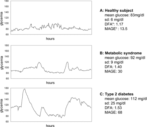
A glucose time series was obtained from each subject. From this series, we extracted a 24-hour long series (from 06.00 AM on day 2 to 06.00 AM on day 3) for study. We selected day 2 to avert the stressing influences of insertion and laboratory exams, and we excluded day 4 because of the concern of claudication of the capillary probe. Figure 1 shows an example of a healthy subject, a patient with the MS, and a patient with DM.

Figure 1 Example of a glycemic profile of a patient of each group.

Notes: *DFA, detrended fluctuation analysis; ^†MAGE, mean amplitude of glycemic excursions.

Conventional statistics (mean or median, standard deviation [SD], or interquartile range) were recorded from the time series. MAGE was calculated according to Service and colleagues (1987).

Complexity analysis

The complexity of the glucose profile was evaluated by means of detrended fluctuation analysis (DFA). DFA is a well established technique to measure the complexity of a time series. An in-depth discussion on DFA is outside the scope of this paper, and may be seen in Peng and colleagues (2000). A summary is presented in the Appendix. Very schematically, DFA analyses how a time series and its linear regression diverge as the “time window” increases. Intuitively, DFA can be conceived as representing the span of influence of the different points in a time series. In a series with high complexity, the influence of each point rapidly fades away, while in a “smoother” series the influence of each point lasts longer. As a rule of thumb, higher complexities are displayed as lower DFA (until a minimum of 0.5).

Statistics

Differences among groups were evaluated by means of ANOVA, with post-hoc analysis (Tukey) when necessary. Univariate ANOVA was used to correct for other covariables. When normality conditions were not fulfilled, Kruskal-Wallis test was employed.

Spearman correlation was used to analyze the relation between complexity and the number of metabolic syndrome-defining criteria.

Linear regression was used to correlate DFA and MAGE.

In every case, statistical significance was assumed if p < 0.05. The statistical software employed was SPSS version 12 (SPSS Inc., Chicago, IL, USA).

Results

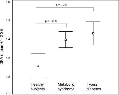
The patient’s characteristics are displayed in Table 1. The glucose profile was clearly more complex (ie, lower DFA) in healthy subjects than in patients with the metabolic syndrome or in diabetic patients (mean DFA [SD] in healthy controls: 1.25 (0.10), MS: 1.39 (0.07), DM 1.42 (0.10); ANOVA: F_2,27 = 9.94, p = 0.001). In the post-hoc analysis, healthy subjects differed both from patients with the MS (p = 0.006) and with DM (p = 0.001). Diabetic patients had also a less complex profile than patients with the metabolic syndrome, but this difference did not achieve statistical significance (Figure 2). This results did not change significantly when corrected for the effect of age (ANOVA F_2,26 = 8.72, p = 0.002), body mass index (F_2,26 = 8.06, p = 0.002), waist circumference (F_2,26 = 7.85, p = 0.002), or fasting plasma glucose (F_2,26 = 4.90, p = 0.016). Also, correcting for systolic or diastolic blood pressure, total cholesterol, high-density lipoprotein-cholesterol, low-density lipoprotein-cholesterol, or triglycerides did not change significantly these results (F > 7.80, p < 0.002 in every case). If the whole time series recorded was analyzed (in stead of just the second day), the results were similar (DFA in healthy controls:1.26 [SD 0.05]; MS:1.36 [SD 0.05]; DM:1.42 [SD 0.07]).

Figure 2 Differences in detrended fluctuation analysis among healthy subjects, patients with the metabolic syndrome and patients with type 2 diabetes.

There was a statistically significant inverse relation between profile complexity and the number of metabolic syndrome defining criteria (NCEP-ATPIII criteria [Secree and Zimmet 2003] (rho = 0.55, p = 0.002). These results did not differ if patients with full blown DM were excluded (rho = 0.58, p = 0.008), nor when adjusted for age (rho = 0.55, p = 0.002).

By way of contrast, variability, as measured through MAGE, increased from health (30.0 [SD 14.3]) to MS (45.5 [17.2]) and DM (62.7 [27.5]). With ANOVA, the post-hoc analysis could differentiate between healthy subjects and diabetic patients, but it could not discriminate between healthy subjects and MS or between MS and DM. These results did not change significantly when correcting for age, body mass index, or waist circumference, but when correcting for fasting glucose, MAGE became nonsignificant (F_2,26 = 0.551, p = 0.58).

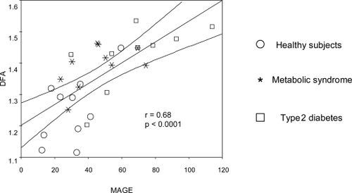
A highly significant correlation was observed between DFA and MAGE (r = 0.68, p < 0.0001): high variability correlated with high DFA (and thus, low complexity) (Figure 3)

Figure 3 Correlation between detrended fluctuation analysis and mean amplitude of glycemic excursions.

Discussion

The evolution from health to DM seems to be marked by a progressive loss of complexity in the glycemic profile, probably reflecting increasing insulin resistance and a failing glucoregulation. This loss of complexity appears well before the development of hyperglycemia. Overall, our MS patients had a fasting plasma glucose lower than 110 mg/dl, and 40% of them less than 100 mg/dl.

We did not find significant differences in the glycemic profile complexity in MS patients when compared with DM. However, the significant inverse correlation between the complexity of the glycemic profile and the number of MS criteria in each patient suggests that the path from health through the MS to DM is more a quantitative than a qualitative change, and highlights the fuzziness of their limits.

Blood glucose variability has recently emerged as an important variable in critical care both in diabetic and nondiabetic patients (Egi et al 2006), as well as an independent risk factor for diabetic complications in DM (Saudek et al 2006). We found a tight inverse correlation between glycemic variability (measured with MAGE) and complexity (measured with DFA). It would seem as if all through the evolution from health to full-blown DM, the glucoregulatory system became progressively more “sloppy” and slow-reacting, and required bigger departs from baseline to launch a counteregulatory response. Thus, although the coincidence of increased variability and loss of complexity may at first glance seem contradictory, it probably represents just two different aspects of the same disorder, namely, the loss of fine regulation on glycemic levels.

Complexity measures may have some advantages over classic MAGE. In the first place, it is less operator-dependent. In order to measure MAGE, each peak has to be assessed as to decide whether it qualifies as an excursion. Furthermore, the qualifying limit (usually, 1 SD) is arbitrary, and minor imprecisions on this measure have substantial consequences on the results. Finally, the discriminant power of MAGE depends heavily on plasma glucose, and correcting for this variable invalidates its diagnostic capacity.

By way of contrast, DFA is not operator-dependent and does not depend on an arbitrary limit. Furthermore, it explores the glucoregulatory response throughout the whole time series, thereby analyzing all the span of glycemic variations and not just the biggest ones.

It could be argued that the loss of complexity observed in MS and DM may be an artifact due to differences in body composition. Both groups have higher body mass index and probably their subcutaneous tissue will have an increase adiposity that could influence the sampling of interstitial fluid. Nevertheless, adjusting for body mass index or waist circumference does not significantly change the results.

Recently, Ogata and colleagues (2006, 2007) analyzed diabetes-related alterations of glucose control by means of DFA on a continuous glucose monitoring system. Their results on healthy volunteers (DFA 1.25 [SD 0.29]) are almost identical to ours. DFA in diabetic patients is slightly higher in their series (DFA 1.65 [0.30] vs 1.42 [0.10]), probably reflecting more advanced diabetes. These authors propose that the break down of the physiologic negative long-range correlation in glycemia observed in patients with diabetes proves that the net effects of the flux and reflux persist for many hours and may reflect a central pathogenic mechanism in diabetes, ie, the lack of tight control in blood glucose. These observations support our hypothesis that new metrics derived from complexity analysis could improve diagnostic and prognostic work-up in diabetes, and help in the understanding of glucose dysregulation in this disease.

An objection that can be raised is that subjects did not follow a standardized life regime, and variation on meals or activity may confound our results. Nevertheless, we tried to develop a real-life model, displaying what happens in normal life, easy to apply in daily practice, rather than a research instrument.

Also, it could be argued that glucose levels in interstitial fluid may not accurately reflect plasma levels, and that our results may show differences in the plasma/interstitium kinetics rather than in plasmatic values. Obviously, this caveat would also apply to other routine uses of CGMS (ie, insulin dose adjustment, insulin infusion pumps, etc) that don’t consider these limitations.

In conclusion, if corroborated, complexity analysis of the glycemic profile may provide a useful technique to track the evolution from health through the MS to DM in real-life conditions. Glucose instability and its contribution to diabetic cardiovascular risk could also be assessed in this way. Furthermore, complexity analysis may be helpful in the evaluation of the new “insulin-sensitizing” drugs and their possible contribution in improving glucoregulation.

Acknowledgments

We acknowledge Maria Jose Lopez Ribera and Guadalupe Castro Toril for their help in the data collection. The authors declare no conflicts of interest in this work.

Appendix

Detrended fluctuation analysis

Detrended fluctuation analysis (DFA) attempts to disclose patterns of self-similarity in time plots. That is, it looks for the presence of “memory” in the curve; memory understood as long-range correlations.

In order to be able to perform DFA, it is first necessary to integrate the time series:$y(k)={\sum }_{i=1}^k({\text{G}}_{\text{i}}-{\text{G}}_{\text{mean}})$(Figure 4) where G_i is each individual point and G_mean is the mean of the series as a whole.

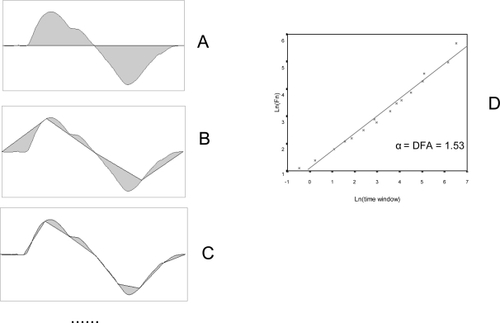
Next, the integrated curve is divided into time segments of size n (Figure 5A, B, C). A regression line is calculated for each segment, and the difference between the integrated curve and the different regression lines is computed:$\text{F}(\text{n})=\sqrt{\frac{1}{N}\sum _{k=1}^N{\left[y(k)-y_n(k)\right]}^2}$where F(n) is the measure of the difference between the integrated curve and the regression lines, N is the total curve at each point, and y_n(k) is the value of the regression number of data points, y(k) is the value of the integrated line at that point.

Figure 4 Detrended fluctuation analysis (1). From the original time series, an integrated curve is obtained:$y(k)={\sum }_{i=1}^k(G_i-G_{\mathit{\text{mean}}})$

Notes: G_i, each individual point; G_mean, mean of the series as a whole. This integrated curve will be utilized for further calculations.

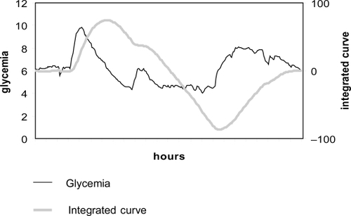
This operation is repeated for different time frames (that is, for different values of n). The smaller the time scale (n), the better the fit of the regression lines to the integrated curve, and the lower the value of F(n). Conversely, the value of F(n) tends to increase exponentially as the time frame (n) increases.

Finally, the relation between F(n) and the size of n is analyzed. A plot is drawn with log[F(n)] on the y-axis and log(n) on the x-axis (Figure 5D). A good fit to a regression line indicates the existence of scaling (self-similarity), and a fractal structure can be assumed.

DFA is the slope of the regression line (α). It displays the scaling exponent, and is an indicator of the degree of complexity of the curve. In an entirely random time series (“white noise”) α = 0.5. A 1/f type time series will have α = 1. A “random walk” (the integration of a random series, “Brown noise”) will display α = 1.5. Long range negatively correlated fluctuations will show α < 1.5, while in positive correlations α >1.5.

On the whole, a curve is more complex (less predictable) the closer its value of α is to 0.5. (Values of α lower than 0.5 reveal anticorrelations, which also implies a certain degree of predictability, and hence a lower level of complexity).

Figure 5 Detrended fluctuation analysis (DFA) (2). The integrated curve is divided into progressively smaller time segments (A, B, C, etc). A regression line is calculated for each segment, and the total difference between the integrated curve and the regression lines is calculated for each time window (F(n), gray area). The smaller the time window, the better the fit of the regression line and the lower the value of F(n). Finally, a plot is drawn (D) with log(F(n)) in the y-axis and log(time-window) in the x-axis. A good fit reveals the presence of scaling (self-similarity). DFA is the slope of the regression line. It displays the scaling exponent, and is an indicator of the degree of complexity of the curve.

In our series, N = 288.

The program used to calculate DFA was written in Python (http://www.python.org) and is available from the authors on request ([email protected]).