Two resource distribution strategies for dynamic mitigation of influenza pandemics

Abstract

As recently pointed out by the Institute of Medicine, the existing pandemic containment and mitigation models lack the dynamic decision support capabilities. We present two simulation-based optimization models for developing dynamic predictive resource distribution strategies for cross-regional pandemic outbreaks. In both models, the underlying simulation mimics the disease and population dynamics of the affected regions. The quantity-based optimization model generates a progressive allocation of limited quantities of mitigation resources, including vaccines, antiviral, administration capacities, and social distancing enforcement resources. The budget-based optimization model strives instead allocating a total resource budget. Both models seek to minimize the impact of ongoing outbreaks and the expected impact of potential outbreaks. The models incorporate measures of morbidity, mortality, and social distancing, translated into the societal and economic costs of lost productivity and medical expenses. The models were calibrated using historic pandemic data and implemented on a sample outbreak in Florida, with over four million inhabitants. The quantity-based model was found to be inferior to the budget-based model, which was advantageous in its ability to balance the varying relative cost and effectiveness of individual resources. The models are intended to assist public health policy makers in developing effective distribution policies for mitigation of influenza pandemics.

Keywords:

• pandemic
• mitigation
• distribution
• dynamic
• resources
• budget

Introduction and motivation

Influenza pandemics have historically ensued enormous societal calamities amplified by staggering economic forfeitures. In the U.S. alone, the Spanish flu (1918, serotype H1N1), the Asian flu (1957, H2N2), and the Hong Kong flu (1968, H3N2) resulted in the death toll of more than 500,000, 70,000 and 34,000 cases, respectively.¹ More recently, a series of scattered outbreaks of the avian-to-human transmittable H5N1 virus has been mapping its way through Asia, the Pacific region, Africa, the Near East, and Europe.² As of March 2010, the World Health Organization (WHO) has reported 287 deaths in 486 cases, worldwide.³ At the same time, in Spring 2009, a milder human-to-human transmissible H1N1 virus subtype resurfaced and propagated to an ongoing global outbreak; as of March 2010, 213 countries have been affected with a total number of infections and mortalities of 419,289 and 16,455, respectively.⁴ Today, most experts have an ominous expectation that the next pandemic will be triggered by an emerging highly pathogenic virus, to which there is little or no pre-existing immunity in humans.⁵

The ability to contain and mitigate influenza pandemics depends on available emergency response infrastructure and resources, and at present, challenges abound. Prediction of the exact emerging virus subtype remains a difficult task, and once it is identified, a surge production of sufficient vaccine quantities can take from six to nine months.^6,7 Even if the emerged subtype has a known epidemiology, the existing stockpiles would be limited due to high production and inventory costs.^8,9 Also will be significantly constrained the supply of antiviral, immunizers and other healthcare providers, hospital beds and supplies, and logistics. Thereby, pandemic mitigation has to be done amidst a limited knowledge of disease and population dynamics, constrained infrastructure, shortage of effective clinical treatments, and to-be-proven resource allocation policies. This challenge, faced during the recent H1N1 outbreak, has been acknowledged by WHO⁹ and echoed by the Health and Human Services (HHS) and the Center for Disease Control and Prevention (CDC).^10,11

The existing literature on pandemic influenza (PI) modeling aims to address various complex aspects of the pandemic evolution process including: (i) underlying spatio-temporal structure, (ii) contact dynamics and disease transmission, (iii) disease progression, and (iv) development of mitigation strategies. A comprehensive decision-aid model for containment and mitigation has to invariably consider all of the above aspects: it must incorporate the mechanism of disease progression, from initial infection, to the asymptomatic phase, manifestation of symptoms, and a final health outcome;^12–14 it must also consider the population dynamics, including individual susceptibility^15,16 and transmissibility,^12,17–19 as well as the behavioral factors that affect infection generation and disease progression;^20–23 finally, it must incorporate the impact of pharmaceutical and non-pharmaceutical measures, including vaccination, antiviral therapy, social distancing and travel restrictions, and use of low-cost measures, such as face masks and hand washing.^24–27

In recent years, the models for PI containment and mitigation have focused on integrating therapeutical and non-therapeutical measures in search for synergistic strategies, aimed at better resource utilization. Most of these approaches implement a form of social distancing to reduce infection exposure, followed by application of pharmaceutical means. A number of significant contributions has been made in this challenging area.^1,25,28–32 One of the most notable among the recent efforts is a 2006–07 initiative by the Models of Infectious Disease Agent Study (MIDAS)³³ which examined independent models of large-scale PI spread for rural areas of Asia,^34,35 U.S. and U.K.,^36,37 and the city of Chicago.³⁸ MIDAS cross-validated the models by simulating the city of Chicago, with 8.6 M inhabitants, and implementing targeted layered containment.^39,40 The research findings of MIDAS and other institutions^14,25 were used in a recent “Modeling Community Containment for Pandemic Influenza” report by the Institute of Medicine (IOM), to formulate a set of recommendations for mitigating PI at a local level.⁴¹ These recommendations were used in a pandemic preparedness guidance developed jointly by CDC, HHS, and other federal agencies.⁴²

At the same time, the IOM report points out several limitations of the MIDAS models, observing that “because of the significant constraints placed on the models” being considered by policy makers, “the scope of the models should be expanded.” The IOM recommends “to adapt or develop decision-aid models that can ... provide real-time feedback during an epidemic.” The report also emphasizes that “future modeling efforts should incorporate broader outcome measures ... to include the costs and benefits of intervention strategies”.⁴¹ It can indeed be observed that practically all existing approaches focus on assessment of apriori defined strategies; virtually none of the synergistic decision models are capable of “learning”, ie, adapting to changes in the pandemic course, yet predicting them, to generate a dynamic optimal strategy. Such a strategy is advantageous in its ability to be state-dependent, ie, as being formed dynamically as the pandemic spreads, by selecting the optimal combination of available mitigation options at each decision epoch, based on the present pandemic state.

In an attempt to address the IOM recommendations, we present two novel simulation-based optimization models for developing dynamic predictive resource distribution strategies for a network of regional pandemic outbreaks. In both models, the underlying simulation mimics disease and population dynamics of the affected regions (Sections 2.1 and 2.2). The quantity-based optimization model (Section 2.3) generates a progressive allocation of limited quantities of mitigation resources, including stockpiles of vaccines and antiviral, healthcare capacities for vaccination and antiviral treatment, and social distancing enforcement resources. The budget-based optimization model (Section 2.3.1) allocates a total resource budget, as opposed to a separate allocation of individual resources, which vary in their relative cost and effectiveness. Both models seek to dynamically minimize the impact of ongoing outbreaks and the expected impact of potential outbreaks, spreading from the ongoing regions. The optimality criterion incorporates measures of morbidity, mortality, and social distancing, translated into the societal and economic costs of lost productivity and medical expenses. The models were calibrated using historic pandemic data and implemented on a sample cross-regional outbreak in Florida, U.S., with over four million inhabitants (Section 3). We present a sensitivity analysis for estimating the marginal impact of changes in the total budget and quantity availability (Section 3.4), and show that the quantity-based approach is inferior to the budget-based strategy, which takes advantage of its ability to balance the relative cost and effectiveness of individual resources.

Compared to our earlier work,⁴³ this paper presents the following main advances: (i) the original single-region simulation⁴³ has been expanded to serve as the basis for the cross-regional simulation model presented in this paper; (ii) we now propose two novel dynamic optimization models, embedded in the cross-regional simulation, to generate resource distribution strategies; as such, the decision support power of our model has substantially increased; (iii) the calibration methodology now incorporates both the basic reproduction number and the infection attack rate; inclusion of the latter adds to a more accurate assessment of the pandemic severity over the entirety of the pandemic period, and (iv) our model now incorporates certain socio-behavioral features, such as the target population compliance.

Simulation-based optimization framework

Our simulation-based optimization framework generates progressive resource allocations over a network of regional outbreaks. Resources include stockpiles and capacities for vaccine and antiviral administration, and social distancing enforcement resources, among others. The framework subsumes a cross-regional simulation model, a set of single-region simulation models, and an overarching optimization control.

The regions inside the network are classified as unaffected, ongoing outbreak or contained. The cross-regional model connects the regions by air and land travel. The single-region model emulates the (hourly) population and disease dynamics of each ongoing region, affected by mitigation measures. The pandemic spreads from ongoing to unaffected regions by (a)symptomatic travelers passing through border control. At every new regional outbreak epoch, the optimization model allocates available resources to the new outbreak region (actual allocation) and unaffected regions (virtual allocation). Daily statistics are collected for each region, including the number of infected, deceased, and quarantined cases, for different age groups. As a regional outbreak is contained, its societal and economic costs are estimated.

Cross-regional simulation model

The model initializes by creating mixing groups and population dynamics for each region (see Section 2.1). A pandemic is triggered by injecting one infectious case into a randomly chosen region. The resulting regional contact dynamics and disease propagation are presented in Section 2.2. As the symptomatic cases start seeking medical assistance, the new regional outbreak is detected, and a resource allocation is generated (see Section 2.3) and passed over to the single-region model.

The outbreak spreads to unaffected regions as infectious travelers pass with some probability through border control (the probability varies with the degree of symptom manifestation). Travelers are assumed to act independently. Each traveler is assumed to seed a regional outbreak in her destination with an equal, time-homogeneous probability ω for the entirety of her infection period. For each unaffected region, the outbreak probability at time t is calculated using the binomial probability law, as follows $P_t=1-{(1-\omega )}^{n_t},$(1) where n_t denotes the number of infectious travelers in the region at time t. Based on the outbreak probability values, the model determines which of the regions have become new outbreaks (in the testbed implementation, the values of P_t were computed daily). The model also determines if an ongoing outbreak has been contained, based on a certain threshold of the daily infection rate. The cross-regional simulation stops when all outbreaks have been contained.

Single-region simulation model

The single-region simulation model mimics population and disease dynamics within the affected region.

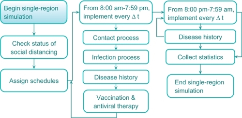
A schematic of the model is shown in Figure 1. The model subsumes the following main components: (i) population dynamics (schedules), (ii) contact and infection process, (iii) disease natural history, and (iv) mitigation prevention and intervention, including social distancing, vaccination, and antiviral application. The model collects detailed regional statistics, including numbers of infected, recovered, deceased, and quarantined cases, for different age groups. For a contained outbreak, its societal and economic costs are calculated. The societal cost includes the cost of lost lifetime productivity of the deceased; the economic cost includes the cost of medical expenses of the recovered and deceased and the cost of lost productivity of the quarantined (see Section 3.3; Meltzer 1999).⁴⁴ The single-region simulation extends our original model.⁴³

Figure 1 Schematic of single-region simulation model.

Population dynamics (schedules)

We view a region as a set of population centers formed by mixing groups (eg, households, offices, facilities, universities, dormitories, schools, shopping centers, etc.). Each individual is assigned a set of attributes (eg, age, gender, parenthood, workplace, infection susceptibility, probability of travel, etc). Each person is also assigned Δt time-discrete (eg, Δt = 1 hour) weekday and weekend schedules, which depend on: (i) person’s age and parenthood, (ii) disease status, (iii) travel status, (iv) social distancing decrees in place and person’s compliance. As their schedules advance, inhabitants circulate throughout the mixing groups. It is assumed that at any point of time, an individual belongs to one of the exclusive compartments of susceptible, infected, recovered or deceased.

Contact and infection processes

Infection transmission occurs during contact events between susceptible and infectious cases in the mixing groups. At the beginning of every Δt period (eg, one hour), for each mixing group g, the simulation tracks the total number of infectious cases, n_g, present in the group. Each infectious case generates r_g per Δt unit of time new contacts,³⁷ chosen randomly (uniformly) from the susceptible. We make the following assumptions about the contact process: (i) during Δt period, a susceptible may come into contact with at most one infectious case and (ii) each contact exposure lasts Δt units of time. Once a susceptible has started a contact exposure at time t, she will develop infection at time t + Δt with a certain probability that is calculated as shown below.

Let L_i(t) be a nonnegative continuous random variable that represents the duration of contact exposure, starting at time t, required for contact i to become infected. We assume that L_i(t) is distributed exponentially with mean 1/λ_i(t), where λ_i(t) represents the instantaneous force of infection applied to contact i at time t. ^45–47 The probability that susceptible i, whose contact exposure has started at time t, will develop infection at time t + Δt is then given as $P\{L_i(t)\le \Delta t\}=1-e^{-{\lambda }_i(t)\Delta t}.$(2)

Disease natural history

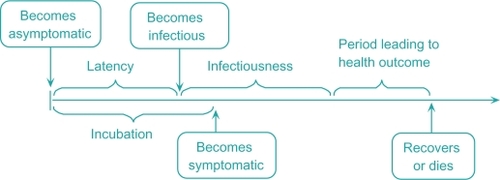
A schematic of the disease natural history is shown in Figure 2. During the incubation phase, the individual stays asymptomatic. At the end of the latency phase, she becomes infectious and enters the infectious phase.^35,37,39 She becomes symptomatic at the end of incubation. At the end of the infectious phase, she enters the final disease stage which culminates in her recovery or death.

Figure 2 Schematic of disease natural history model.

Mortality for influenza is a complex process affected by many factors and variables, most of which have limited accurate data support from past pandemics. Furthermore, the time of death can be weeks following the disease episode (often attributable to pneumonia related complications).⁴⁸ Because of the uncertainty underlying the mortality process, we thus adopted a simplified, age-based form of the mortality probability of infected i, as follows $m_i={\mu }_i-{\tau \rho }_i,$(3) where μ_i is the age-dependent base mortality probability of infected i, ρ_i is her status of antiviral therapy (0 or 1), and τ is the antiviral efficacy measured as the decrease in the base probability.³⁵ We assume that a recovered case develops immunity but continues circulating in the mixing groups.

Mitigation strategies

Mitigation include pharmaceutical and non-pharmaceutical options. It is initiated upon detection of a critical number of confirmed infected cases,⁴⁹ which triggers resource allocation and deployment. We assume a certain delay for deployment of field responders.

Pharmaceutical mitigation consists of vaccination and antiviral application. Vaccination is targeted at individuals at risk to reduce their infection susceptibility. We assume that a certain fraction of the risk group does not comply with vaccination. The vaccine takes a certain period to become effective (typically, between 10 and 14 days).⁵⁰ Vaccination is constrained by the available stockpile and administration capacity measured in terms of the number of immunizer-hours.

We assume that as some symptomatic cases seek medical assistance,^51,52 a fraction at risk of them receives an antiviral. Antiviral treatment is subject to availability of the antiviral stockpile and administration capacity, measured in terms of the number of certified providers.

Both vaccination and antiviral application are affected by social behavioral factors, including conformance of the target population, degree of risk perception, and compliance of healthcare personnel.^53–55 The conformance level of the population at risk can be affected, among other factors, by the demographics and income level^56–60 as well as the quality of public information.⁶¹ The degree of risk perception can be influenced by negative experiences developed during pharmaceutical campaigns of the previous outbreaks,^62,63 as well as by public fear and rumors.^64,65

Non-pharmaceutical mitigation includes social distancing and travel restrictions. We adopted a CDC guidance,⁴² which establishes five categories of pandemic severity and recommends quarantine and closure options according to the category. The categories are determined based on the value of the case fatality ratio (CFR), the proportion of fatalities in the total infected population. For the CFR lower than 0.1% (Category 1), voluntary at-home isolation of infected cases is implemented. If the CFR falls in-between 0.1% and 1.0% (Categories 2 and 3), in addition to the at-home isolation, the following measures are recommended: (i) voluntary quarantine of households members of infected cases and (ii) child and adult social distancing. For the CFR exceeding 1.0% (Categories 4 and 5), all the above measures are implemented. As effectiveness of social distancing is affected by some of the behavioral factors listed above,⁶¹ we assume a certain social distancing conformance level. Travel restrictions considered in the model included regional air and land border control for infected travelers.

Optimization models

The optimization model (budget-based or resource-based) is invoked at the beginning of every nth new regional outbreak epoch (n = 1,2,…), starting from the initial outbreak region (n = 1). The objective of the model is to allocate some of the available mitigation resources to the new outbreak region (actual allocation) while reserving the rest of the resources for potential outbreak regions (virtual allocation). By doing so, the model seeks to progressively minimize the impact of ongoing outbreaks and the expected impact of potential outbreaks, spreading from the ongoing locations. Mitigation resources can include stockpiles of vaccine and antiviral, administration capacities for their administration, hospital beds, medical supplies, and social distancing enforcement resources, among others. The predictive mechanism of the optimization model is based on a set of regression equations obtained using single-region simulation models. In what follows, we present the construction of the optimization model and explain the solution algorithm for the overall simulation-based optimization methodology (Section 2.4).

We introduce the following general notation.

S	=	set of all network regions,
An	=	set of regions in which pandemic is contained at the nth outbreak epoch (n = 1,2,…),
Bn	=	set of ongoing regions at the nth outbreak epoch,
Cn	=	set of unaffected regions at the nth outbreak epoch,
R	=	set of available types of mitigation resources (R = {1,2,…,r}),
ci	=	unit cost of type i resource, i ∈ R,
qik	=	amount of resource i allocated to region k,
$Q_i^n$	=	available amount of resource i ∈ R at the nth outbreak epoch,
Mn	=	budget availability at the nth outbreak epoch,
H	=	set of age groups.

In both models, the optimization criterion (objective function) incorporates measures of societal and economic costs of the pandemic: the societal cost includes the cost of lost lifetime productivity of the deceased; the economic cost includes the cost of medical expenses of the recovered and deceased and the cost of lost productivity of the quarantined. To compute these costs, the following impact measures of morbidity, mortality, and quarantine are used, for each region k:

Xhk	=	total number of infected cases in age group h who seek medical assistance,
Yhk	=	total number of infected cases in age group h who do not seek medical assistance,
Dhk	=	total number of deceased cases in age group h,
Vhk	=	total number of person-days of cases in age group h who comply with quarantine.

We use the following regression models, obtained using a single-region simulation of each region k, to estimate the above impact measures of morbidity, mortality, and social distancing (dependent variables) as a function of the independent variables (resource allocation): $X_{hk}={\delta }_{hk}^0+\sum _{i\in R}{\delta }_{hk}^i·q_{ik}+\sum _{i,m\in R,i\ne m}{\delta }_{hk}^{im}·q_{ik}·q_{mk},$where ${\delta }_{\mathrm{..}}^i$ denotes the regression coefficient associated with resource i, and ${\delta }_{\mathrm{..}}^{im}$ is the regression coefficient for the interaction between resources i and m. Similar expressions are used for Y_hk, D_hk, and V_hk. The quadratic form of the regression equations is adopted, as opposed to the linear, to better capture the interaction between the variables (eg, vaccine stockpile and administration capacity).

The above relationships between the impact measures and the resource allocations ought to be determined apriori of implementing a cross-regional scenario (see Section 3). Here, we consider each region k as the initial outbreak region so that the values of X_hk, Y_hk, D_hk, and V_hk are estimated for the entire pandemic period. We assume, however, that as the pandemic evolves, the disease infectivity will naturally subside. Hence, we incorporate a decay factor αⁿ⁶⁶ to adjust the estimates of the regional impact measures at every nth outbreak epoch, in the following way: $\begin{array}{l}{X}_{hj}^n={\alpha }^n{X}_{hj},\hspace{0.17em}{Y}_{hj}^n={\alpha }^n{Y}_{hj},\hspace{0.17em}{D}_{hj}^n={\alpha }^n{D}_{hj},\\ V_{hj}^n={\alpha }^n{V}_{hj}.\end{array}$(4)

Alternatively, the regression equations can be re-estimated at every new outbreak epoch, for each region k ∈ Cⁿ, using the single-region simulation models, where each simulation must be initialized to the current outbreak status in region k in the cross-regional simulation.

In addition, we use the following regression model to estimate the probability of pandemic spread from affected region l to unaffected region k, as a function of resources allocated to region l, which, in turn, impact the number of outgoing infectious travelers from the region: $p_{lk}={\gamma }_{lk}^0+\sum _{i\in R}{\gamma }_{lk}^i·q_{il}+\sum _{\begin{array}{c}i,m\in R\\ i\ne m\end{array}}{\gamma }_{lk}^{im}·q_{il}·q_{ml},$where ${\gamma }_{\mathrm{..}}^i$ denotes the regression coefficient associated with resource i, ${\gamma }_{\mathrm{..}}^{im}$ is the regression coefficient associated with interaction between resources i and m, and ${\gamma }_{\mathrm{..}}^0$ represents the intercept. Consequently, the total outbreak probability for unaffected region k can be found as $p_k=\sum _{l\in B^n}{p}_{lk}$. We use a scheme similar to Eq. 4$\begin{array}{l}{X}_{hj}^n={\alpha }^n{X}_{hj},\hspace{0.17em}{Y}_{hj}^n={\alpha }^n{Y}_{hj},\hspace{0.17em}{D}_{hj}^n={\alpha }^n{D}_{hj},\\ V_{hj}^n={\alpha }^n{V}_{hj}.\end{array}$(4) to progressively adjust the estimates of the regional outbreak probabilities $p_k^n={\alpha }^n{p}_k.$(5)

Finally, we calculate the total cost of an outbreak in region k at the n^th decision epoch as follows $\begin{array}{l}{\mathit{\text{TC}}}_k^n=\sum _{h\in H}(m_h+{\overline{w}}_h)X_{hk}^n+\\ \sum _{h\in H}{\overline{w}}_h·Y_{hk}^n+\sum _{h\in H}{w}_h·D_{hk}^n+\sum _{h\in H}{w}_h·V_{hk}^n,\end{array}$(6) where

mh	=	total medical cost of an infected case in age group h over his/her disease period,
w̄h	=	total cost of lost wages of an infected case in age group h over his/her disease period,
ŵh	=	cost of lost lifetime wages of a deceased case in age group h,
wh	=	daily cost of lost wages of a non-infected case in age group h who complies with quarantine.

Quantity-based and budget-based optimization models

The quantity-based and budget-based optimization models have the following form.

Both models have the same objective function. The first term of the objective function represents the total cost of the new outbreak j, estimated at the nth outbreak epoch, based on $\begin{array}{l}\mathit{\text{Minimize}}\hspace{0.17em}\hspace{0.17em}\hspace{0.17em}{\mathit{\text{TC}}}_j^n(q_{1j},\hspace{0.17em}{q}_{2j},\hspace{0.17em}\dots ,\hspace{0.17em}{q}_{rj})+{\sum }_{s\in C^n}{\mathit{\text{TC}}}_s^n\\ (q_{1s},q_{2s},\dots ,q_{rs})·p_s^n\end{array}$

Quantity-based model

subject to $\begin{array}{l}{q}_{ij}+{\sum }_{s\in C^n}{q}_{is}·p_s^n\le Q_i^n\hspace{0.17em}\hspace{0.17em}\hspace{0.17em}\hspace{0.17em}\hspace{0.17em}\forall i\in R,\\ q_{ij},q_{is}\ge 0\hspace{0.17em}\hspace{0.17em}\forall i\in R.\end{array}$

Budget-based model

subject to $\begin{array}{l}{\sum }_{i\in R}{c}_i·q_{ij}+{\sum }_{s\in C^n}{\sum }_{i\in R}{c}_i·q_{is}·p_s^n\le M^n,\\ q_{ij},q_{is}\ge 0\hspace{0.17em}\hspace{0.17em}\hspace{0.17em}\forall i\in R.\end{array}$the actual resource allocation {q_1j,q_2j, … q_rj} (see Eq. 6$\begin{array}{l}{\mathit{\text{TC}}}_k^n=\sum _{h\in H}(m_h+{\overline{w}}_h)X_{hk}^n+\\ \sum _{h\in H}{\overline{w}}_h·Y_{hk}^n+\sum _{h\in H}{w}_h·D_{hk}^n+\sum _{h\in H}{w}_h·V_{hk}^n,\end{array}$(6) ). The second term represents the total expected cost of outbreaks in currently unaffected regions, based on the virtual allocations {q_1s, q_2s, …, q_rs} and the regional outbreak probabilities $p_s^n$ (Eq. 5$p_k^n={\alpha }^n{p}_k.$(5) ).

In the quantity-based model, the set of constraints assures that for each resource i, the total quantity allocated (current and virtual, both nonnegative) does not exceed the total resource availability at the nth decision epoch. Both the objective function and the availability constraints are nonlinear in the decision variables.

In the budget-based model, the first constraint relates the total available budget at nth decision epoch with the total cost of the resources to be allocated (current and virtual). The second constraint assures a nonnegative allocation.

Solution algorithm

The solution algorithm for our dynamic predictive simulation optimization methodology is given below.

1. Estimate regression equations for each region using the single-region simulation model.

2. Begin the cross-regional simulation model.

3. Initialize the sets of regions: Aⁿ = φ, Bⁿ = φ, Cⁿ = S

4. Select randomly the initial outbreak region j. Set n = 1.

5. Update sets of regions: Bⁿ ← Bⁿ ∪ {j} and Cⁿ ← Cⁿ\{j}.

6. Solve the resource allocation model (budget or quantity) for region j. Update the total resource availabilities.

7. If Bⁿ≠ φ, do step 8. Else, do step 10.

8. 1. For each ongoing region, implement a next day run of its single-region simulation.

   2. Check the containment status of each ongoing region. Update sets Aⁿ and Bⁿ, if needed.

   3. For each unaffected region, calculate its outbreak probability.

   4. Based on the outbreak probability values, determine if there is a new outbreak region(s) j.

      If there is no new outbreak(s), go to step 7. Otherwise, go to step 9.

9. For each new outbreak region j,

   1. Increment n ←n + 1.

   2. Update sets Bⁿ← Bⁿ ∪{j} and Cⁿ ←Cⁿ\{j}.

   3. Re-estimate regression equations for each region k ∈ Bⁿ ∪ Cⁿ using the single-region simulations, where each simulation is initialized to the current outbreak status in the region (optional step; alternatively, use Eq. 4$\begin{array}{l}{X}_{hj}^n={\alpha }^n{X}_{hj},\hspace{0.17em}{Y}_{hj}^n={\alpha }^n{Y}_{hj},\hspace{0.17em}{D}_{hj}^n={\alpha }^n{D}_{hj},\\ V_{hj}^n={\alpha }^n{V}_{hj}.\end{array}$(4) and Eq. 5$p_k^n={\alpha }^n{p}_k.$(5) ).

   4. Solve the resource allocation model (budget or quantity) for region j.

   5. Update the total resource availabilities.

10. Calculate the total cost for each contained region and update the overall pandemic cost.

Testbed

A testbed scenario included a network of four counties in Florida: Hillsborough, Miami Dade, Duval, and Leon, with population of 1.0, 2.2, 0.8, and 0.25 million people, respectively. The H5N1 virus was considered. A basic unit of time Δt for population and disease dynamics models was taken as one hour. Regional simulations were run for a period (up to 180 days) until the daily infection rate approached near zero (see Section 3). Below we present the details on selecting parameter values for our models. Most of the testbed data can be found in the supplement.⁶⁷

Parameter values for population and disease dynamics models

Demographic and social dynamics data for each region were extracted from the U.S. Census⁶⁸ and the National Household Travel Survey.⁶⁹ Daily (hourly) schedules were adopted from Das and Savachkin, 2008.⁴³

Each infected person was assigned a daily travel probability of 0.24%,⁶⁹ of which 7% was by air and 93% by land. The probabilities of travel among the four regions were calculated using traffic volume data (Table 1).^70–73 Infection detection probabilities for border control for symptomatic cases were assumed to be 95% and 90%, for air and land, respectively. These values were reduced by 70% for asymptomatic cases. The value of ω in Eq. 1$P_t=1-{(1-\omega )}^{n_t},$(1) was taken as 0.01. The values of regional outbreak probabilities P_t were calculated once at the end of every day.

Table 1 Inter-regional travel probabilities

Origin/destination	Inter-regional travel probability
	Hillsborough	Miami D	Duval	Leon
Hillsborough	0.00	0.60	0.27	0.13
Miami D	0.74	0.00	0.16	0.10
Duval	0.61	0.29	0.00	0.10
Leon	0.52	0.31	0.17	0.00

The instantaneous force of infection applied to contact i at time t (Eq. 2$P\{L_i(t)\le \Delta t\}=1-e^{-{\lambda }_i(t)\Delta t}.$(2) ) was modeled as ${\lambda }_i(t)=-\mathit{\text{ln}}(1-p_i(t)),\hspace{0.17em}\hspace{0.17em}\text{where}\hspace{0.17em}{p}_i(t)={\alpha }_i-{\delta \theta }_i(t)$(7) where α_i is the age-dependent base instantaneous infection probability of contact i, θ_i(t), is her status of vaccination at time t (0 or 1), and δ is the vaccine efficacy, measured as the reduction in the base instantaneous infection probability (achieved after 10 days).⁵⁰

The values of age-dependent base instantaneous infection probabilities were adopted from Germann, 2006³⁷ (see Table 2). The disease natural history for H5N1 virus included a latent period of 29 hours, an incubation period of 46 hours, and an infectiousness period between 29 and 127 hours.⁷⁴

Table 2 Instantaneous infection probabilities

Age group	0–5	6–19	20–29	31–65	66–99
αi	0.156	0.106	0.205	0.195	0.344

Base mortality probabilities (μ_i in Eq. 3$m_i={\mu }_i-{\tau \rho }_i,$(3) ) were determined using the statistics recommended by the Working Group on Pandemic Preparedness and Influenza Response.⁴⁴ This data shows the percentage of mortality for age-based high-risk cases (HRC) (Table 3, columns 1–3). Mortality probabilities (column 4) were estimated under the assumption that high-risk cases are expected to account for of the total number of fatalities, for each age group.⁴⁴

Table 3 Mortality probabilities for different age groups

Age group	% High-risk cases	% Mortality in high-risk cases	μi
0–19	6.4	9.0	0.007
20–64	14.4	40.9	0.069
65+	40.0	34.4	0.162

Calibration of the single-region models

Single-region simulation models were calibrated using the basic reproduction number (R₀) and the infection attack rate (IAR). R₀ is defined as the average number of secondary infections produced by a typical infected case in a totally susceptible population. IAR is defined as the ratio of the total number of infections over the pandemic period to the size of the initial susceptible population. To determine R₀, all infected cases inside the simulation were classified by generation of infection.^25,34 The value of R₀ was calculated as the average reproduction number of a typical generation in the early stage of the pandemic, with no interventions implemented (baseline scenario).²⁵ Historically, R₀ values for PI ranged between 1.4 and 3.9.^29,34 To attain similar values, we calibrated the hourly contact rates of mixing groups (original rates were adopted from).³⁷ For the four regions, the average value of R₀ was 2.54, which represented a high transmissibility scenario. The values of regional IAR averaged 0.538.

Mitigation related parameters

Mitigation resources included stocks of vaccines and antiviral, capacities for vaccination and antiviral application, and quarantine enforcement resources (required to achieve a target conformance level). We assumed a 24-hour deployment delay following detection of the first infection case.⁴⁹

The vaccination risk group included individuals younger than 5 years and older than 65 years.⁷⁵ The risk group for antiviral included individuals below 15 years and above 55 years.^75,76 The efficacy levels for the vaccine (δ in Eq. 7${\lambda }_i(t)=-\mathit{\text{ln}}(1-p_i(t)),\hspace{0.17em}\hspace{0.17em}\text{where}\hspace{0.17em}{p}_i(t)={\alpha }_i-{\delta \theta }_i(t)$(7) ) and antiviral (τ in Eq. 3$m_i={\mu }_i-{\tau \rho }_i,$(3) ) were assumed to be 40%^35,77 and 30%, respectively. We assumed a 95% target population conformance for both measures. The immunity development period for the vaccine was taken as 10 days.⁵⁰

A version of the CDC guidance for quarantine and isolation for Category 5 was implemented (see Section 4). Once the CFR has reached 1.0%, the following policy was declared and remained in effect for 14 days:⁴² (i) individuals below a prespecified age ξ (22 years) stayed at home during the entire policy duration; (ii) of the remaining population, a certain proportion φ stayed at home and was allowed a one-hour leave, every three days, to buy essential supplies;⁷⁸ (iii) the remaining (1−φ) non-compliant proportion followed a regular schedule. All testbed scenarios considered the quarantine conformance level φ (a decision variable) bounded between 50% and 80%.⁶¹

An outbreak was considered contained if the daily infection rate did not exceed five cases, for seven consecutive days. Once contained, a region was simulated for an additional 10 days for accurate estimation of the pandemic statistics. A 2⁵ statistical design of experiment was used to estimate the regression coefficient values of the significant decision factors and their interactions (Section 2.3).

The simulation code was developed using C++. The running time for a cross-regional simulation replicate averaged 19 minutes on a Pentium 3.40 GHz PC with 4.0 GB of RAM.

Comparison of two allocation models: sensitivity analysis

This section presents a performance comparison of the quantity-based and budget-based allocation models. We also present a sensitivity analysis for assessing the marginal impact of changes in the total resource availability. The marginal impact is measured by the change in the total pandemic cost (averaged over multiple replicates), resulting from a unit change in the total quantity/budget availability.

Table 4 summarizes vaccination and antiviral treatment resource requirements for each region, based on the composition of the risk groups (see Section 3). The table also shows the resource costs,^79–81 budget requirement by each resource, and the total required budget.

Table 4 Regional resource and budget requirements

Region (population)	Resource requirements by region					Cost of resource	Required budget
	Hillsb (1,007,916)	Miami D (2,209,702)	Duval (852,168)	Leon (248,761)	Total (4,318,547)
Resource
Vaccine stock	305,036	679,181	241,522	76,007	1,301,745	$8.48/dose	$11.038 M
Antiviral stock	415,294	749,058	460,393	105,307	1,730,052	$60/dose	$103.803 M
No. antiv. nurses	650	1,104	786	166	2,706	$27/hr 8 hr/day, 50 days	$29.226 M
No. vacc. nurses	1,059	2,358	839	264	4,520	$27/hr 8 hr/day, 14 days	$13.668 M
					Total budget requirement		$157.737 M

Table 5 shows the costs of lost productivity and medical expenses adopted from Meltzer, 1999⁴⁴ and adjusted for inflation for the year of 2010.⁸²

Table 5 Values of pandemic impact measures (societal and economic costs)

Pandemic impact measure (age group, years)	Value US$
Average cost of lost lifetime productivity of a deceased case (0–19)	$1,336,347.86
Average cost of lost lifetime productivity of a deceased case (20–64)	$1,370,987.28
Average cost of lost lifetime productivity of a deceased case (65–99)	$98,959.24
Average cost of lost productivity and medical expenses of a recovered/deceased case (0–19)	$5,078.48
Average cost of lost productivity and medical expenses of a recovered/deceased case (20–64)	$10,466.68
Average cost of lost productivity and medical expenses of a recovered/deceased case (65–99)	$11,566.09
Average daily cost of lost productivity of a non-infected quarantined case (20–99)	$432.54

Comparison of the two allocation models was done at different levels of the total resource availability relative to the total requirement. The total resource quantity requirements are shown in Table 4 along with the corresponding required budget. The sensitivity analysis was performed for quantity levels of 80%, 65%, 50%, 35%, and 20% of the total quantity requirement, for each resource. The corresponding budget values were computed using resource unit costs from Table 4.

Figures 3a and 3b below show the dynamics of the average number of infected cases and the average number of fatalities for different levels of resource availability. Figure 4 shows the corresponding dynamics for the average total pandemic cost. For illustrative purposes, we also show the average number of regional outbreaks, for both allocation models, in the testbed scenario involving four regions, with Hillsborough as the initial outbreak region (Table 6).

Figure 3 Sensitivity analysis on total resource availability (measured in terms of the average number of infected (a) and the average number of deaths (b)).

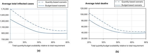
Figure 4 Sensitivity analysis on total resource availability (measured in terms of the total cost).

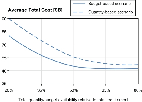
Table 6 Average number of regional outbreaks for both models

Model	Total resource availability
	20%	50%	80%
Quantity-based	1.89	1.44	1.38
Budget-based	1.63	1.33	1.20

As expected, the curves for all impact measures (average total number of infected, deaths, and total cost) exhibit a downward trend, for both allocation models, as the total resource availability increases. Increased total resource availability not only mediates a regional pandemic impact but also reduces the probability of spread to unaffected regions. For both models, as the resource availability approaches the resource requirement (starting from approximately 60%), the impact curves show a converging behavior, whereby the marginal utility of additional resource availability diminishes. This can be explained by noting that the total resource requirement was determined assuming the worst case scenario when all regions would be affected and provided with adequate resources to cover their respective populations at risk. It can also be observed that for all three measures, the budget-based model dominates the quantity-based model at all levels of resource availability. This can be attributed to the fact that the budget-based model, being less restrictive as having only one constraint (Section 1), also takes advantage of its ability to balance the relative cost and effectiveness of individual resources, such as vaccine, antiviral, etc. The difference in the performance of two models was as high as 339,079 infected cases, 19,724 fatalities, and 17.84 M in the pandemic cost (all attained at the 20% resource availability). The difference in policy performance gradually diminishes as the resource availability increases and as available quantities become close to be sufficient to cover the entire populations at risk in all regions: at 80% availability, the gap was 118,124 infected, 4,318 fatalities, and 5.07M in the pandemic cost.

Conclusions

Effective mitigation of influenza pandemics has to invariably rely on understanding of evolution of disease and population dynamics and intelligent resource allocation. As recently pointed by the IOM, the existing models fall short of providing dynamic decision support, which incorporates broader outcome measures including “costs and benefits of intervention”. In this paper, we present two large-scale simulation-based optimization models specifically aimed at addressing these challenges.

The models support development of dynamic predictive resource allocation strategies for a network of regional outbreaks. In both models, the underlying simulation mimics the disease and population dynamics of the affected regions. The quantity-based optimization model generates a progressive allocation of resource quantities, whereas the budget-based model aims at allocating the total resource budget. Both models seek to minimize the impact of ongoing and expected outbreaks. The impact measures incorporate morbidity, mortality, and social distancing, translated into the societal and economic costs of lost productivity and medical expenses. The models were calibrated using historic pandemic data and implemented on a sample cross-regional outbreak in Florida, with over 4M inhabitants.

Summary of the main results. We observed that for both models, the marginal utility of additional resource availability was steadily diminishing as the resource availability approached the resource requirement for a worst case scenario, in which all regions would be affected. We also showed that the quantity-based model was inferior to the budget-based model at different levels of resource availability. While the budget-based model includes the quantity-based solution as a special case, the former takes advantage of its inherent ability to balance the different relative cost and effectiveness of individual resources. Moreover, the budget-based model is less restrictive (the only constraint is the total available budget), and therefore, it has a richer geometry of feasible solutions at any decision epoch of pandemic evolution. The difference in model performance was particularly noticeable at lower levels of resource availability, which is in accordance with a higher marginal utility of additional availability at that levels. Hence, the budget-based model can be most useful in scenarios with very limited supply of resources.

Contributions of the model. The methodology presented in this paper is one of the first attempts to offer dynamic predictive decision support for pandemic mitigation, which incorporates measures of societal and economic impact. Our comparison study of the budget-based versus quantity-based progressive cross-regional resource allocations is also novel. In addition, our simulation model represents one of the first of its kind in considering a broader range of social behavioral aspects, including vaccination and antiviral treatment conformance. The simulation features a flexible design which can be particularized to a broader range of pharmaceutical and non-pharmaceutical interventions and more granular mixing groups.

Based on our methodology, we have also developed a decision-aid simulator with a GUI which is made freely available to general public through our web site at http://imse.eng.usf.edu/pandemics.aspx. The simulator allows the input of data for regional demographic and social dynamics, and disease related parameters. It is intended to assist public health decision makers in conducting customized what-if analysis for assessment of mitigation options and development of policy guidelines. Examples of such guidelines include targeted risk groups for vaccination and antiviral treatment, social distancing policies (eg, thresholds for declaration and lifting, closure options (ie, household-based, schools, etc.), and compliance targets), and guidelines for travel restrictions.

Limitations of the model. Lack of reliable data prevented us from considering geo-spatial aspects of mixing group formation in the testbed implementation. We also did not consider the impact of public education and use of personal protective measures (eg, face masks) on transmission, again due to a lack of effectiveness data.⁸³ We did not study the marginal effectiveness of individual resources due to a considerable uncertainty about the transmissibility of a future pandemic virus and efficacy of vaccine and antiviral. For the same reason, the vaccine and antiviral risk groups considered in the testbed can be adjusted, as different prioritization schemes have been suggested in the literature, based on predicted characteristics of a future virus. The form of social distancing implemented in the testbed can also be modified as a variety of schemes can be found in the literature, including geographical and social targeting. Effectiveness of these approaches is substantially influenced by the policy compliance, for which limited accurate data support exists. It will thus be vital to gather the most detailed data on the epidemiology of a new virus and the population dynamics early in the evolution of a pandemic, and to expeditiously analyze it to adjust the interventions accordingly.

Disclosure

The authors disclose no conflicts of interest.

References

- LonginiIMHalloranMENizamAYangYContaining Pandemic In uenza with Antiviral AgentsAm J Epidemiol200415962363315033640
- Centers for Disease Control and Prevention (CDC)Avian in uenza: Current H5N1 situation http://www.cdc.gov/flu/avian/outbreaks/current.htm#clusters2008 Last accessed on 02/09/2008.
- World Health Organization (WHO)Cumulative number of confirmed human cases of Avian In uenza A(H5N1) reported to WHO http://www.who.int/csr/disease/avian_influenza/country/cases_table_2010_03_04/en/index.html2010 Last accessed on 03/04/2010.
- World Health OrganizationPandemic (H1N1) 2010 - update 90 http://www.who.int/csr/don/2010_03_05/en/index.html2010 Last accessed on 03/04/2010.
- Arthur SchoenstadtSpanish Flu http://flu.emedtv.com/spanish-flu/spanish-flu.html2009 Last accessed on 12/15/2009.
- FedsonDSHantSPandemic in uenza and the global vaccine supplyClin Infect Dis2003361552156112802755
- AuninsJGLeeALVolkinDBVaccine productionBoca RatonCRC Press LLC2 ed2000
- World Health OrganizationPandemic (H1N1) 2009 vaccine deployment update -17 December 2009 http://www.who.int/csr/disease/swineflu/vaccines/h1n1_vaccination_deployment_update_20091217.pdf2009
- WHO Global Influenza ProgrammePandemic In uenza Preparedness and Response tech. rep.World Health Organization2009
- Centers for Disease Control and Prevention (CDC)Preparing for Pandemic Influenza http://www.cdc.gov/flu/pandemic/preparedness.htm2007 Last accessed on 04/27/2009.
- US Department of Health & Human ServicesHHS pandemic in uenza plan http://www.hhs.gov/pandemicflu/plan/2007. Last accessed on 03/27/2009.
- HandelALonginiIAntiaRTowards a quantitative understanding of the within-host dynamics of in uenza A infectionsEpidemics2009118519520161493
- PourbohloulBAhuedADavoudiBInitial human transmission dynamics of the pandemic (H1N1) 2009 virus in North AmericaInfluenza Other Respi Viruses2009321522219702583
- AtkinsonMWeinLQuantifying the Routes of Transmission for Pandemic InfluenzaBull Math Biol20087082086718278533
- PitzerVEOlsenSJBergstromCTDowellSFLipsitchMLittle evidence for genetic susceptibility to in uenza A (H5N1) from family clustering dataEmerg Infect Dis2007131074107618214184
- PitzerVELeungGMLipsitchMEstimating variability in the transmission of severe acute respiratory syndrome to household contacts in Hong Kong, ChinaAm J Epidemiol200716635535917493952
- YangYSugimotoJDHalloranMEThe transmissibility and control of pandemic in uenza A (H1N1) virusScience200932672973319745114
- YangYHalloranMESugimotoJLonginiIMJrDetecting human-to-human transmission of avian in uenza A (H5N1)Emerg Infect Dis2007131348135318252106
- CauchemezSCarratFViboudCValleronABoellePA Bayesian (MCMC) approach to study transmission of in uenza: application to household longitudinal dataStatist Med20042334693487
- ColizzaVBarratABarthelemyMVespignaniAThe role of the airline transportation network in the prediction and predictability of global epidemicsProc Natl Acad Sci U S A20061032015202016461461
- EpsteinJMParkerJCummingsDHammondRACoupled contagion dynamics of fear and disease: mathematical and computational explorationsPLoS One20083
- EpsteinJMGoedeckeDMYuFMorrisRJWagenerDKBobashevGVControlling pandemic flu: the value of international air travel restrictionsPLoS One20072
- HalloranMEInvited commentary: Challenges of using contact data to understand acute respiratory disease transmissionAm J Epidemiol200616494516968867
- ScharfsteinDOHalloranMEChuHDanielsMJOn estimation of vaccine efficacy using validation samples with selection biasBiostatistics2006761516556610
- GlassRBeyelerWMinHTargeted social distancing design for pandemic influenzaEmerg Infect Dis2006121671168117283616
- LipsitchMCohenTMurrayMLevinBRAntiviral resistance and the control of pandemic influenzaPLoS Medicine20074111115
- Nigmatulina KarimaRLarson RichardCLiving with influenza: Impacts of government imposed and voluntarily selected interventionsEur J Oper Res2009195613627
- WuJTRileySFraserCLeungGReducing the impact of the Next influenza pandemic using household-Based public health interventionsPLoS Med2006315321540
- MillsCRobinsJLipsitchMTransmissibility of 1918 pandemic influenzaNature200443290490615602562
- PatelRLonginiIHalloranMFinding optimal vaccination strategies for pandemic in uenza using genetic algorithmsJ Theor Biol200523420121215757679
- ColizzaVBarratABarthelemyMValleronAVespignaniAModeling the worldwide spread of pandemic influenza: baseline case and containment interventionsPLOS Medicine2007495110
- CooleyPGanapathiLGhneimGHolmbergSWheatonWHollingsworthCUsing influenza-like illness data to reconstruct an influenza outbreakMath Comput Model200892993919122846
- National Institute of General Medical SciencesModels of Infectious Disease Agent Study http://www.nigms.nih.gov/Initiatives/MIDAS/2008. Last accessed on 09/10/2008.
- FergusonNMCummingsDCauchemezSStrategies for containing an emerging influenza pandemic in Southeast AsiaNature200543720921416079797
- LonginiIMNizamAShufuXContaining Pandemic Influenza at the SourceScience20053091083108716079251
- FergusonNCummingsDAFraserCCajkaJPhilip CooleyCBurkeDSStrategies for mitigating an influenza pandemicNature200644244845216642006
- GermannTKadauKLonginiIMMackenCMitigation strategies for pandemic influenza in the United StatesProc Natl Acad Sci U S A20061035935594016585506
- EubankSGucluHKumarVModelling disease outbreaks in realistic urban social networksNature200442918018415141212
- HalloranMEFergusonNMEubankSLonginiIModeling targeted layered containment of an influenza pandemic in the United StatesProc Natl Acad Sci U S A20081054639464418332436
- MIDAS Report from the Models of Infectious Disease Agent Study (MIDAS) Steering Committee http://www.nigms.nih.gov/News/Reports/midas_steering_050404.htm2004 Last accessed on 09/10/2008.
- Committee on Modeling Community Containment for Pandemic InfluenzaModeling community containment for pandemic influenza: A letter report http://www.nap.edu/catalog/11800.html2006 Last accessed on 12/09/2008.
- Centers for Disease Control and Prevention (CDC)Interim pre-pandemic planning guidance: Community strategy for pandemic influenza mitigation in the United States http://www.pandemicflu.gov/plan/community/community_mitigation.pdf2007 Last accessed on 04/01/2009.
- DasTSavachkinAA large scale simulation model for assessment of societal risk and development of dynamic mitigation strategiesIIE Transactions200840893905
- MeltzerMCoxNFukudaKThe economic impact of pandemic influenza in the United States: Priorities for interventionEmerg Infect Dis1999565967110511522
- WuJTRileySLeungGSpatial considerations for the allocation of pre-pandemic influenza vaccination in the United StatesProc Biol Sci20072742811281717785273
- LawlessJFLawlessJFStatistical models and methods for lifetime dataNew YorkWiley1982
- DiekmannOHeesterbeekJAPMathematical epidemiology of infectious diseases: Model building, analysis and interpretationNew YorkWiley2000
- BrundageJFShanksGDDeaths from bacterial pneumonia during 1918–19 influenza pandemicEmerg Infect Dis200814119318680641
- Centers for Disease Control and Prevention (CDC)CDC influenza operational plan http://www.cdc.gov/flu/pandemic/cdcplan.htm2006 Last accessed on 03/27/2009.
- PasteurSInfluenza A(H1N1) 2009 Monovalent Vaccine http://www.fda.gov/downloads/biologicsbloodvaccines/vaccines/approvedproducts/ucm182404.pfd2009 Last accessed on 11/18/2009.
- BlendonRJKooninLMBensonJMPublic response to community mitigation measures for pandemic influenzaEmerg Infect Dis20081477818439361
- SadiqueMZEdmundsWJSmithRDPrecautionary behavior in response to perceived threat of pandemic influenzaEmerg Infect Dis200713130718252100
- MaunderRHunterJVincentLThe immediate psychological and occupational impact of the 2003 SARS outbreak in a teaching hospitalCan Med Assoc J20031681245125112743065
- RobertsonEHershenfieldKGraceSLStewartDEThe psychosocial effects of being quarantined following exposure to SARS: a qualitative study of Toronto health care workersCan J Psychiatry20044940340715283537
- PearsonMLBridgesCBHarperSAInfluenza vaccination of health-care personnel Recommendations of the Healthcare Infection Control Practices Advisory Committee (HICPAC) and the Advisory Committee on Immunization Practices (ACIP)[Internet].2006 Last accessed on 10/28/2009.
- KeaneMWalterMPatelBConfidence in vaccination: a parent modelVaccine2005232486249315752835
- NiederhauserVPBaruffiGHeckRParental decision-making for the varicella vaccineJ Pediatr Health Care20011523624311562641
- RhodesSDHergenratherKCExploring hepatitis B vaccination acceptance among young men who have sex with men: facilitators and barriersPrev Med20023512813412200097
- RosenthalSLKottenhahnRKBiroFMSuccopPAHepatitis B vaccine acceptance among adolescents and their parentsJ Adolesc Health1995172482558580126
- SmailbegovicMLaingGBedfordHWhy do parents decide against immunization? The effect of health beliefs and health professionalsChild Care Health Dev20032930312823336
- Colardo Department of Human Services Division of Mental HealthPandemic influenza: Quarantine, isolation and social distancing http://www.flu.gov/news/colorado_toolbox.pdf2009 Last accessed on 10/28/2009.
- SafranekTJLawrenceDNKuriandLTReassessment of the association between Guillain-Barré syndrome and receipt of swine influenza vaccine in 1976–1977: results of a two-state studyJ Epidemiol1991133940
- CummingsKMJetteAMBrockBMHaefnerDPPsychosocial determinants of immunization behavior in a swine influenza campaignMed Care197917639649221759
- The New YorkerThe fear factor http://www.newyorker.com/talk/comment/2009/10/12/091012taco_talk_specter2009 Last accessed on 10/28/2009.
- The New York TimesDoctors swamped by swine flu vaccine fears http://www.msnbc.msn.com/id/33179695/ns/health-swine_flu/.2009 Last accessed on 10/28/2009.
- GosaviADasTKSarkarSA simulation based learning automata framework for solving semi-Markov decision problems under long run average rewardIIE Transactions in Operations Engineering200136557567
- SavachkinAUribe-SánchezADasTPrietoDSantanaAMartinezDSupplemental data and model parameter values for cross-regional simulation-based optimization testbed http://imse.eng.usf.edu/pandemic/supplement.pdf2010 Last accessed on 04/15/2010.
- U.S Census Bureau2001American community survey http://www.census.gov/prod/2001pubs/statab/sec01.pdf2000 Last accessed on 03/27/2009.
- Bureau of transportation statistics2001 National household travel survey (NTHS) http://www.bts.gov/programs/national_household_travel_survey/.2002 Last accessed on 12/09/2008.
- Tampa International Airport Daily Schedule http://www.tampaairport.com/.2008 Last accessed on 12/09/2008.
- Miami International Airport http://www.miami-airport.com/. Last accessed on 12/09/2008.
- Jacksonville Aviation AuthorityDaily Schedule http://www.jaa.aero/General/Default.aspx2008 Last accessed on 12/09/2008.
- Tallahassee Regional AirportDaily Schedule http://www.talgov.com/airport/index.cfm2008 Last accessed on 12/09/2008.
- Writing committee of the World Health Organization (WHO)Consultation on human influenza A/H5. Avian influenza A(H5N1) infection in humansN Engl J Med20053531374138516192482
- World Health Organization (WHO)WHO guidelines on the use of vaccine and antivirals during influenza pandemics http://www.who.int/csr/resources/publications/influenza/11_29_01_A.pdf2004 Retreived 03/27/2009.
- Institute of Medicine (IOM)Antivirals for pandemic influenza: Guidance on developing a distribution and dispensing programThe National Academies Press2008 Academies Press.. 2008.
- TreanorJCampbellJZangwillKRoweTWolffMSafety and immunogenicity of an inactivated subvirion influenza A(H5N1) vaccineN Engl J Med20063554134316571878
- BlendonRJDesRochesCMCetronMSBensonJMMeinhardtTPollardWAttitudes toward the use of quarantine in a public health emergency in four countriesHealth Aff2006251525
- PayScaleJob: Registered Nurse (RN) http://www.payscale.com/rcsearch.aspx?country=US&str=Registered+Nurse+. Last accessed on 12/28/2009.
- Centers for Disease Control and PreventionCDC vaccine price llist http://www.cdc.gov/vaccines/programs/vfc/cdc-vac-price-list.htm#flu. Last accessed on 12/28/2009.
- PharmacyChecker.comPricing & ordering comparisons http://www.pharmacychecker.com/Pricing.asp?DrugId=36260&DrugStrengthId=61300&sortby=Price. Last accessed on 12/28/2009.
- HalfhillTInflation Calculator http://www.halfhill.com/inflatation.html2009 Last accessed on 12/04/2009.
- BellDMNon-pharmaceutical interventions for pandemic influenza, national and community measuresEmerg Infect Dis2006128816494723