An Epigenetic Pacemaker is Detected Via a Fast Conditional Expectation Maximization Algorithm

Abstract

Aim: DNA methylation has proven to be a remarkably accurate biomarker for human age, allowing the prediction of chronological age to within a couple of years. Recently, we proposed that the Universal PaceMaker (UPM), a flexible paradigm for modeling evolution, could be applied to epigenetic aging. Nevertheless, application to real data was restricted to small datasets for technical limitations. Materials & methods: We partition the set of variables into to two subsets and optimize the likelihood function on each set separately. This yields an extremely efficient Conditional Expectation Maximization algorithm, alternating between the two sets while increasing the overall likelihood. Results: Using the technique, we could reanalyze datasets of larger magnitude and show significant advantage to the UPM approach. Conclusion: The UPM more faithfully models epigenetic aging than the time linear approach while methylated sites accelerate and decelerate jointly.

Keywords::

• conditional expectation maximization
• DNA methylation
• universal pacemaker

DNA methylation is a well-studied epigenetic mark that functions to define the states of cells as they undergo developmental changes [16]. Beyond changes during development, methylation also undergoes systematic changes in humans as they age [3,11,14,20]. Therefore, DNA methylation serves as a central epigenetic mechanism that helps define and maintain the state of cells during the entire life cycle [1,2,9]. In order to measure genome-wide levels of DNA methylation, techniques such as bisulfite sequencing and DNA methylation arrays are used [12].

The first description of a robust epigenetic clock that worked across different tissues was presented by Steve Horvath [7]. The clock consists of 353 CpG sites, whose weighted sum yields an estimate of chronological age to within a couple of years. The clock also log transforms the ages if individuals are less than 20 years old, while keeping those greater than 20 untransformed. The time linearity, at least for adults of age greater than 20 years, of the Horvath clock makes it the ‘epigenetic parallel’ of the classical evolutionary version of the molecular clock (MC) [23,22].

In a recent work [18], we have adapted mechanisms from molecular evolution to the process of methylation. Specifically, we have used the Universal PaceMaker (UPM or simply pacemaker – PM) of genome evolution [15,17,19,21] to allow for rate variability as opposed to the constancy imposed by the MC concept. In the UPM approach, we assume that all sites are changing linearly with an adjusted time, which is a nonlinear function of the chronological time. When replacing genes with CpG sites and interpreting UPM rate increases as accelerated aging, the UPM framework becomes an appealing paradigm to study age-related changes in DNA methylation.

In this work, we propose a conditional expectation maximization (CEM) algorithm [13] that extends the classical EM algorithm [4] by partitioning the parameter set into several parts when optimizing the likelihood function over the entire set simultaneously is hard. The choice of partitioning is important as it determines the optimization algorithm. The partitioning we used here uses two fast optimization algorithms. In the first – the site step – we use the same parameters as used by the linear (MC) model that leads to a linear algebra solution in [19]. We also mention a simple, direct solution, relying on the special structure of the UPM (whose details are deferred to a separate publication). The latter allows us to bypass the heavy linear algebra step completely, yielding a significant practical and asymptotic reduction in both time and space. This reduction is complemented by a fast solution to the second step, the time step, of the CEM. This yields a very fast algorithm that terminates in few iterations of the EM algorithm.

These improvements enable us to increase substantially the scale of inputs analyzed by the method, allowing us to infer the structural properties of the framework, such as false positives and negatives. In the part analyzing real biological data, we revisit our previous results from DNA methylation data coming from human blood [6] that we previously analyzed in [18]. It allows us to quantify the effective gain provided by the improved algorithm not only in terms of the quantity of data processed but also in the types of biological insights we are able to generate from the results. The current analysis achieves improvements in several parameters, but most significantly in the reduction of the average variance per term in the likelihood function by a factor of almost two. We also analyzed two other human datasets that have not been analyzed under the UPM framework before. Both datasets are much larger than the sizes handled before; furthermore, they come from two different tissues as opposed to the single tissue in [18]. Their analysis under the UPM demonstrated significant improvement in the model t to the data, by tens of percentages. These results, along with the substantially larger inputs analyzed, both in number of individuals and methylation sites, strengthen our preliminary observations from our previous pilot work, suggesting that the UPM framework models epigenetic aging better than the MC, by allowing all sites to accelerate and decelerate jointly, accounting for nonlinear trends in aging.

Materials & methods

The evolutionary models

In our model, we have m individuals and n methylation sites in a genome (or simply sites). The ages of each individual form a set t of time periods {t_j} corresponding to each individual j’s age. There is additionally a set of sites s_i that undergo methylation changes, where the rate of site i is r_i. The methylation at sites starts at some initial level at birth $S_i^0$. Henceforth, we will index sites with i and individuals with j. Therefore, the variables associated with a site, r_i and $S_i^0$are kept in the vectors of size n and the variables associated with individuals, t_j are kept in a vector t of size m.

s_i,j measures the methylation level at site s_i in individual j at time t_j. Under the MC model (i.e., when rate is constant over time), we expect: s_ij = $S_i^0$ + r_it_j. However, we have noise ε_i,j that is added and therefore the observed value ŝ_ij is ŝ_ij = $S_i^0$ + r_it_j+ ε_i,j. Given the input matrix Ŝ = [ŝ_i,j], holding the observed methylation level at site s_i of individual j, the goal is to find the maximum likelihood (ML) values for the variables r_i and $S_i^0$ for 1 ≤i ≤n. Henceforth, we define a statistical model under which ε_i,j is assumed to be normally distributed, ε_i,_j ∼ N(0,σ²). In [18], we showed that minimizing the following function, denoted residual sum of squares (or RSS), is equivalent to maximizing the model’s likelihood:Equation 1

We also showed that there is an efficient and precise linear algebra solution to this problem that we describe in more detail below.

In contrast to the MC, under the UPM model, sites may arbitrarily and independently of their counterparts in other individuals, change their rate at any point in life. However, when this happens, all sites of that individual change their rate proportionally such that the ratio r_i/r_i′ is constant between any two sites i, i′ at any individual j and at all times.

In [18], we showed that this is equivalent to extending individual j’s age by the same proportion of the rate change. The new age is denoted as the epigenetic age (e-age) in contrast to the chronological age (c-age). Therefore, here we do not just use the given c-age but estimate the e-age of each individual. Hence, under the UPM we must find the optimal values of $S_i^0$, r_i, and t_j (where t_j represents a weighted average of the rate changes an individual has undergone through life). We describe below the solution to this optimization problem. We note that the deviation between the chronological age and the estimated epigenetic age is an age difference which, when positive, is denoted as age acceleration and deceleration otherwise.

To compare between the two models, MC and UPM, we show that under our statistical setting we can use standard tools as follows. Under the MC model, a constant rate of methylation at each site is assumed. This induces linearity with time which is the individual’s age. Alternatively, in the competing, relaxed model (UPM), no such restriction exists, and in turn an ‘epigenetic’ age for each individual is estimated. By this definition, the ML solution under the relaxed model cannot be worse than the constrained model as the MC is contained, as a special case, in it. Therefore, in order to compare the approaches, we use the likelihood ratio test (LRT) as explained next.

Likelihood ratio test

The LRT is a statistical test used to compare the goodness of fit of two competing models, one of which (the null model) is a special case of the other, more general, one. The log of the ratio of the two likelihood scores distributes as a χ² statistic and therefore can be used to calculate a p-value. This p-value is used to reject the null model in the conventional manner. Specifically, let Λ = L₀/L₁ where L₀ and L₁ are the ML values under the restricted and the more general models, respectively. Then asymptotically, -2 log(Λ) will distribute as χ² with degrees of freedom equal the number of parameters that are lost (or fixed) under the restricted model.

In our case, it is easy to see thatEquation 2

where and are the ML values for RSS under MC and PM, respectively. Hence, we set our χ² statistic asEquation 3

Algorithm

The heart of the technical improvement is a CEM algorithm. We first give a brief overview of the EM algorithm and then specialize to CEM. The EM algorithm is a statistical, model-based algorithm, designated to optimize a missing-data function where an efficient solution is not at hand [1]. It operates iteratively in order to reach a local maximum point. In each iteration, ‘guessed values’ to the hidden variables are assumed. Then, at the expectation step, with these guessed values all data are completed and expected values to the hidden variables can be computed. Then, at the maximization step, the expected values become the next variables’ guessed values, and a new iteration starts. As the expectation step concerns with integrating over all parameter spaces, and such integration can be computationally costly, the CEM algorithm breaks the parameter set into two subsets, and optimizes separately each subset [13].

We now provide a description of the main technical result of this work that is a significant improvement of the previous standard linear algebra solution used in [18]. This component comprises one of the two building blocks of the high-level CEM algorithm and therefore we describe it first.

Solving the MC model

In order to solve the MC model, we need to minimize the RSS. It can readily be shown that maximizing the likelihood function L is equivalent to minimizing the RSS. Under the general case, there is no efficient (polynomial time) solution to this problem, let alone a closed form, and therefore this task is normally done by some numerical method.

In our case, however, the special structure of the problem allows a more efficient solution. When the residuals are linear in all unknowns, a solution can be found using linear algebra tools that have a closed-form solution (given that the columns of the matrix are linearly independent). The goal is to formulate the task in a matrix form as we show below. Under this formalism, the optimal (ML) solution is given by the vector $\hat{\beta }$ as follows:Equation 4

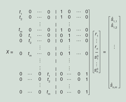
where X is a matrix over the variable’s coefficients in the problem, y is a vector holding the observed values – in our case the entries of Ŝ, and the RSS equation can be written such that for every row i in X, y_i−X_i,jβ_j is a component in the RSS. Recall that for m individuals and n sites, our RSS contains mn components each of which corresponds to an entry in Ŝ in the form ŝi,j₋t_jr_i-$S_i^0$ where ŝ_i,j and t_j are input parameters. This leads to the following observation (stated in [18]):

Observation 5.1 ([18]), let X be a mn × 2n matrix whose kth row corresponds to the (i,j) entry in S, the first n variables of β are the r_i’s and the second n variables are the $S_i^0$’s, and the im + j entry in y contains s_i,j (see Figure 1). Then, if we set the kth row in X all to zero except for t_j in the i’th entry of the first half and 1 in i’th entry of the second half, we obtain the desired system of linear equations (see again illustration for row setting in Figure 1).

Figure 1.  The mn × 2n matrix X that is used in our closed-form solution to the molecular clock case.

Every row corresponds to a component in the RSS polynomial and the corresponding entries (ith and i + nth) in that rows are set to t_j and 1, respectively.

RSS: Residual sum of square.

The likelihood score is calculated by plugging in the values obtained for $\hat{\beta }$ in Equation 4 to the likelihood function (or alternatively into the RSS).

A standard (algebraic) implementation of Equation 4Equation 4 is computationally demanding as it requires the multiplication of the huge 2n × nm matrix X, followed by inverting the product matrix, and then another multiplication. Luckily, the specific matrices handled in our case possess substantial structure that is imposed by the UPM framework. Therefore, by a series of improvements, whose details are fairly involved and beyond the scope of this work, we can obtain a fast, closed-form solution to Equation 4Equation 4 that entirely eliminates the heavy linear algebra machinery. This is done by a series of four stjpg, each eliminating an algebraic operation applied to an intermediate matrix, until the result is obtained. The final result is achieved by showing that the vector $\hat{\beta }$ from Equation 4 can be constructed directly without any of these operations. We here provide the outline of this construction.

• Solving the X^T X operation: We start with the matrix product X^T X. Recall our auxiliary matrix X described in Figure 1. This matrix is huge as it contains nm rows and 2n²m entries. However, not only it is very sparse, it is also very structured. We can, therefore, show that the product X^T X matrix of size 2n × 2n, is composed of four n × n square submatrices, and each of these submatrices is diagonal. This fact is the basis to the reduced computation along the whole process.

• Inverting the X^T X matrix: After we multiply X by itself, by Equation 4Equation 4 we need to invert the product. Here, we use identities from linear algebra regarding inverting block submatrices and the fact that all our block submatrices are diagonal and their values can be computed directly from the input without calculating the matrix product itself. This yields that the inverted matrix is also composed of four n × n diagonal matrices whose values can be computed directly from the input.

• Obtaining the (X^TX)^-1X^T matrix: The third step of our derivation is to multiply the matrix (X^T X)^-1 obtained in the previous step, with the transpose of the original matrix X. This matrix, although not square anymore, carries the structure of its two originating matrices and can be described as expanded diagonal matrix where each entry in the diagonal is duplicated a constant number of times. Moreover, as we did not have to compute its two originating matrices, we, therefore, need not to compute this matrix as well and can calculate the value of each entry of it directly from the input vector t holding each individual’s age – t_i.

• Finalizing: After settling the structure of the (X^T X)^-1X^T matrix, the final step is to derive the values of our variates, the n site rates and the n site starting states. This cannot be done in less than 2 nm operations as this is the number of our inputs – n states of each of the m individuals. However, the matrix (X^T X)^-1X^T has only m nonzero entries in each row and moreover, their exact location is known and their value is dependent only on that location. The latter implies that we do not need to hold the matrix or even some advanced data structure to keep sparse matrices. Instead, in each row k of (X^T X)^-1X^T we find the entries in y that are affected, we calculate the value in the matrix (this is determined solely by the indices of that entry) and perform the multiplication with the corresponding value in y. The above description yields that the result vector $\hat{\beta }$ from Equation 4Equation 4 can be computed directly without all the heavy linear algebra machinery.

Solving the UPM problem

In the previous part, we have provided a simple solution to the MC problem that does not rely on any linear algebraic operation. However, for the UPM problem, the least square problem is not linear since the set of times t_j’s also need to be estimated. Hence, the formulation from the step above is invalid and we are doomed to seek a heuristic solution that will provide a sound result in reasonable time and for nontrivial datasets. In [18], we have shown a simple algorithm that searches exhaustively the space of times (instead of the entire space of times, rates and starting states) and finds the optimal rates and starting states for each time set. Due to its limitations, we were limited to small datasets of at most a hundred individuals and three hundred sites, and much less than that (in sites) for simulation studies. We now show a CEM [13] algorithm for the same problem where the maximization step is subdivided into two stjpg in which at each step the likelihood function is maximized over a subset of the variates conditional on the values of the rest of the variates. As our set of variates under the UPM formulation is augmented with the times (individual’s epigenetic ages), it is now composed of the set of sites, starting states, site rates and times. Hence, in order to arrive at a local optimum point, we partition the set of variates into two: one is the set of rates and start states, and the other is the set of times. The underlying CEM algorithm optimizes separately each such set by alternating between two stjpg: the site step in which the site-specific parameters, rate and starting state, are optimized, and time step in which individual’s times are optimized. By the definition of the CEM, at every such step an increase in the likelihood is guaranteed, until a local optimum is reached.

In our specific case, it remains to show how we optimize the likelihood function at each step. Note that one of the sets of variates is exactly the set, we solved for under the MC formulation – the set of rates and site start states. For this set, we already have a very fast algorithm as we illustrated above that is provably correct by Equation 4Equation 4 . However, as opposed to [18] where we had the same partition over the variates, there, not only optimization of the times was done exhaustively but also once the optimal rates for given times were found, they were ignored in the subsequent optimization of the times. Here, every set is optimized based on the basis of the other set. This is what makes the current algorithm so fast.

We now show how maximization is done for the other set of variates – the set of times t_j. In the site step when we optimize the t_j’s, we treat all other variables of the RSS function (Equation 1Equation 1 ) as constants. Moreover, as can be perceived from the RSS, all t_js are mutually independent – they do not appear jointly in any term in the RSS. That means we can optimize them separately by an expression in the other variables that appear as constants.

The complete CEM–UPM algorithm

For completeness here, we describe the full high-level CEM algorithm that alternates between the two stjpg, the time step and the site step as long as an improvement greater than a threshold δ_CEM is attained. We use RSS(p) to denote the evaluation of the polynomial RSS with a set of parameters p.

Procedure CEM UPM (Ŝ, δ_CEM):

1.	Toss a random m-dimension vector t;
2.	Toss two random n-dimension vectors s0, r;
3.	Let y be a mn-dimension vector holding the entries of Ŝ from top down, left to right (i.e., yim+j ← ŝi,j);
4.	(r‘, s′0) ← apply the site step with parameters t and y;
5.	t′ ← apply the time step with parameters r‘, s‘0 and y;
6.	RSS 0 ← RSS(Ŝ, t, s0, r);
7.	RSS 1 ← RSS(Ŝ, t′, s‘0, r′);
8.	if RSS1 – RSS0 > δCEM: (t, s0, r) ←(t′, s‘0, r‘); return to 4.

We conclude by noting that the algorithm in [18] also operates in the two spaces as here – the time space and the site step. However, as opposed to the CEM UPM above, in [18], optimization was done only in the time space and the site space was inferred manually by us and hence was hidden from the optimization algorithm. This difference is principal and was proved crucial in minimizing the hill-climbing stjpg, and hence for the speed up of the CEM UPM algorithm.

Implementation

Simulation results

In order to measure the properties of the new algorithms under controlled conditions, we conducted the following simulation study. We start with an overview elucidating the underlying ideas and goals behind this section. Recall that the decision whether a UPM is in effect or not is made by refuting the null hypothesis which assumes no UPM, or in other words, the existence of an MC, which implies time linearity. This decision is made by computing the LRT and using the χ² distribution, which returns the cumulative probability for that χ². This in turn can be contrasted to a supplied threshold in order to refute MC or not.

The parameters we vary along the runs are these: the UPM variance that affects the intensity of the UPM and determines the e-age or equivalently, how much an individual deviates from its c-age, and the noise variance that is how much each site i of that individual j deviates from its expected methylation state as defined by ŝ_ij = $S_i^0$ + r_it_j + ε_i,j. Naturally, the bigger that variance of ε_i,j, the more noisy is the signal and the harder it is for the algorithm to detect the UPM (if such indeed exists). We also measure the effect of the number of individuals and number of sites as these constitute (but each differently) the number of samples we observe from the underlying generative model. Naturally, we expect the larger the sample size, the better the identification. The focus, however, is on the effect of each parameter.

The measured quantity is the cumulative probability returned by the χ². For the sake of simplicity, we denote it in the figures depicting this study as a p-value (although this p-value is obtained by subtracting this quantity from 1). While this is not exactly the success rate, it provides more insight to the method’s performance and can easily be translated to a success rate.

All experiments, simulation and real data, were done on a Mac laptop with a 2.7 GHz Intel Core i5 processor with 8GB memory.

Our first study is basically the same as was carried out in our previous work [18], however, with the improved algorithm we are able to conduct experiments of substantially larger scale (500 and 1000 individuals here vs 50 and 100 in [18]). This increase in magnitude allows us to derive conclusions about false-negative and -positive rates. The graphs depicting our simulation results are found in Figure 2 in the text. The false-negative rate of a method is defined as the rate at which a method fails to detect an existing event or signal. In our case, we measured how well the algorithm detects an existing UPM under various conditions. Therefore, in all experiments a UPM is in effect (although with different magnitudes). As mentioned above, the measured quantity is the cumulative probability that is returned from the χ² function (see ‘Materials & methods’ section which describes how this is computed in this case), which, in turn, can be used to refute the null hypothesis (no UPM) at any desired threshold (e.g., 0.95, 0.99). The parameters to the model are as follows: the variance of the PM, in other words, how much the individuals vary their epigenetic age (e-age) from their chronological age (c-age). Specifically, for individual j with c-age t_j, we set its e-age e_j as e_j = t_j + ε_j where ε_j ∼ N(0,σ_PM) and σ_PM is the PM variance. Therefore, the bigger σ_PM, the farther e_j from t_j and we get a stronger UPM effect.

Figure 2.  Human blood data results.

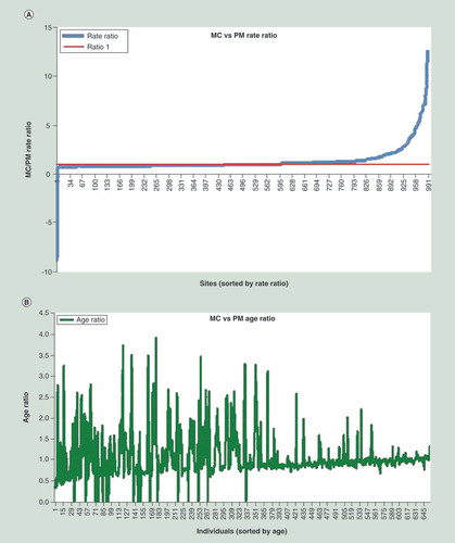
(A) Rate acceleration/deceleration under PM versus MC: curve indicates the MC/PM rates, respectively, at each site in the study. As can be seen, rates generally maintain their original sign under both MC and PM, however, some sites accelerate and others decelerate. (B) Age acceleration/deceleration under PM versus MC: ages were sorted in ascending sequence. For every time, the ratio between the PM-inferred time to real chronological time is plotted.

MC: Molecular clock; PM: Pacemaker.

The noise variance, determining how much each site of an individual deviates from its expected epigenetic state (see Var[ε_i,j] in the preliminaries). Finally, as our improvement allows us to increase sample size, we measured the returned p-value as a function of the number of sites. The intention in this part goes beyond showing more or less successful identification of the PM (due to high or low p-value, respectively), rather to show how the various parameters of the system, such as number of sites, the prominence of the UPM, affect the system’s response.

First (see Figure 2A), both the number of sites and the number of individuals are fixed at 1000 for both curves, but the PM variance (σ_PM – the tendency of epigenetic age to vary from MC age) differs. It is shown that under PM variance 0.15 a very high p-value (practically 1) is returned by the LRT and hence, the UPM is always inferred by the method, for every site noise Var[ε_i,j]. For PM variance 0.05, under moderate site noise, we also obtain high p-values, sufficient for accurate PM identification rates as well. Next (see Figure 2B), the effect of site variance (noise) is examined again, but under two numbers of sites. The PM variance is small in both tests -0.05. It is shown that under moderate site noise, we obtain high p-values under both number of sites, however, as the noise increases, we start to see a difference in performance.

Next, rates of false positives, defined here as the returned p-value when no real UPM is in effect, under several parameter combinations are checked. Recall that the PM signal is merely its variance σ_PM that causes individuals to develop their own rate and deviate from their chronological age. In the previous part, the false-negative rate was studied and, therefore, PM was always in effect and we checked how well the system detects it. Here, however, we set σ_PM = 0 (i.e., no PM) and test false detection of PM (through the returned p-value). For this purpose, we had to increase substantially the noise – site variance Var[ε_i,j] – and it ranges now from 10 to 90 (as opposed to 1–8 before). Such a high noise level may mislead the procedure to infer falsely PM. Graphical representations of these results are shown in Figure 3. We study three numbers of individuals -10, 50 and 200. In each case, four numbers of sites are examined and as expected, the larger this number is, the smaller the false positive (FP) rate. Nevertheless, under tiny and unrealistically small numbers of individuals 10, the FP rate is very high (but again, with a very strong noise level). However, under reasonable numbers on individuals 200, and in particular 200 sites, the FP rate decreases to 10% (and again, the model still includes very high noise).

Concluding this part, the two studies above (summarized in Figures 2 & 3), show that when using large enough numbers of sites and individuals, both the false negarive and FP rates drop to manageable levels, and provide reliable results.

Figure 3.  E-age versus c-age scatter plots.

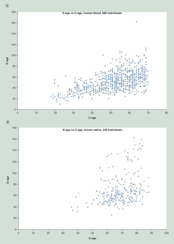
Scatter plots of epigenetic age versus chronological age demonstrating the deviation of each individual from the linear correlation. (A) The GSE42861 human blood dataset: 1000 most informative sites of 689 individuals. Analysis provided 19% increase in explanation (decrease in the variance). (B) The GSE78874 human saliva dataset: 3000 most informative sites of 259 individuals. Analysis provided 50% increase in explanation.

Reanalysis of human blood data

We now report on our results applying our CEM–UPM algorithm to methylation data from blood previously reported in [6]. The data were collected using the Illumina 450 K DNA methylation array platform.

The resulting data matrix contains about 450,000 CpG sites measured across 656 human individuals. In order to limit ourselves to a manageable size, we chose the 1000 sites providing the most signal by exhibiting the largest variance. We note that we have already analyzed the same dataset in [18], however, on a much smaller sample size (both number of individuals and sites). This reanalysis enables us to demonstrate the contribution of the algorithmic improvement provided here.

Result analysis

We applied both models to the human blood sample reported in [6] – the MC via the linear algebra step constrained to chronological ages, and the UPM via the CEM–UPM algorithm. For MC, we obtained RSS_MC = 50769.81, while for the UPM we obtained RSS_UPM = 48918.42. These two results by the LRT formula 3 (see Materials & methods section) yield χ² = 24369.06. As we have additional 656 free variables (the times t_j’s), we can calculate p-value with this as our degree of freedom that is practically 1. Nevertheless, we can use more informative indicators in order to measure the improvement attained by using much larger samples compared with [18]. While in [18], an increase in the average log likelihood under the UPM was of 2%, here, the increase in the average log likelihood under the UPM was of 3.7%, an improvement of almost twice. The improvement in χ² is from 3517 to 24,369.06 (although here we have significantly more free variables, so the results are not strictly comparable). It is important to note that while these improvements seem small, they are obtained over many terms (thousands in the previous approach and more than half a million now), and hence yielding a cumulative probability practically equal to 1 (or p-value zero).

Next, we analyzed the biological meaning of our new results. The prime output of the algorithm is the RSS that should be minimized in order to maximize the likelihood of the model. Nevertheless, recall that the procedure, in addition to the RSS, also estimates new rates and epigenetic ages. While we cannot guarantee that these are the optimal values (such as those attained at the global ML point), our experiments suggest that these are not very far from them and some general trends can be inferred. Figure 2A and B depicts two general trends that emerge from our results. In the left (Figure 2A), we show for each site, the ratio between its MC to PM rate, where the sites are sorted by that ratio (increasing order). First, we see that apart from very few sites on the left, most of the sites kept their direction under both models. Most of the sites (568 out of 1000) have increased their rate under UPM, a result that complies with our age observation as we now describe.

In the right (Figure 2B), we show the ratio between MC (chronological) and PM age, for every individual in the study. Individuals are ordered by their chronological age. Individual (a point on the x-axis) whose y value is greater than 1 accelerated her/his age and vice versa. Such a presentation allows us to examine the hypothesis of whether a general trend in the population exists, or epigenetic age acceleration/deceleration is personal and erratic.

The trend we set to test is whether, in general, the rate acceleration is more pronounced at younger versus older ages, as was suggested by previous studies [7]. The latter implies a monotonic increase in the ratio of MC versus UPM with respect to age. Figure 2B indeed shows a steady increase from a ratio of around 0.5 to around 1. We note that due to the strong noise, we cannot point to a strict monotonic increase, however, the trend is evidently noticed. Moreover, while the same trend was shown in our study in [18], here, it is demonstrated over a much larger dataset (656 individuals vs 100) and is substantially more steady.

Additional datasets

To further demonstrate the performance of the new algorithm, we applied it to two more human datasets. One of these two contains even more individuals than the one analyzed before, 689 individuals, and the other has less individuals – only 259 – but significantly more sites − 3000.

We first applied the CEM UPM algorithm to the blood dataset of 689 individuals [10]. Running time was 2:01 min. The total MC RSS score (error) was 1135.75 versus total UPM RSS of 806.03. This, in turn, yields a χ²: 236,274.73 that with degree of freedom (DF) 689 gives a p-value practically 1, refuting outright the MC hypothesis. The average MC error per term was 0.0406 and the average UPM error per term was 0.0342, yielding an improvement of 18.7%.

The second dataset was from human saliva [8]. This dataset contains methylation data over 259 individuals with age ranging from 36 to 88. To demonstrate the power of the method, we took the 3000 sites of this dataset, maximizing the covariance with age. Running time for this dataset was 09:26 min. Total error under MC was 3695.53 versus 1643.50 under UPM, yielding χ² of 629,597.05 that with DF 259 gives practically p-value 1 as in the former datasets. However, here the reduction in noise per term was very dramatic, from 0.0689 under MC to 0.0459 under UPM, an impressive improvement of 50% in the variance.

In Figure 3, we show another interpretation of the results. Here, the graphs are scatter plots of the e-age (y-axis) versus c-age (x-axis). In Figure 3A, we see the results for the 689 individuals’ blood data and in Figure 3B, for the 259 individuals’ saliva data. These graphs show the deviation of individuals’ e-age from their c-age. While under MC, we would expect e-age to be linearly correlated with c-age, here in both data we see significant deviations from any linearity, explaining the difference we observe in the variance for these two additional datasets.

Conclusion & future perspective

In this work, we devised a CEM algorithm to the problem of inferring epigenetic pacemaker that we name CEM–UPM. The mathematical definition of the problem, as well as a standard algorithm was provided by us in a previous work, however, the improvements provided here enable us to analyze inputs, both synthetic and biological, of significantly larger sizes. The improvements rely on speeding up the two maximization stjpg of the CEM. In the principal, the site step, the heavy linear algebra machinery is completely replaced by a manual derivation of optimal values of the model parameters, yielding an asymptotic saving in both run time and space by the major factor of the number of sites. In the secondary, the time step, the UPM structure allows for linear closed-form solution of the likelihood function.

These improvements, in turn, lead to conclusions regarding properties of the method such as error rates that could not have been drawn using the previous algorithm that could analyze substantially smaller inputs. In the real-data realm, we both reanalyzed the human blood dataset we analyzed in [18], and two new datasets, analyzed for the first time under the UPM framework. The reanalysis of the human blood allows us to quantify the improvement achieved by the algorithmic improvement in terms of real data. Specifically, we obtained an increase of almost twice in the correlation coefficient RSS² compared with [18] over the same dataset (but averaged over an order of magnitude more terms in the likelihood function). The two new datasets are of even larger size than the first human blood dataset. In these, although we have no record of previous analysis under the UPM framework, the improvement in the variance with respect to MC is very significant (with up to 50% in the second), leaving no doubt about the existence of a UPM in human aging.

Finally and importantly, the use of advanced tools such as symbolic algebra has value beyond the mere algorithmic improvements illustrated here, rather it grants a deeper understanding of the internals of the model that cannot be achieved otherwise. As a future research direction, we seek to further understand the likelihood surface. This understanding will not only teach us about the degeneracy of this surface with regard to multiple ML points but also the relationship between them and what invariants they satisfy. In the biological realm, an immediate goal is to provide a rigorous analysis of the trends we see in aging – is there a trend in the population toward nonlinear (i.e., constant) ratio between epigenetic age versus chronological age.

Summary points

• DNA methylation is a well-studied epigenetic mark that functions to define the states of cells as they undergo developmental changes.

• In order to measure genome-wide levels of DNA methylation, techniques such as bisulfite sequencing and DNA methylation arrays are used.

• The first description of a robust epigenetic clock that worked across different tissues was presented by Steve Horvath. The Horvath clock is the epigenetic parallel of the classical evolutionary version of the molecular clock.

• In a recent work, we have adapted mechanisms from molecular evolution to the process of methylation that allows the relaxation of the rigid Horvath clock.

• Application of the new model to real methylation data was limited both in number of sites and individuals.

• Here, we propose an efficient algorithm allowing analysis of significantly larger inputs.

• We analyze both datasets analyzed before, as well as new datasets.

• Our results show outright that the Universal PaceMaker is a better explanation to the methylation process, implying non linearity in the aging process.

Financial & competing interests disclosure

Part of the support for S Snir for visits to UCLA came from the Computational Genomics Summer Institute at UCLA. The authors have no other relevant affiliations or financial involvement with any organization or entity with a financial interest in or financial conflict with the subject matter or materials discussed in the manuscript apart from those disclosed.

No writing assistance was utilized in the production of this manuscript.

Additional information

Funding

Part of the support for S Snir for visits to UCLA came from the Computational Genomics Summer Institute at UCLA. The authors have no other relevant affiliations or financial involvement with any organization or entity with a financial interest in or financial conflict with the subject matter or materials discussed in the manuscript apart from those disclosed. No writing assistance was utilized in the production of this manuscript.

References

- Bernstein BE , MeissnerA , LanderES . The mammalian epigenome . Cell128 ( 4 ), 669 – 681 ( 2007 ).
- Bestor TH . The DNA methyltransferases of mammals . Hum. Mol. Genet.9 ( 16 ), 2395 – 2402 ( 2000 ).
- Bollati V , SchwartzJ , WrightRet al. Decline in genomic DNA methylation through aging in a cohort of elderly subjects . Mech. Ageing Dev.130 ( 4 ), 234 – 239 ( 2009 ).
- Dempster AP , LairdNM , RubinDB . Maximum likelihood from incomplete data via the EM algorithm . J. R. Stat. Soc. Series B Stat. Methodol.39 ( 1 ), 1 – 38 ( 1977 ).
- Do CB , BatzoglouS . What is the expectation maximization algorithm?Nat. Biotechnol.26 ( 8 ), 897 ( 2008 ).
- Hannum G , GuinneyJ , ZhaoLet al. Genome-wide methylation profiles reveal quantitative views of human aging rates . Mol. Cell49 ( 2 ), 359 – 367 ( 2013 ).
- Horvath S . DNA methylation age of human tissues and cell types . Genome Biol.14 ( 10 ), 1 – 20 ( 2013 ).
- Horvath S , GurvenM , LevineMEet al. An epigenetic clock analysis of race/ethnicity, sex, and coronary heart disease . Genome Biol.17 ( 1 ), 171 ( 2016 ).
- Jones PA . Functions of DNA methylation: islands, start sites, gene bodies and beyond . Nat. Rev. Genet.13 ( 7 ), 484 – 492 ( 2012 ).
- Liu Y , AryeeMJ , PadyukovLet al. Epigenome-wide association data implicate DNA methylation as an intermediary of genetic risk in rheumatoid arthritis . Nat. Biotechnol.31 ( 2 ), 142 ( 2013 ).
- Marioni RE , ShahS , McRaeAFet al. The epigenetic clock is correlated with physical and cognitive fitness in the Lothian birth cohort 1936 . Int. J. Epidemiol.44 ( 4 ), 1388 – 1396 ( 2015 ).
- Meissner A , GnirkeA , BellGW , RamsahoyeB , LanderES , JaenischR . Reduced representation bisulfite sequencing for comparative high-resolution DNA methylation analysis . Nucleic Acids Res.33 ( 18 ), 5868 – 5877 ( 2005 ).
- Meng X-L , RubinDB . Maximum likelihood estimation via the ECM algorithm: a general framework . Biometrika80 ( 2 ), 267 – 278 ( 1993 ).
- Mitteldorf JJ . How does the body know how old it is? Introducing the epigenetic clock hypothesis . Biochemistry (Moscow)78 ( 9 ), 1048 – 1053 ( 2013 ).
- Muers M . Evolution: genomic pacemakers or ticking clocks?Nat. Rev. Genet.14 ( 2 ), 81 – 81 ( 2013 ).
- Smith ZD , MeissnerA . DNA methylation: roles in mammalian development . Nat. Rev. Genet.14 ( 3 ), 204 – 220 ( 2013 ).
- Snir S , WolfYI , KooninEV . Universal pacemaker of genome evolution in animals and fungi and variation of evolutionary rates in diverse organisms . Genome Biol. Evol.7 ( 6 ), 1268 – 1278 ( 2014 ).
- Snir S , von HoldtBM , PellegriniM . A statistical framework to identify deviation from time linearity in epigenetic aging . PLoS Comput. Biol.12 ( 11 ), 1 – 15 ( 2016 ).
- Snir S , WolfYI , KooninEV . Universal pacemaker of genome evolution . PLoS Comput. Biol.8 ( 11 ), 1 – 9 ( 2012 ).
- Teschendorff AE , MenonU , Gentry-MaharajAet al. Age-dependent DNA methylation of genes that are suppressed in stem cells is a hallmark of cancer . Genome Res.20 ( 4 ), 440 – 446 ( 2010 ).
- Wolf YI , SnirS , KooninEV . Stability along with extreme variability in core genome evolution . Genome Biol. Evol.5 ( 7 ), 1393 – 1402 ( 2013 ).
- Zuckerkandl E . On the molecular evolutionary clock . J. Mol. Evol.26 ( 1 ), 34 – 46 ( 1987 ).
- Zuckerkandl E , PaulingL . Molecules as documents of evolutionary history . J. Theor. Biol.8 ( 2 ), 357 – 366 ( 1965 ).