
Abstract
Aim: To evaluate the power to detect associations between SNPs and time-to-event outcomes across a range of pharmacogenomic study designs while comparing alternative regression approaches. Materials & methods: Simulations were conducted to compare Cox proportional hazards modeling accounting for censoring and logistic regression modeling of a dichotomized outcome at the end of the study. Results: The Cox proportional hazards model was demonstrated to be more powerful than the logistic regression analysis. The difference in power between the approaches was highly dependent on the rate of censoring. Conclusion: Initial evaluation of single-nucleotide polymorphism association signals using computationally efficient software with dichotomized outcomes provides an effective screening tool for some design scenarios, and thus has important implications for the development of analytical protocols in pharmacogenomic studies.
Background
Methodology for the analysis of genome-wide association studies (GWAS) has focused primarily on binary (case–control) phenotypes and quantitative traits [Citation1]. Software implementing these methods, such as PLINK [Citation2] and SNPTEST [Citation3], can efficiently handle the scale and complexity of genetic data from GWAS, allowing for imputed genotypes at millions of SNPs. However, in pharmacogenomic studies, the outcome of interest is often ‘time to event’ after treatment intervention, where the event could be death, disease remission or the occurrence of an adverse drug reaction. The traditional approach to the analysis of time-to-event data is through survival modeling, which can allow for censoring due to patient dropout before the end of the study, or because the event has not occurred before the end of the trial. However, such outcomes cannot be directly accommodated in widely used GWAS software such as PLINK and SNPTEST. One approach to circumvent this problem is to consider the occurrence of the event as a dichotomous outcome at some fixed time point, such as the end of the study; patients in which the event has occurred are considered as ‘cases’, while those in which the event has not occurred are considered as ‘controls’ [Citation4]. Nevertheless, this approach would be expected to result in a loss of power to detect association with SNPs because: first, the event times are not directly considered, thereby losing information; and second, the binary outcome cannot allow for censoring before the end of the study, in which case patients will be treated as ‘missing’ observations.
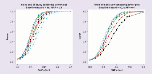
Power is estimated at a 5% significance threshold. Lines with circular points characterize the Cox proportional hazards model and lines with square points the logistic regression model. The color of the line represents the end of study time: 20 days (black); 30 days (red); 40 days (green); 50 days (blue) and 60 days (cyan).
MAF: Minor allele frequency.
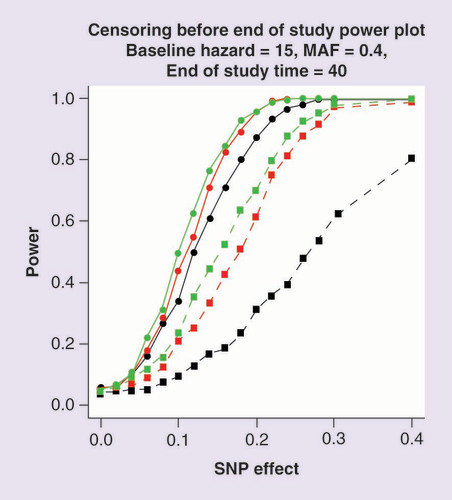
Power is estimated at a 5% significance threshold. Lines with circular points characterize the Cox proportional hazards model and lines with square points the logistic regression model. The color of the line corresponds to the rate of censoring defined by the scale parameter of the Weibull distribution: scale 20 (black); scale 40 (red) and scale 60 (green).
MAF: Minor allele frequency.
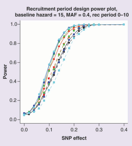
Power is estimated at a 5% significance threshold. The recruitment period is between 0 and 10 days. Lines with circular points characterize the Cox proportional hazards model and lines with square points the logistic regression model. The color of the line represents the end of study time: 20 days (black); 30 days (red); 40 days (green); 50 days (blue) and 60 days (cyan).
MAF: Minor allele frequency.
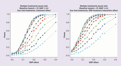
Power is estimated at a 5% significance threshold. Lines with circular points characterize the Cox proportional hazards model and lines with square points the logistic regression model. The color of the line represents the end of study time: 20 days (black); 30 days (red); 40 days (green); 50 days (blue) and 60 days (cyan).
MAF: Minor allele frequency.
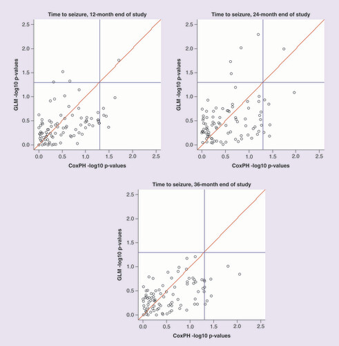
Blue lines represent 0.05 significance levels.
The Cox proportional hazards model is the basis of the most commonly applied framework for the analysis of time-to-event outcomes. It is a semiparametric model where the hazard ratio takes a parametric form in terms of the regression coefficients, but the baseline hazard is unspecified. The aim of this paper is to evaluate the power to detect association between SNPs and time-to-event outcomes under different pharmacogenomic study designs, including censoring before the end of the study, treatment effects, SNP-treatment interactions and a variable recruitment period. We will compare the power for the analysis of event times: first, under a Cox proportional hazards model and second, within a logistic regression framework with a dichotomized outcome at the end of the study. Our investigation incorporates detailed simulations and empirical evaluation in a candidate gene study of anti-epileptic drug response with SNPs mapping to/near ABCB1 [Citation5]. Although we expect that Cox proportional hazards modeling will be uniformly most powerful, our aim is to identify scenarios for which the difference in power is minimized. In these scenarios, existing GWAS analysis software for binary phenotypes could be applied to dichotomized time-to-event outcomes in an initial screen to identify SNPs for further evaluation with more rigorous, and computationally demanding, survival modeling, thereby providing insight into study design and appropriate analytical protocols.
Materials & methods
Consider a sample of unrelated patients in a pharmacogenomic study investigating the association of a time-to-event outcome with SNPs after treatment intervention. We denote the time to event for the ith patient by ti, and their treatment by a vector of covariates xi. We also denote their genotype at an SNP of interest by Si, coded under an additive dosage model (directly typed or imputed) for the minor allele. Under the assumption of proportional hazards, we can express the hazard of the event occurring at some time t in the ith individual by:Equation 1
In this model, h0(t) is the baseline hazard at time t, and the parameters βs and βx correspond to the effect on hazard of the minor allele at the SNP, and a vector of treatment effect(s), respectively.
Alternatively, we can dichotomize the time-to-event outcome of patients at the end of the study. Let yi denote the dichotomized outcome of the ith patient, given by yi = 1 if the event has occurred, and by yi = 0 if not. Note that patients who are censored before the end of the study are excluded from this analysis since we do not know whether the event has occurred or not and thus are treated as missing. Within a logistic regression framework, we can model the log-odds of the occurrence of the event by:Equation 2
In this expression, ωs corresponds to the log-odds of the minor allele at the SNP, and ωx represents a vector of treatment effect(s).
For both models, we can form a likelihood ratio test of association of the SNP with outcome by maximizing the unrestricted models (1; EquationEquation 1Equation 1 ) and (2; EquationEquation 2
Equation 2 ) and comparing with that under the null hypothesis, for which the allelic effects, βS and ωS, are zero. Both models can also be generalized to incorporate additional covariates or an SNP-treatment interaction effect.
Simulation Study
We considered four pharmacogenomic GWAS designs to evaluate SNP association with time-to-event outcomes, selected after examination of published studies in the literature, including Clarke et al. [Citation6] and Han et al. [Citation7]. The scenarios considered, described in detail below, allowed for variable end of study time and recruitment period, censoring before the end of the study, multiple treatment effects and SNP-treatment interaction. In all scenarios, we considered a study undertaken for a maximum of 60 days. However, we consider the impact on the analysis of fixing the end of the study, Z, at 20, 30, 40, 50 or 60 days. We assumed that patients who do not experience the event before the end of the study to be censored at that point. However, in some scenarios, we also allowed for the possibility of censoring before the end of the study due to the occurrence of an adverse treatment reaction or other reasons for dropout. In these scenarios, patients who are censored before the end of the study are excluded from the logistic regression analysis at the end of the study because we cannot determine whether the event has occurred or not.
For each scenario, we considered SNP effects, βs, on the hazard of the occurrence of the event in the range of 0 (null model to evaluate false-positive error rates) to 0.4. For each simulation, we generated 1000 replicates of data for a sample of 1000 patients. For each replicate, we simulated genotype data for the ith patient, Si, from a multinomial distribution with minor allele frequency of 0.4, under the assumption of Hardy–Weinberg equilibrium. The time to the occurrence of the event, ti, was simulated from an exponential distribution with scale parameter dependent on the genotype Si, SNP effect βs and other scenario-specific factors outlined below.
Scenario 1. No treatment effect & censoring occurs only at the end of the study
The hazard of the event at time t was given by
where we considered two baseline hazards: h0(t) = 15 and h0(t) = 50. A larger value for the baseline hazard means a patient's survival time is longer. Since there was no censoring before the end of the study, the observed event time for the ith patient was τi = ti if the event occurred before the end of the study; otherwise τi = Z (i.e., was replaced by the end of study time).
Scenario 2. Random censoring due to drop out before the end of the study
The hazard of the event at time t is given by
where we considered a baseline hazard of h0(t) = 15. The censoring time of the ith individual, ci, was simulated from a Weibull distribution with scale parameter 20, 40 or 60. The end of study time is fixed at 40 days, therefore a Weibull scale parameter of 20 for censoring times corresponds to approximately 50% censored observations during the study, a scale of 40 corresponds to approximately 30% censored observations and a scale of 60 corresponds to approximately 20% censored observations. If censoring occurred before the end of the study for the ith patient, they were assumed to have dropped out at that time, and their observed time τi = ci. If the simulated censoring occurred after the end of the study for the ith patient, their observed event time was τi = ti if the event occurred before the end of the study; otherwise τi = Z (i.e., was replaced by the end of study time).
Scenario 3. Recruitment period during first 10 days of the study & censoring occurs only at the end of the study
The hazard of the event is given by
where we considered a baseline hazard of h0(t) = 15. The recruitment time, ri, was simulated from a uniform distribution over the first 10 days of the study. Since there was no censoring before the end of the study, the observed event time for the ith patient was τi = ti – ri, if the event occurred before the end of the study; otherwise τi = Z - ri.
Scenario 4. Multiple treatments with variable effects on outcome & censoring
Patients were randomly assigned to one of four treatments (A, B, C or D). Treatment A increased the hazard of the event at any given time, while treatment C resulted in increased random censoring due to adverse drug reaction before the end of the study. The hazard of the event is given by
where we considered a baseline hazard of h0(t) = 15, βx = 0.2 is the effect of treatment A, and xi is an indicator variable taking the value 1 if the ith patient is assigned to treatment A, and 0 otherwise. If the patient is assigned to treatment C, censoring occurs more frequently before the end of the study, with time, ci, simulated from a Weibull distribution with a scale parameter of 10. All other treatments have a scale parameter of 30. As for Scenario 2, if censoring occurred before the end of the study, the patient was assumed to have dropped out at that time, so that τi = ci. If censoring occurred after the end of the study, the observed event time for the ith patient was τi = ti if the event occurred before the end of the study; otherwise τi = Z (i.e., was replaced by the end of study time). Under this same design, we also simulate survival times with a significant SNP-treatment interaction effect. The hazard now becomes
with βint = 0.2, and xi defined as above.
For each scenario, the event time was dichotomized at the end of the study, Z, such that the binary outcome for the ith patient, yi = 1 if ti < Z, and 0 otherwise. For Scenarios 2 and 4, patients censored before the end of the study were treated as missing for the binary outcome. For each scenario, we tested for association of the SNP with the time to event under a Cox proportional hazards model and with the binary outcome in a logistic regression framework. For Scenarios 1, 2 and 3, the linear component of the regression model included an effect of the SNP only. However, in Scenario 4, the linear predictor was extended to include an indicator variable to account for treatment (but not an interaction effect). We evaluated the power and type I error rate of each test to detect association of the SNP with outcome at a 5% significance threshold, approximated by the proportion of replicates for which p < 0.05 for the SNP effect. All simulation scripts and analyses were performed in R 3.2.0.
Application to the SANAD study
The SANAD study was initiated to investigate the impact of genetic variation on response to anti-epileptic drugs. Leschziner et al. [Citation5] considered 503 patients receiving one of six anti-epileptic drugs over a follow-up period of between 84 and 2296 days. They evaluated the evidence of association of 501 SNPs mapping to/near the ABCB1 gene with time to 12-month remission, time to first seizure and time to drug withdrawal due to inadequate seizure control or adverse reactions. Here, the original dataset was manipulated to illustrate similar designs to that of the simulation study. Specifically, we tested for association of SNPs with time to first seizure within the first 12, 24 or 36 months of follow-up using a Cox proportional hazards model. We also tested for association with a dichotomized outcome, at the same follow-up time points, in a logistic regression model. As these end of study follow-up times were implemented a censoring outcome and binary outcome were created influenced by the time-to-seizure and time-to-withdrawal outcomes. The number of missing observations due to censoring before the end of the study, for the logistic regression model at 12, 24 and 36 months, were 56, 69 and 95, of the 503 patients, respectively. Before analysis, we eliminated SNPs with minor allele frequency (MAF) less than 1% and missing genotype rate greater than 5%.
Results
Simulation study
presents the power to detect association of the SNP, under Scenario 1, with time to event using a Cox proportional hazards model and with the dichotomized outcome at the end of the study in a logistic regression framework. The two plots present power, for different end of study times, for a baseline hazard of 15 (left) and 50 (right). For a baseline hazard of 15, the majority of patients will have experienced an event by day 20, and almost all will have experienced the event by day 60. In this setting, the number of censored observations at the end of the study is low, and the Cox proportional hazards model can directly account for the times at which the events occurred. On the other hand, the logistic regression model loses power as the end of study time increases because the number of cases and controls becomes more imbalanced. As a result, the difference in power between the two models increases with the end of study time. On the other hand, for a baseline hazard of 50, far fewer events occur during the study period. As a consequence, there is less to be gained through direct modeling of event times, and the logistic regression analysis has almost identical power to the Cox proportional hazards model. An end of study of 60 is the most favorable cutoff point for the logistic regression model as it has the greatest balance of events and nonevents occurring during the trial. Supplementary Figure 1 presents a comparison of -log10 p-value and estimated effect sizes from Scenario 1 for a baseline hazard of 15, MAF of 0.4, SNP effect of 0.1 and an end of study time of 40. These parameter settings achieve a power of 50% to detect associations using the Cox proportional hazards model. These results highlight that effect sizes from the two approaches are highly correlated but the signal of association is more often stronger under the Cox proportional hazards model than logistic regression model.
presents the power to detect association of the SNP, under Scenario 2, where censoring can occur before the end of the study. As censoring increases, the power of both models decreases. However, the reduction is more dramatic for the logistic regression modeling of dichotomized outcomes because the number of patients contributing to this analysis decreases with a consequent reduction in power. Supplementary Figure 2 presents a comparison of -log10 p-value and estimated effect sizes from Scenario 2 for a baseline hazard of 15, MAF of 0.4, SNP effect of 0.1, a Weibull censoring scale parameter of 60 and an end of study time of 40. These parameter settings achieve a power of 50% to detect associations using the Cox proportional hazards model. These results highlight that effect sizes from the two approaches are again highly correlated, and the signal of association is typically weaker under logistic regression modeling of the dichotomized outcome than the Cox proportional hazards model.
presents the power to detect association of the SNP, under Scenario 3, which incorporates a variable recruitment period for patients at the start of the study. The results are similar to those observed for Scenario 1 with a baseline hazard of 15. Like Scenario 1, the difference in power between the two modeling approaches depends on the proportion of patients in which the event has occurred, and is maximized for an end of study time of 60 days because most patients will have experienced the event by this time, even with a variable recruitment period. An end of study of 20 days shows the smallest difference in power between the models because very few events occur with the majority of patients surviving to the end of the study. Supplementary Figure 3 presents a comparison of -log10 p-value and estimated effect sizes from Scenario 3 for a baseline hazard of 15, MAF of 0.4, SNP effect of 0.1 and an end of study time of 40. These parameter settings achieve a power of 50% to detect associations using the Cox proportional hazards model. As with previous scenarios, the effect size estimates obtained from the two models are highly correlated but signals of association are generally stronger under the Cox proportional hazards model than the logistic regression model.
presents the power of the two modeling approaches for Scenario 4, where time to event is dependent on treatment. The first plot (left) includes a treatment effect of 0.2 on survival times with both analysis models adjusting for the treatment covariate. The second plot (right) includes both a treatment effect of 0.2 and an SNP-treatment interaction of 0.2 but incorporates only the treatment covariate in the analysis models (because an interaction effect is not typically assumed, a priori). It is clear from both plots that as the end of study time increases, which results in more censoring during the study period, the power of the logistic regression model is substantially reduced. Introducing an SNP-treatment interaction increases power for both analytical approaches because the marginal effect of the SNP is increased, even if the interaction effect itself is not taken account of in the analysis model. Supplementary Figure 4 presents a comparison of -log10 p-value and estimated effect sizes from Scenario 4 for a baseline hazard of 15, MAF of 0.4, SNP effect of 0.1, treatment effect of 0.2, interaction effect of 0.2 and an end of study time of 40. These parameter settings achieve a power of 50% to detect associations using the Cox proportional hazards model. These results highlight that the effect sizes from the two approaches are correlated but the signal of association is more often stronger under the Cox proportional hazards model with very few replicates with more significant associations found toward the logistic regression model.
For all parameter settings, the Cox proportional hazards analysis of time to event was always at least as powerful as the logistic regression model, as expected. Across scenarios, the greatest difference in power occurred when the end of study time was extended because the number of individuals experiencing the event was maximized, and there was more information in the event times themselves. While the power of the Cox proportional hazards model stays relatively constant, that of the logistic regression approach gets substantially weaker because of the increased imbalance in the number of cases and controls.
Application to the SANAD study
depicts the -log10 p-value for association of SNPs with time-to-event outcomes from the SANAD study. Each point corresponds to an SNP, with the p-value for the SNP effect from the Cox proportional hazards model on the x-axis and the p-value for the SNP effect from the logistic regression model on the y-axis. The two blue lines indicate a nominal 5% significance threshold for association. The top left quadrant indicates significant SNPs found only by the logistic regression model, the bottom right quadrant shows significant SNPs found only by the Cox proportional hazards model, and the top right quadrant indicates significant SNPs found by both models. The key observation from this analysis is that, as the study period increases, the number of associated SNPs found by the logistic regression model is reduced. This result supports the findings of the simulation study because, as the end of study time increases, there are more censored events within the sample. For the outcomes of times to seizure at 12 and 24 months, there is little difference between significant SNPs found by the logistic regression or Cox proportional hazards models. However, for an end of study time of 36 months, the logistic regression model fails to detect any associations.
Discussion
As expected, the Cox proportional hazards model was demonstrated to be uniformly more powerful than the logistic regression analysis of dichotomized outcomes across simulation scenarios and generated stronger signals of association in the SANAD study. However, the difference in power between methods was highly dependent on the rate of censoring and number of events occurring within the study period. If few events occur and the majority of subjects survive until the end of study, then there is little to be gained by modeling time-to-event outcomes. However, the power of the logistic regression model is significantly affected by the two types of censoring: first, at the end of study because the event has yet to occur and second, during the study period because of the occurrence of an adverse event or dropout. If there is a lot of censoring during the study, these observations are treated as missing in the logistic regression model, and therefore result in a lack of power to detect associations between SNPs and outcome. The rate of censoring at the end of the study (i.e., the number of events that have occurred) will impact the ratio of cases to controls in the dichotomized outcome. For a given sample size, imbalanced studies will have less power than those for which the number of cases and controls is equal.
There are other survival models available for the analysis of time-to-event data such as Weibull regression. Parametric models, such as this, are beneficial as they assume the statistical distribution of the data and have completely specified hazard and survivor functions. We might expect the power of these approaches to be greater than the Cox proportional hazards model when the assumption of proportional hazards is not appropriate. However, we expect the scenarios in which the logistic regression model of dichotomized outcomes provides equivalent power to the survival modeling of time-to-event outcomes to hold under these alternative approaches.
The results of our study have important implications for the development of analytical protocols in the analysis of time-to-event data in pharmacogenomic studies. We have highlighted scenarios for which the difference in power between the two analysis models is minimized. In these scenarios, existing GWAS analysis software could be applied to dichotomized time-to-event outcomes in an initial screen to identify SNPs for further evaluation with more rigorous, and computationally demanding, survival modeling. Our study also highlights the need for flexible software for the analysis of time-to-event data that can efficiently handle the scale and complexity of genetic data throughout the genome.
Conclusion
The Cox proportional hazards model of time to event was demonstrated to be more powerful than the logistic regression analysis of a dichotomised outcome. The difference in power between the approaches was highly dependent on the rate of censoring. Our results highlight that initial evaluation of SNP association signals using computationally efficient software with dichotomised outcomes provide an effective screening tool for some design scenarios, and thus has important implications for the development of analytical protocols in pharmacogenomic studies.
Future perspective
The development of methodology and software for the analysis of time to event outcomes will enable implementation of efficient software that can accommodate the scale and complexity of large-scale pharmacogenetic GWAS. The advancement will offer greater power for the detection of genetic biomarkers of treatment response, enabling personalised medicine approaches for clinical outcomes in pharmacogenetics.
Background
Methodology for genome-wide pharmacogenomic studies with time-to-event outcomes is not well developed.
Materials & methods
We evaluate the power to detect associations between SNPs and time-to-event outcomes comparing two regression modeling approaches.
A wide range of trial designs for pharmacogenomic studies with time-to-event outcomes is covered.
Results
As expected, the Cox proportional hazards model is more powerful at detecting associations between SNPs and time-to-event outcomes over logistic regression analysis of dichotomized outcomes at the end of the study.
The rate of censoring and number of events occurring during the study is correlated to the performance of methods.
Conclusion
Results highlight the need for software to enable the efficient analysis of genome-wide association studies of time-to-event outcomes with a range of survival models.
Pharmacogenomic data have more complexities that need to be accounted for by the analysis, so extensions to existing methods are needed.
Disclaimer
The views and opinions expressed within this paper do not necessarily reflect those of the NHS, the HTA or the Department of Health.
Ethical conduct of research
The authors state that the SANAD study has previously obtained appropriate institutional review board approval and have followed the principles outlined in the Declaration of Helsinki for all human or animal experimental investigations. In addition, informed consent has previously been obtained from the participants involved in the SANAD study.
Supplemental Document 1
Download MS Word (106.6 KB)Acknowledgements
The authors would like to thank T Marson for allowing access to and use of the SANAD trial data.
Financial & competing interests disclosure
The original trial was funded by the HTA. The researchers are independent from the funders. SANAD is registered with the International Standard Randomized Controlled Trial Number Register and is number ISRCTN38354748. AP Morris is a Wellcome Trust Senior Fellow in Basic Biomedical Science (under award WT098017). The authors have no other relevant affiliations or financial involvement with any organization or entity with a financial interest in or financial conflict with the subject matter or materials discussed in the manuscript apart from those disclosed.
No writing assistance was utilized in the production of this manuscript.
Additional information
Funding
References
- The Wellcome Trust Case Control Consortium . Genome-wide association study of 14,000 cases of seven common diseases and 3,000 shared controls . Nature447 ( 7145 ), 661 – 678 ( 2007 ).
- Purcell S , NealeB , BrownKTet al. PLINK: a tool set for whole-genome association and population-based linkage analyses . Am. J. Hum. Genet.81 ( 3 ), 559 – 575 ( 2007 ).
- Marchini J , BandG . SNPTEST . mathgen.stats.ox.ac.uk/genetics_software/snptest/snptest.html .
- Ji Y , BiernackaJM , HebbringSet al. Pharmacogenomics of selective serotonin reuptake inhibitor treatment for major depressive disorder: genome-wide associations and functional genomics . Pharmacogenomics J.13 ( 5 ), 456 – 463 ( 2013 ).
- Leschziner G , JorgensenAL , AndrewTet al. Clinical factors and ABCB1 polymorphisms in prediction of antiepileptic drug response: a prospective cohort study . Lancet Neurol.5 ( 8 ), 668 – 676 ( 2006 ).
- Clarke T , CristRC , AngAet al. Genetic variation in OPRD1 and the response to treatment for opioid dependence with buprenorphine in European–American females . Pharmacogenomics J.303 – 308 ( 2014 ).
- Han JY , ShinES , LeeYSet al. A genome-wide association study for irinotecan-related severe toxicities in patients with advanced non-small-cell lung cancer . Pharmacogenomics J.417 – 422 ( 2013 ).