Comparative analysis of mathematical models of cell death and thermal damage processes

Abstract

The standard method for assessing hyperthermia treatment has been calculation of cumulative equivalent minutes at 43 °C, CEM₄₃ and its variations. This parameter normalises treatment thermal histories rather than predicts treatment results. Arrhenius models have been widely used in analysing higher temperature thermal treatments and successfully employed to predict irreversible thermal alterations in structural proteins. Unfortunately, in many, but not all cases they fail to represent thermally induced damage or cell death at hyperthermic temperatures, 43–50 °C, exhibiting significant over-prediction of the initial ‘shoulder’ region. The failure arises from the simplifying assumptions used to derive the irreversible reaction format that has been used in thermal damage studies. Several successful multi-parameter fit methods have been employed to model cell survival data. The two-state statistical thermodynamic model was derived from basic thermodynamic principles. The three-state model results from relaxing the assumptions under the Arrhenius formulation that result in an irreversible reaction. In other cell processes studied in vitro the irreversible Arrhenius model holds, and is sufficient to provide an accurate and useful estimate of thermal damage and cell death. It is essential in numerical model work to include multiple thermal damage processes operating in parallel to obtain a clear image of the likely outcome in tissues. Arrhenius and other C(t) models have that capability, while a single value for CEM₄₃, does not.

• Modelling
• targets of cellular thermal damage
• thermal dosimetry

Introduction

The concept of thermal dose units, in the form of cumulative equivalent minutes (CEM) of exposure at 43 °C, dates at least from the pioneering work of Sapareto et al. in 1977 [1] and 1978 [2] and is well described in their chapter in the subsequent 1982 book [3]. The Arrhenius formulation description of thermal damage processes was first employed by Henriques and Moritz in 1947 to describe the genesis and development of thermal contact skin burns in pigs [4–7]. Additional studies by Fugitt [8] and Weaver and Stoll [9] and many others confirm the applicability of these models to that process. The underlying physical principles of the two descriptions are the same; however, their application and significance are quite different.

Thermal dose units (i.e. CEM) constitute a normalising method for thermal histories: a particular thermal exposure is scaled into an equivalent exposure time at the reference temperature, typically 43 °C. The Arrhenius formulation, in the form of absolute reaction rates, is designed to predict the ‘yield’ of a reaction, i.e. the fraction of product formed, or fraction of remaining reactants – although the original 1947 skin burn analyses and subsequent applications of the method by other authors did not extend to a damage fraction prediction. In thermal damage analyses reaction yield calculations can be used to estimate the volume fraction of damaged tissue constituent, or the probability of observing a particular discrete damage event in an ensemble of experiments [10–13]. Thermal dose units (CEM) effectively normalise different thermal histories but do not, per se, provide a prediction of outcome in the tissues of interest.

The typical assessment criterion in hyperthermia work is to regard a CEM value in excess of a defined threshold number of minutes, for example, 60 min, as evidence of an effective treatment, or an estimate of a treatment physical boundary. He et al. [14] and others, e.g. Nadall et al. [15], point out that above about 50 °C CEM values do not correlate with the observed thermal alterations. The He et al. 2009 paper [14] presents some standards of comparison and a method of conversion between Arrhenius and CEM parameter calculations.

It is tempting to apply Arrhenius predictions to so-called ‘cell survival’ curves, and to apply the original definition of CEM to derive an estimate of an Arrhenius prediction, since inspection of the respective physical bases reveals that there is a simple exponential relationship between them, as has been described [14]. However, in many (but not all) cases Arrhenius predictions of cell survival curves at moderate hyperthermic range temperatures (43–48 °C) grossly over-predict the thermal damage fractions in the early stages of heating, during the early stage ‘shoulder’ region, as will be shown. Many experimental measurements of dye uptake in vital stain studies and loss of clonogenicity characteristically show a slowly developing shoulder, where the rate of decrease in measured signal, C(t), increases until a relatively constant region (in a logarithmic sense) is reached.

It should be noted here that, while usually called ‘cell survival’ curves in the literature, the particular damage process measured was actually the loss of clonogenicity, whether the cells survived or not. The underlying reasons for the failure of simple irreversible Arrhenius predictions in these cases are clearly revealed by several approaches that have been presented. Among them are a probabilistic exercise in curve fitting with two parameters by Mackey and Roti Roti in 1992 [16], a ‘three compartment’ reaction-based model by O’Neill et al. [17], a ‘two-state’ model derived from statistical thermodynamic considerations by Feng et al. [18], and an elegant biochemical model by Eissing et al. [19] that describes the caspase cascade, a hallmark of the apoptosis intrinsic cell death process.

This study: (1) briefly reviews the foundations of the two commonly used methods, Arrhenius and CEM, (2) describes the underlying protein biochemistry of the caspase cascade, which is characteristic of apoptosis, (3) compares the Arrhenius method of prediction to the more accurate multi-parameter and two-state models, and (4) illustrates the utility of including multiple parallel thermal damage processes in numerical model work to provide a clear picture of the expected results in an example laser heating case. The physical bases of the various models are explored for similarities and implications. Finally, an improved approach to cell survival curve modelling is suggested.

Foundations of thermal dose units: relative reaction rates

Thermal dose units derive from the original cell survival measurements of Sapareto et al. [2] in CHO cells. The remaining clonogenically active fraction at constant temperature is calculated, in which the temperature-dependent slope of the constant-rate region in the survival curve, D₀, is the time constant of cellular response in this definition: where there are N₀ viable cells at time t₀, S = the remaining number of colony-producing cells at time t (min) at constant temperature, T, and D₀ = the time constant (min). The slope, D₀, is measured during the relatively later-developing constant-rate region of the survival curve. That is, after the shoulder region in the early stages of a typical survival curve plot of log{S/N₀} vs t – where the slope dS/dt changes rapidly – a constant rate, D₀, is observed. In these later stages of heating, the time for the population to decrease by a factor of e is constant, D₀ [20].

The original measurements [20] show a breakpoint in the Arrhenius plot at 43 °C, and that value was chosen as the reference temperature. A breakpoint in an Arrhenius plot indicates that different thermal processes dominate the observations on either side. Sapareto et al. [20], Lepock and Kruuv [21] and others describe this particular breakpoint as an indication of the upper limit at which thermo-tolerance can be induced in the cells (by the action of heat shock proteins, shepherd proteins which assist malformed proteins in regaining their original conformation), rather than an indication of two different modes of cell death. The definition of ‘viability’ is a somewhat delicate matter [22]. While loss of clonogenicity does not necessarily imply cell death – certainly, fully differentiated cells such as muscle or nerve are alive but not reproducing – if cancer cells remain alive but have lost their ability to proliferate, one of the six hallmarks of cancer, a successful result may be claimed.

Based on these observations, and on subsequent observations by other authors in different cell lines [23–25], a normalised time of exposure was suggested to provide a means for quantising hyperthermia treatments, CEM, or cumulative equivalent minutes at 43 °C. The applied thermal dose, CEM, is calculated from: where the exposure is either in discrete intervals, t_i, or continuous, and R_CEM is the ratio of exposure times required to result in the same survival for a 1 °C rise in temperature. The typically used R_CEM = 0.5 for temperatures above 43 °C and 0.25 for temperatures below the breakpoint dates from the Chinese hamster ovary (CHO) cell experiments: that is, the rate of cell death approximately doubles for every 1° rise in temperature above 43 °C. In practice, since the CEM method provides only a single number, clinical assessment methods usually calculate an effective relative volume of adequately treated tumour tissues, as developed and recently reviewed by Dewhirst et al. [26].

The thermal dose unit formulation is derived from experiment, but has its origins in the experimental work of Svanté Arrhenius in 1889 [27]. Prior to Arrhenius’s observations, strictly thermodynamic approaches assumed equilibrium conditions pertained during chemical transformation processes. Kinetic analysis, as he introduced, describes the rate at which thermal processes occur, a non-equilibrium description. The original German language publication is well explained by Johnson, Eyring and Stover in their 1974 book [28]. Briefly, Arrhenius’s experiments on reaction velocity showed a temperature dependence that could not be explained by the relative thermal energies of the reactants. The relative reaction velocities were fitted by: where k = the reaction velocity (s⁻¹) at absolute temperatures T₁ and T₂ (K), and μ is the fit parameter (dimensionless) as originally used by Arrhenius [29]. The fit parameter (Table I) was subsequently determined to be: μ = 2 E_a/R, where E_a (J mol⁻¹) is the ‘activation energy’, and R = 8.3143 (J mol⁻¹K⁻¹) is the universal gas constant [28]. The concept of an activation energy barrier and a transition state between reactants and products, E_a, was introduced by Henry Eyring to provide a physical basis for the reaction kinetics [28]. Equation (3) constitutes the theory of relative reaction rates. Several of the experimentally determined values for μ are listed in Table I [29].

Table I. Selected kinetic coefficients, μ, for relative reaction rates, Equation (3) [29].

	Fit coefficient	Ea
Process	μ	(kJ mol^−1)
Spontaneous destruction
Dibromosuccinic acid	22 200	92.3
Compound haemolysin	198 500	825.2
Rennet, 2%	90 000	374
Pepsin, 2%	75 600	314
Trypsin, 2%	62 000	258
Emulsin, 0.5%	45 000	187
Invertase, from yeast	72 000	299
Digestion
Casein by trypsin	37 500	156
Powdered casein by trypsin	7400	30.8
Egg white by pepsin	15 570	64.7
Emulsion of egg yolk by  pancreatic juice	13 600	56.5
Coagulation, precipitation
Egg white by heat	135 600	564
Egg white by sulphuric acid	11 000	45.7
Haemoglobin by heat	60 100	250
Haemolysis by heat	64 000	266
Haemolysis in the presence of  acids, bases and lysins	25 000 to 30 000	104 to 125
Milk by rennet	20 650	85.8
Killing
Bacillus typhosus	92 000	382
Bacillus paratyphosus in phenol	48 600	202

Recasting Equation (3) in terms of the relative reaction times, rather than velocities, reveals the time scaling ratio used in hyperthermia studies, R_CEM: and the classical physical chemical basis for Equation (2) is now readily apparent, where T₁ is the reference temperature.

R_CEM depends much more strongly on the activation energy, E_a, than it does on the temperature; representative values are given in Table II, computed at T₁ = 317.16 K =44 °C. At 43 °C R_CEM = exp(−1.199 × 10⁻⁶ E_a), while at 50 °C R_CEM = exp(−1.148 × 10⁻⁶ E_a), so it is not a constant, actually, and is temperature sensitive according to Equation (4). For uniform computation of CEM values the representative value for R_CEM has historically been taken to be 0.5 above 43 °C (0.428 for human tissues in vitro with a breakpoint at 43.5 °C) and 0.25 below 43 °C (0.233 for human tissues in vitro) [26,30]. By default, damage processes are usually referred to the 43 °C reference point.

Table II. Collected representative Arrhenius kinetic coefficients for heating processes.

	Arrhenius process parameters
Process	A (s^−1)	Ea (J mol^−1)	RCEM 44 C	Notes
Cell death
Sapareto [20]	9.386 × 10^101	6.344 × 10^5	0.467	Asynch. CHO cells, T > 43 °C
Beckham [80]	6.9 × 10^116	7.3 × 10^5	0.417	Without Hsp70 production
	3.7 × 10^157	9.8 × 10^5	0.309	With Hsp70 production
He [14]	2.53 × 10^24	1.684 × 10^5	0.818	Hu. BPH; EthD-1
	1.79 × 10^23	1.613 × 10^5	0.825	BPH; apoptosis and necrosis
Bhowmick [72]	1.66 × 10^91	5.68 × 10^5	0.506	AT-1 cells <50 °C, 3 h culture
	173.5	1.97 × 10^4	0.977	AT-1 cells >50 °C, 3 h culture
Borrelli [81]	2.984 × 10^80	5.064 × 10^5	0.545	BHK cells
He [62]	4.362 × 10^43	2.875 × 10^5	0.708	SN12 cells, suspended
	3.153 × 10^47	3.149 × 10^5	0.685	SN12 cells, attached
Arrhenius [29]	**2.02 × 10^60	3.82 × 10^5	0.635	B. typhosus
Arrhenius [29]	**9.40 × 10^29	2.02 × 10^5	0.786	B. paratyphosus in phenol
Shah [82]	3.495 × 10^31	2.295 × 10^5		HepG2 cells, suspended
Shah [82]	5.396 × 10^36	2.486 × 10^5		HepG2 cells, attached
Erythrocytes
Lepock [83]	7.6 × 10^66	4.55 × 10^5	0.579	Haemolysis
Arrhenius [29]	**5.72 × 10^40	2.66 × 10^5	0.729	Haemolysis
Przybylska [84]	*1.08 × 10^44	2.908 × 10^5	0.705	Haemol. normal
	*3.7 × 10^43	2.88 × 10^5	0.708	Down’s syndrome
Skin burns
Henriques [4]	3.1 × 10^98	6.28 × 10^5		NOT recommended
Diller [11]	8.82 × 10^94	6.03 × 10^5	0.485	T ≤ 53 °C (same data)
	1.297 × 10^31	2.04 × 10^5		T > 53 °C
Weaver [9]	2.19 × 10^124	7.82 × 10^5	0.391	T ≤ 50 °C
	1.82 × 10^51	3.27 × 10^5		T > 50 °C
Brown [66]	1.98 × 10^106	6.67 × 10^5	0.449	Microvascular disruption
Collagen
Pearce [41]	1.61 × 10^45	3.06 × 10^5		Birefringence loss, rat skin

*The value for A has been estimated from Wright’s line, Equation (17a).

**The value for A has been estimated from the He-Bischof line, Equation (17b).

Asynch: Asynchronous; Hu: Human; BPH: Benign Prostatic Hyperplasia; Haemol: Haemolysis.

Arrhenius formulation: absolute reaction rates and transition state descriptions

A more complete review of the thermodynamic/kinetic basis for Arrhenius thermal damage predictions may be found in several recent publications [11–13,31]. Briefly, in a bi-molecular reaction, reactants A and B surmount an activation barrier to form an activated complex in the transition state, AB*, which either relaxes back to the native state or progresses to form products according to the Gibbs free energy of formation for the activation process, ΔG* = ΔH* − T ΔS* [32–34]. The resulting reaction velocity, k, is described by the Eyring-Polyani equation: [35,36] where ΔH* = the activation enthalpy (J mol⁻¹), ΔS* = the activation entropy (J mol⁻¹K⁻¹), T = temperature (K), R = the gas constant (8.3143 J mol⁻¹K⁻¹), N = Avogadro’s number (6.23 × 10²³mol⁻¹), h_P = Planck’s constant (6.63 × 10⁻³⁴ J s), and E_a = the activation energy (J mol⁻¹). In practice ΔS*/R >> 1 and E_a = ΔH* − RT  ΔH* for first order reactions. The method is equally useful to describe uni-molecular denaturation of native state molecules, where the activation process forms an activated complex, CC* that, after some delay [37], can either relax back to undamaged or progress to damaged tissue constituents, again at overall velocity, k. where k_a = the velocity of activation, k_b = the velocity at which the activated complex relaxes back to the native state, and k_c = the velocity at which activated complex denatures to state D. The ‘steady state principle’ asserts that the rate of formation of the intermediates is equal to the rate of disappearance, so that:

Of course, C* is neither measurable nor calculable. Two limiting cases result: 1) k_b[C] > k_c, and k  (k_c k_a/k_b) and the process is first order, or 2) k_c >> k_b[C] and the process is second order. The first case applies in liquid phase systems as long as [C] is appreciable and results in an irreversible reaction with overall velocity k determined from two constant parameters, as in Equation (5). This relation will prove instrumental in understanding the discussion of the three-state model for metabolic cell death presented by O’Neill et al. to be discussed in a later section of the paper [17].

The remaining first-order reactant (i.e. the undamaged tissue constituent), C(τ), is found from the solution of the single governing Bernoulli differential state equation for an irreversible reaction: where C(0) is the original concentration of tissue constituent. The original damage parameter, as used by Henriques and Moritz, Ω(τ) [4,7], is related to the kinetic formulation by: where A = the ‘frequency factor’ (s⁻¹) and E_a = the activation energy (J mol⁻¹) are the Arrhenius coefficients for the damage process, and must be determined experimentally. Equations (5), (8) and (9) constitute the theory of absolute reaction rates, as described by Eyring, and are based on the assumption of a single transition state energy barrier with an irreversible molecular flux [35,36,38].

Comparison to the relation for reaction velocity in Equation (5) suggests that A should be treated as temperature dependent; however, the temperature in Kelvin varies so little over the range of a typical experiment or thermal treatment, especially when compared to the hyperbolically exponential dependence on temperature in the enthalpy term, as a practical matter it is not important to include the linear dependence of A on temperature. We can quickly see that for two thermal histories, T₂ = T₁ + 1, with the same resulting damage, and Ω₂ = Ω₁, the result presented by He et al. [14] follows directly from Equation (9) – because T₂ − T₁ = 1 (K):

In their original skin burn work, Henriques and Mortiz calculated only Ω values, and defined Ω = 0.53 to correspond to superficial irreversible erythema (first-degree), Ω = 1.0 to trans-epidermal necrosis (partial thickness, or second-degree), and Ω = 10⁴ to complete involvement of the dermis (full-thickness, or third-degree). It should be noted that their reported Ω values refer to the thermal history at the skin surface – i.e. to the temperature of water flowing through a metal block applied to the skin surface. A word of caution is in order: the Arrhenius values for A and E_a reported by Henriques and Moritz have since been widely used, but do not fit the original data very well. Diller and Klutke [39] re-analysed the original data and the values listed in Table II are recommended instead. See also Diller et al. and Pearce [11, 31]. Incidentally, there is a breakpoint in the original data at 52 °C above which the activation energy decreases by a factor of about 3. Likewise, Weaver and Stoll found a breakpoint at 50 °C in their studies [9].

Proper interpretation of thermal damage predictions

Looking at Ω alone masks the actual thermal events, and often leads to incorrect interpretations of predictive work as a result. It is not unusual to see either Ω = 1 or Ω = 0.53 referred to as the ‘threshold’ of thermal injury, based on the original studies. Inspection of Equation (9) shows that at Ω = 0.53 the transformation process is 41.1% complete (58.9% survival), and at Ω = 1 it is 63.2% complete – well on the way to complete damage – and consequently does not really constitute a threshold at all. Ω = 0.1 – i.e. C(t) = 90.5% or about 10% damage – is a more appropriate criterion for the threshold of thermal damage – e.g. the point at which damaged tissue constituents would likely be reliably detectable amid biological variation in a histological cross-section. In general terms ‘threshold’ means the first reliably observable change, not the ‘sure kill’ criterion, for which 90% (i.e. C(t) = 10%) is more appropriate. Large values for Ω, as are often encountered in literature, have no useful physical significance: when Ω exceeds 10 – i.e. C(t) = e^−Ω=<5 × 10⁻⁵ – the damage process is fully developed, so no new information is added by continuing to accumulate the Ω integral.

Formulation of a damage prediction in terms of remaining undamaged tissue constituent, C(τ), as in Equation (9), has substantial advantages over leaving the prediction in terms of Ω alone: 1) it directly reveals what is happening in the tissues, and 2) the prediction of C(τ) can be directly compared between numerical model results and histological analyses or functional imaging based on a quantitative measure. This method has been used successfully for several decades to predict and analyse multiple irreversible thermal alterations in structural proteins, such as collagen, actin, myosin and elastin [40–47].

Limitations of the Arrhenius integral method: particular attention to clonogenicity loss prediction

There are several important limitations to keep in mind when using the absolute reaction rate method of prediction. First and perhaps foremost, it is not functionally capable of representing the ‘shoulder’ region of experimental survival curves for many cell processes, as shown in Figure 1 for the CHO cells at 43 °C. Clonogenicity and survival curves plotted as log{S/N₀} versus linear time, as in Figure 1, often have a slowly developing ‘shoulder’ region during which the slope, 1/D₀(T) is increasing. After some time the slope approaches a constant value, the ‘constant rate’, in which region the single constant value for D₀(T) is determined, see, for example, the CHO curves [3,20]. Since the calculation in Figure 1 was performed at 43 °C the horizontal axis is also CEM. The over-estimation of cell death (actually loss of clonogenicity in these experiments) in the shoulder region is characteristic of Arrhenius-based predictions in many, but not all cell processes. This failure to represent the curve shape means that the Arrhenius model lacks sufficient physical basis to describe these cellular responses. We note that the constant slope in the Arrhenius prediction in Figure 1 is parallel to the experimental data after about 60 min, the end of the shoulder region.

Figure 1. Loss of clonogenicity curve for asynchronous Chinese hamster ovary (CHO) cells (triangles) compared to an Arrhenius prediction (solid line) with A = 2.84 × 10⁹⁹ (s⁻¹), and E_a = 6.18 × 10⁵ (J mol⁻¹), (Table II) as derived from the constant rate regions of the original data [20]. The shoulder region lasts for the first 60 min in this measurement. The Arrhenius prediction (straight line) substantially overestimates the cell death rate. A 50% loss of clonogenicity occurs at about 32 min in the experimental data, asynchronous cells are shown. An additional probabilistic model, presented by Mackey and Roti Roti [16] is also shown (to be discussed in a later section). The probabilistic model separates G1-phase (—) and S-phase (— - —) CHO cells.

Second, the absolute reaction rate calculation of Equation (9) models only a single irreversible reaction. Cell death processes often involve intricate multi-constituent functional protein cascades (as opposed to the much simpler structural proteins) with multiple interacting feedback pathways, and the irreversible single reaction formulation is inadequate to describe the observed events. So it is of little wonder that the formulation of Equation (9) does not constitute an adequate description of the events associated with cell death in many cell processes at the moderate temperatures typical of hyperthermia treatments.

Third, the relation of Equation (9) will predict damage accumulation at low temperatures for very long durations even at temperatures that are known to be below thermal damage thresholds. In fact, the model of Equation (9) is not valid below the lowest temperature at which the particular damage process has been observed. This is one advantage of the relative reaction rate formulation: an initiation temperature is specified when the reference temperature is set, and thermal damage is generally not accumulated below this value. The probabilistic model of Mackey and Roti Roti [16], as shown in Figure 1, provides separate predictions for cells in G1 and S phase in the cell cycle and is discussed in a following section. This model displays easily identifiable shoulder regions and the two predictions straddle the experimental measurements in the asynchronous cell population.

Application to thermal damage, loss of clonogenicity and cell death predictions

Arrhenius models have proven very effective in processes that more likely involve only single irreversible reactions, such as denaturation of structural proteins. Oftentimes, cell death processes involve the extremely intricate cascades of functional proteins that typify the intrinsic cell death mechanisms. The complex multi-component nature of these processes explains why Arrhenius predictions fail in many cases, and warrants some discussion at this point.

Brief description of intrinsic cell death processes

Thermally induced intrinsic cell death processes – programmed cell death (PCD) – over the moderate temperature ranges and longer heating times typical of hyperthermia treatments involve intricate cascades of functional protein signalling and effector systems composed of numerous feedback pathways and cooperating reactions. The Arrhenius formulation, including CEM calculations, describes an irreversible single first-order reaction with two constant parameters, more typical of structural proteins, and is thus somewhat ‘reductionist’, as it were, in comparison. The functional aspects of structural proteins are essentially determined entirely by their chemical formulation and simpler periodic geometry; while for functional proteins the conformation (i.e. folding) and morphology are at least equally important, and usually dominate. In fact, ‘activation’ of a functional protein may simply involve a slight shape change to reveal a catalytic site [48]. Intrinsic cell death processes are orders of magnitude more complex than single first-order irreversible reactions.

Intrinsic cell death processes

Four intrinsic cell death processes are currently under intense study. The most prominent among them is apoptosis, which represents the vast majority of the literature – most of it within the last 15 years – because of its implications for disease states from HIV-AIDS and auto-immune diseases to cancer. Recently, necroptosis has been differentiated from the apoptosis mechanism in that it follows caspase-independent pathways, while the caspase cascade is a cardinal feature of apoptosis [49–51]. Caspases are cysteine aspartic proteases that cleave and disassemble multiple functional and structural proteins – notably the cytoskeleton and related molecules that comprise the cell scaffold. Necroptosis (intrinsic), like necrosis (extrinsic), releases cytosolic fragments into the extracellular space, while the end-stage action of caspases in apoptosis is to disassemble the cytoskeleton and bleb the plasma membrane and cytosolic fragments into completely enclosed apoptotic bodies. The apoptotic bodies contain the cytosolic components and, due to activation of the normally inactive scramblease on the cytosolic leaflet of the plasma membrane, the non-cytosolic surface presents signal proteins that attract macrophage engulfment [48,52].

Autophagy is the intrinsic mechanism that surrounds and sequesters severely badly behaved proteins and foreign bodies into endosomes that often eventually incorporate low-pH lysosomes. Sequestered proteins can be disassembled into basic subunits for eventual re-use (a recycling survival mechanism), or a decision can be made to kill the cell in severe cases. An excellent recent review of autophagy may be found in the recent paper by Zhang and Calderwood [53]. Finally, pyroptosis is cell death resulting from caspase-1 activation by a pyrogen, such as interleukin (IL-1 or IL-6), if the insult is sufficiently strong [54]. The complex nature of these processes can be more fully appreciated by inspecting what is presently known about apoptosis, the best understood among them at this point.

Biochemical model of apoptosis: the caspase mechanisms

Apoptosis has many intrinsic and extrinsic trigger mechanisms. An example intrinsic signal mechanism is the p53 pathway, in which the ‘guardian of the genome’, nuclear protein p53, detects stress-induced malformed DNA, and initiates the release of cytochrome c from the inter-membrane spaces of mitochondria. Cytochrome c, Apaf-1 and caspase-9 form an apoptosome (a so-called ‘wheel of death’) that cleaves and activates many molecules of executioner caspases (C3, C6 and C7), which in turn cleave and activate others in a chain reaction that builds to cell death. Cytochrome c also has a vital role in oxidative phosphorylation in the mitochondria, where it acts as an electron transporter between complexes III and IV in the electron transfer chain during the final stages of ATP production [55]. There are many other intrinsic signal pathways of similar complexity. An example of an extrinsic pathway is the activation of a plasma membrane death receptor ligand by a tumour necrosis factor (Tnf) family protein – TRAIL are ‘TNF-related apoptosis-inducing ligands’ – such as Fas, which causes the release of ‘death inducing signalling complex’ (DISC), e.g. ‘Fas-associated death domain’ (FADD), which then recruits procaspase-8 (or C10), in turn activated by autocatalytic cleavage [48,52].

A landmark paper by Eissing et al. [19] presents a substantially simplified model of apoptosis that clearly illustrates the inherent complexity of the caspase mechanisms. Their simplified biochemical model treats the caspase block alone, as shown in Figure 2. In their model all of the initiator caspases (C2, C8, C9, C10) are represented by caspase-8, while all of the executioner caspases (C3, C6, C7) are represented by caspase-3.

Figure 2. Simplified caspase feedback control block as used in the numerical models of apoptosis [19] tBid is truncated (cleaved) Bid, which enters the mitochondrial inter-membrane space and releases cytochrome c and Smac/DIABLO. The many inhibiting inputs (i.e. BAR) have been eliminated for clarity. Other unused proteins are also sent for degradation (not shown in this figure).

The IAP in the figure are ‘inhibitor of apoptosis proteins’ [56] – for example, some members of the Bcl-2 family – which bind activated C3 (i.e. C3*) for a variable time that depends on the strength of the input signal, activated caspase-8, C8*. This delay action essentially determines the time for apoptosis to appear after the input signal is received.

The biochemical model includes four overall law of mass action reactions:

As is typical in biochemical systems, the overall reactions consist of many intermediate steps. The four overall reactions are governed by eight dynamic state-space equations:

In these state equations the tilde (∼) indicates binding, and the BAR are ‘bi-functional apoptosis regulator’ proteins, for example other members of the Bcl-2 family, which consists of both pro- and anti-apoptosis proteins. The ‘i’ prefix indicates temporary inactivation by binding. The various ‘k’ are reaction velocities, each of which can reasonably be expected to individually follow Arrhenius kinetics. Equations (12) constitute a quasi-linear systems model, a familiar construct in transient electric circuits, control systems and signal processing analyses. We also note that each of the reactions has both forward (−k[C]) and reverse (+k[C]) components. Eight governing state space equations mean that the dynamic response can be anywhere between first- and eighth-order, depending critically on the particular feedback mechanisms.

Their model results show that the single cell response dynamics are very sensitive to the strength of the input signal. Figure 3 has output (C3*) delays between 200 and 2000 min (3.3 and 33 h) depending on the input signal level (3000 to 750 molecules/cell, respectively). The output response signal appears to be from either an approximately critically damped or slightly under-damped second-order or, perhaps, a third-order characteristic equation.

Figure 3. Model calculations of the dynamic response of the C3* output to input signal strengths (C8*) at 750 and 3000 molecules/cell [19]. Copasi 4.8 was used to make the calculations based on a model file kindly provided by Thomas Eissing.

In additional models, the authors applied stochastic analysis to model a population of cells. The input signal probability density function (pdf) is illustrated in Figure 4B, and the resulting dynamic response of the cell population in Figure 4A. Note that the delay between initiation and appearance of substantial amounts of C3* output signal in the population is dominated by the peak in the input signal strength in the pdf, as would be expected. These results are held by the authors to explain the differing kinetics between those of a single cell and of a population of cells. The probabilistic aspect of this analysis provides some insight into the advantage of including a stochastic process in curve fitting, as was done by Mackey and Roti Roti [16]. Their probabilistic model is discussed in the next section.

Figure 4. (A) Plot of the stochastic response of a population of cells. (B) Plot of the probability density function (pdf) impressed on the strength of the input signal, C8*, that resulted in part (A) response [19].

Plainly, however instructive they may be, detailed biochemical models are far too cumbersome to be practical in modelling either cell survival curves or hyperthermia treatments. Several approximate model constructs have been suggested to provide reasonable predictions of cell survival curves and other cell death processes that are functionally sophisticated enough to provide accurate predictions.

Models of cell survival and loss of clonogenicity curves

The failure of Arrhenius analyses to accurately represent early stage loss of clonogenicity and other processes in many cell types should not be surprising in view of the complexity of the system of functional protein cascades that are likely to be involved. The degree of over-estimation typical of the early stage shoulder region was seen in Figure 1. The poor fit is most likely attributable to: (1) Arrhenius analysis as currently used describes a single first-order irreversible reaction with two constant parameters and does not include some sort of delay feature, (2) the coefficients are determined from the constant-rate portion of the survival curve, after a relatively long time has elapsed, and (3) the functional form is not mathematically adequate to represent the experimentally observed curve shape, specifically the shoulder region. A number of two- and three-parameter fits to cell survival curves have been proposed in recent decades, and were reviewed by Wright in 2011 [57]. Representative processes are studied in some detail in this section.

Stochastic model of clonogenicity loss

In 1992 Mackey and Roti Roti developed a probabilistic model of the loss of clonogenicity from their own CHO cell line experiments [16]. Their model was somewhat heuristically postulated, derived from curve fitting and assumes a normally distributed cell population described by a temperature-dependent parameter, ε(T, t), which represents the relative clonogenicity of a single cell. A value of ε below ε_min = −3 indicates that a cell has lost clonogenicity in their model. Initially the mean value of a cell population, ε_m, is set to zero with standard deviation = 1, and a Gaussian probability density function is impressed on the population (see Figure 5):

Figure 5. Sketch of the shift of a population of G1 phase CHO cells in the probabilistic model of Mackey and Roti Roti as temperature increases from an initial 37 (ε_m = 0) to ε_m = −5 at 43 °C after a long time [16].

As heating progresses, the mean value for the population decreases according to an Arrhenius-like term with a time delay that reflects the relative speed of the response to a step change in temperature. Heating at constant temperature establishes a new steady-state mean value, ε_F, according to:

In this representation hypothetical equivalent Arrhenius parameters have been impressed on the function that were not part of the original publication to help reveal the kinetic behaviour. The population mean, ε_m(t), then responds to a temperature change according to the step response, s(t):

CHO cells in G1-phase are less heat sensitive than cells in S-phase in their work [16]. Correspondingly, for the G1 cells the fit coefficients are: a₀ = 201 (corresponding to A = 1.96 × 10⁸⁷), a₁ = −6.3 × 10⁴ (corresponding to E_a =5.24 × 10⁵J mol^-1), and k = 1.54 × 10⁻⁴ (s⁻¹). For the S-phase CHO cells: a₀ = 211 (this value corrects a typographical error in the original publication, and corresponds to A = 4.33 × 10⁹¹), a₁ = −6.59 × 10⁴ (E_a = 5.48 × 10⁵J mol⁻¹), and k = 4.0 × 10⁻⁴ (s⁻¹), almost three times faster than the G1-phase cells. At a temperature of 43 °C ε_F = −5.66 for the G1-phase cells and − 12.95 for the S-phase cells. Prediction of the survival curve shape is dominated by the response speed and the normal distribution probability density function. For comparison, 50% loss of clonogenicity at 43 °C occurs at τ = 82 min for the G1-phase cells using this model, and at 13 min for the S-phase cells – compared to 32 min for the asynchronous CHO cells in the experimental data plotted in Figure 1.

At any time the surviving cell fraction is calculated from the density function by:

Implementation of the probabilistic model in a numerical calculation with transient temperatures requires the impulse response, h(t), associated with the step response, s(t), of Equation (15):

During transient model execution the applicable exp{−kt} term can be ‘deconvolved’, as it were, from the current value of the population mean by Equation (15).

Three compartment three-parameter model of cell survival curves

Recently, O’Neill et al. suggested a three-compartment model for cell survival curves that relies on three parameters to obtain a good fit [17]. The form of the overall governing ‘reaction’ is actually identical to Equation (6). where A = the alive cell fraction (i.e. not the Arrhenius fit parameter), V = a fraction of vulnerable cells that may recover to state A, and D = the dead cell fraction. The sum of the three states is always 1, so the dynamic system state-space equations reduce to: where state V has been eliminated by enforcing continuity to reduce the number of variables. We note that the first term on the right hand side of Equation (19a), the forward flux, is identical to Equation (8). We also note that enforcing the net forward rate and ‘activation’ rate, as it were, to be equal – both are k_f – seems to challenge continuity constraints; certainly it violates the steady-state principle upon which Equations (7) were derived. The authors’ rationale that: ‘there is a single damage process that incorporates all physiological damage mechanisms’ and that ‘the vulnerable state is an arbitrarily set position along the fast path’ does not fully address this issue. However, that is the construct under which the model parameters were derived from the experimental curves and may be acceptable if the backward rate, k_b, is very small compared to k_f – their results do not support this case, so it may be something of a matter for further consideration. The overall framework in this model essentially relaxes the primary assumptions regarding the relationships among k_a, k_b, and k_c under Equation (7) that were enforced to obtain Equation (8). The fit that they obtained is far superior to the simple analysis of Equation (8) for the metabolic process they studied.

Two cell lines were heated at constant temperatures, HepG2 (human hepatocarcinoma) and MRC-5 (human lung fibroblasts), and subsequently cultured for varying periods at 37 °C. The cell death measure was loss of fluorescence at 490 (green) and 650 nm (red) wavelengths, indicating reduced metabolic processes according to the authors. In a separate communication, it was determined that the vital stains used were fluorescein diacetate and propidium iodide (PI) [58]. The experimental data for the two separate cell lines and combinations of them were fitted by: where k_f0 (s⁻¹) and T_k (°C, surprisingly), are fit parameters, along with k_b (s⁻¹), and T is also in (°C); it is a bit surprising to find Celsius degrees used in the fit. If the initial value of A (i.e. alive cells) is set to 1.0 a trivial solution results (and the process never begins), so the initial value is set to A₀ = 0.99 in their model, forcing V₀ = 0.01.

For cells cultured for after 2 h after heating, the HepG2 cells alone have: k_f0 = 0.80 × 10⁻³ (s⁻¹), k_b = 0.25 × 10⁻³ (s⁻¹) and T_k = 24.6 (°C). For the MRC-5 cells alone: k_f0 =9.07 × 10⁻³ (s⁻¹), k_b = 19.2 × 10⁻³ (s⁻¹) and T_k = 63.5 (°C). The MRC-5 cells are more thermally robust than the HepG2 cells, and both cell lines appear to be quite thermally robust in this process assay since some viability is maintained for 2 h after 5 min of exposure to 100 °C. The paper has fit coefficients for mixtures of these cells, and also a ‘slow death’ model for cells during long-term incubation at 37 °C after the heating regimens conclude. Briefly, if less than 70% of the cells remain viable 2 h post-heating, all of them in the group will die during the next several days. In subsequent publications the research group have stated that the mode of cell death in the hyperthermia experiments was apoptosis [59–61].

O’Neill et al. [17] report Arrhenius fit parameters of A = 769 (s⁻¹) and E_a = 3.7886 × 10⁴ (J kg⁻¹). The basis for these calculated values is not completely specified, and the units are not what one ordinarily expects to see in this sort of analysis. Regression analysis of the reported combined cell viability data at 2 h post-heating in units used in this paper yields an Arrhenius fit of A = 2.71 × 10¹⁵ (s⁻¹) and E_a = 1.323 × 10⁵ (J mol⁻¹) with some significant scatter in the data: r²= 0.516. These recalculated coefficients do not fit their experimental data any better than the ones they have used in comparison calculations in the paper.

Two-transition-state model of cell survival curves

Feng et al. [18] present an alternative method derived from a two-transition-state statistical thermodynamic analysis. This model has the advantage over some of the other multi-parameter fits that it was derived directly from thermodynamic principles, and is interesting for that reason. The results presented by Eissing et al. [19] suggest that multi-state equation kinetics may be required to obtain a practical model. The Feng et al. result [18] reasonably accurately represents the shoulder region of the cell survival curves in their study, and is mathematically tractable for inclusion in a model of thermal treatment at both moderate and high temperatures. The new model was applied to PC3 cells, a high metastatic potential human prostate cancer cell line. The cell death assay used in this study was cellular take up of PI, which only stains damaged cells, as also used by other investigators [62]. The counterstain in this study was calcein AM, to confirm viability in non-PI stained cells. The model requires three fit coefficients, α, β and γ, derived from the experimental data using the bilinear regression algorithm described in their paper. where for PC3 cells α = 0.00493 (s⁻¹, and this value corrects a typographical error in the original publication), β = 215.64, γ = 70031 (K), and the other variables are as previously described. This form of Equation (21) corrects an inadvertent sign error in Equation (18) of the original publication. The consequence of Equation (21) is that the surviving cell fraction at any time is given by:

We note that γ has the role of E_a/R (but is much larger than the value obtained from an Arrhenius fit to the experimental data, i.e. E_a = 2.318 × 10⁵ and γ R = 5.82 × 10⁵, a substantial difference). Likewise, β = 215.64 has the role of ln{A}, but, again, is much larger than an Arrhenius fit yields (i.e. A = 1.19 × 10³⁵ so ln{A} = 80.76). The model includes a developmental delay term, ατ, and so is somewhat similar, in some sense, to the probabilistic Mackey and Eissing models.

Figure 6 plots the fit to the PC3 cell experimental data for the experiment at 44 °C. The fit is accurate in the shoulder region, especially when compared to the Arrhenius prediction – similarly accurate fits are obtained over the range of experiment temperatures plotted in the publication, 44–56 °C. In this figure, the linear time axis clearly shows that the curve shape of the Arrhenius fit is plainly incorrect, which confirms that it is mathematically incomplete and unable to accurately represent this process at this low temperature. Feng et al. point out that the Arrhenius fit provided a better estimation at the higher temperatures, above about 52 °C. The two-state model fit deviates from the measured data at longer heating times, as can be seen in Figure 6. It is possible that including more thermodynamic states, as suggested by the biochemical analysis, might improve the fit.

Figure 6. Feng et al. [18] prediction of the survival curve at 44 °C for PC3 cells (solid line) and an Arrhenius fit based on coefficients derived from the constant-rate region of the ensemble of experiments (dashed line).

Wright [57] carefully and thoroughly compared the overall accuracy of several two- and three-parameter models for cell death. He found that the O’Neill et al. 3-parameter fit results provide the best overall fit, and the two-state kinetic model provides a decent fit to experimental cell survival curves. O’Neill et al. [17] state that the two-state model of Feng et al. [18] cannot be implemented in a transient calculation due to the ατ term. However, it has been done [63]. The two-state cell death model can be implemented using the integration kernel in Equation (21) – that is, one accumulates the argument of the logarithm on the right hand side of Equation (21) by integration, g(τ), and then converts to C(τ, T) at any desired time during execution of the model. This is vastly superior to implementing the time derivative of Equation (22) because the extremely large numbers involved must be avoided.

Similarly, the Arrhenius model of Equation (9) can result in very large numbers, so an effective integration kernel is: and the calculations can be limited to a maximum of Ω = 10, as a practical matter.

There is a relatively severe limitation in calculations of Equations (22) and (23) that must be borne in mind. The origin of this limitation is in the artificial accumulation of cell death at low temperatures, also an issue with the simple Arrhenius approach. For example, at 37 °C the initial argument, g(0) = 10.16. Constant exposure at 37 °C for a period of 10.16/0.00493 = 2061 s (34 min) would result in g = 0, or C(T, τ) = 0.5, a clearly aphysical result. One approach that will control this problem is to inactivate the two-state process for temperatures less than, say, 43 °C. At an initial temperature of 43 °C the argument will be zero at τ = 1190 s (19.8 min), which agrees relatively well with the reported data for PC3 cells.

Example numerical model damage and cell death predictions

To illustrate the usefulness and importance of including multiple damage processes and the effect of the duration of heating, three representative numerical models were constructed and executed. The first numerical model simulated an experimentally observed lesion [64] due to rapid heating (5 s) to high temperatures (100 °C) from a continuous wave Tm:YAG laser in bowel wall 1 mm thick to confirm that the numerical model was accurate and well-calibrated by experiment. The FDM numerical model included water vaporisation effects. The second and third numerical models illustrate the effect of different time scales, 5 s and 50 s of heating.

The numerical models all contain multiple structural protein damage processes (collagen birefringence loss [41], muscle damage and disruption [65], micro-vascular damage [66] and skin burn calculations [39]), and multiple cell death processes: PC3 cell death by the Arrhenius and two-state predictions [18], CHO cell death by the Sapareto and Dewey [2,3,20], and Mackey and Roti Roti models [16], HepG2 and MRC-5 cell death by the O’Neill et al. model [17], and SN12 cell death for suspended and attached cells [62]. Because the tissue section in the original experiments was thin enough that the damage processes all fully penetrated the cross-section, the second model used the same laser parameters as the first model on a thicker tissue section of 2 mm. The third model heated under the same conditions at lower beam power for 50 s in the 2 mm thick geometry to slightly lower temperatures (maximum of 90 °C) to illustrate differences due to heating time effects.

Rapid heating to temperatures near 100 °C

The finite difference/finite control volume numerical model simulated experimental studies on fusion of rat bowel, as originally described in 1994 [64]. A continuous wave Thulium laser beam (Tm:YAG, λ = 2.01 μm) with total power 0.55 W and two-sigma diameter of 2.84 mm (Gaussian beam profile) heated for 5 s with 3 s of cooling in the model. This wavelength is located near an absorption peak in water (μ_a = 56.2 cm⁻¹), and at this fluence rate the heating vaporises significant amounts of tissue water at the surface, as was also observed in the histological results.

Variable optical and thermal properties were included in the model, and equilibrium vaporisation at 1 atmosphere was assumed. The laser power generation term, Q_gen (W m⁻³), was: where w = the tissue water volume fraction (initially 0.653), Φ = the beam centre fluence rate, 17.4 (W cm⁻²), μ_eff =effective optical absorption coefficient, initially 40.6 (cm⁻¹), z = optical axis, r = radius. The thermal property correlates presented by Cooper and Trezek in 1971 [11,67] were used to include water loss in the energy balance: where m_w = the mass fraction of water (initially 0.55), m_p = the mass fraction of protein (initially 0.45), and m_f = the mass fraction of fat (0). Initially, ρ₀ = 1190 (kg m⁻³), k₀ = 0.473 (W m⁻¹K⁻¹), and c₀ = 2790 (J kg⁻¹K⁻¹).

In the model the optical heating term and thermal properties were recalculated when 0.39% of the control volumes lost at least 20% of their tissue water – which occurred a total of five times during the 5 s of laser heating. The numerical model at a thickness of 1 mm accurately reflects the transient tissue surface temperature measurements (measured by infra-red camera), as in Figure 7; and also accurately represents the experimental boundary of collagen birefringence loss, the histological experimental comparison marker, in Table III. Collagen birefringence loss is also an indicator of severe thermal damage that will likely dominate histological observations from in vivo heating, consequently any process that does not extend beyond this boundary is not likely to be observed. Loss of clonogenicity in the CHO cells by the Mackey and Roti Roti model comprises the outermost contour in Figure 8, and is thus the most thermally sensitive process over this time scale.

Figure 7. Comparison of numerical model and experimental surface temperature measurements for a tissue thickness of 1 mm at the beam centre (solid line/squares) and at the ±1σ beam radius (dashed line, open circles/triangles).

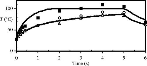
Figure 8. Tm:YAG laser thermal damage fields at t = 8 s. All four contours represent 63% damage (Ω = 1) for each damage process depicted. The innermost contour is collagen birefringence loss (a), the middle contour is muscle damage and disruption (b), the third contour is PC3 cell death from the two-state model (c), and the outermost contour is loss of clonogenicity in S-phase CHO cells according to the Mackey model, (d).

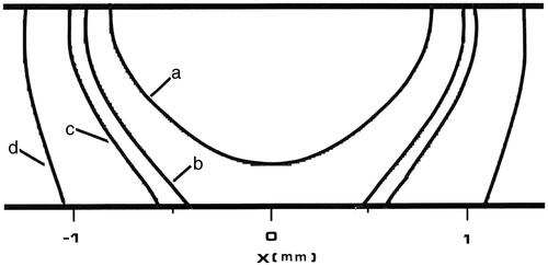
Table III. Summary of numerical model predictions of thermal damage (10% and 63% contours as indicated) for the Tm:YAG laser lesion at 5 and 50 s of heating. Calibration by collagen birefringence loss shows excellent agreement in this case for the thin tissue section. The damage/cell death bandwidth is indicated by 10–90% ΔR (mm).

Tm:YAG laser lesion (10% contours, except as noted)	Rmax (mm)	ΔR (mm)	Zmax (mm)	T (°C)
After 5 s of heating, 1 mm thick model.
Birefringence loss: Experiment, 63%	0.75		0.80	82
Model, 63%	0.81	0.14	0.84	80
After 5 s of heating, 2-mm thick model, 10%
PC3 cell death: Arrhenius calculation	1.08	0.35	0.99	60
Two-state calculation	1.08	0.14	1.05	60
CHO cell, probabilistic: G1-phase	1.18	0.05	1.09	55
S-phase	1.26	0.13	1.19	52
SN12 cell death [62]: Suspended cells	1.04	0.18	0.93	62
Attached cells	0.98	0.15	0.87	65
AT-1 cell death [72], apoptosis/necrosis	1.35	N/A	1.32	47
HepG2 cell death [82], attached cells	0.91	0.19	0.97	70
Micro-vascular disruption [66]	1.27	0.11	1.19	51
Muscle damage coefficients [65]	1.08	0.22	0.95	60
Skin burn coefficients [39]	1.18	0.21	1.09	55
After 50 s of heating, 2 mm thick, 10%
PC3 cell death: Arrhenius calculation	1.26	0.38	1.28	50
Two-state calculation	0.95	0.18	0.84	59
SN12 cell death [62]: Suspended cells	1.13	0.27	1.09	53
Attached cells	1.03	0.24	0.96	56
AT-1 cell death [72], apoptosis/necrosis	1.68	0.4	1.69	41
HepG2 cell death [82], attached cells	0.94	0.28	0.85	59
Micro-vascular disruption [66]	1.48	0.31	1.43	44.5
Muscle damage coefficients [65]	1.22	0.33	1.24	50
Skin burn coefficients [39]	1.20	0.14	1.21	51

Neither the HepG2 nor MRC-5 cell processes from the O’Neill model result in metabolic death above 0.2% in this model – they are both extremely slow processes in comparison to the others, even to collagen denaturation, which would completely overwhelm these two metabolic death processes. Interestingly, the Shah and Bhowmick Arrhenius coefficients for HepG2 cells predict predict a 10–90% transition zone of 0.19 mm located at r = 0.91 mm (Table III).

Contrary to what might have been expected, the Arrhenius calculation under-predicts the cell death with respect to the two-state model, as in Figure 9. This high temperature under-prediction is most likely due to the high temperature sensitivity of the two-state model, reflected in the much larger value of γR compared to E_a. After laser shut-off, the growth of the cell death and other process contours is negligible in both calculations.

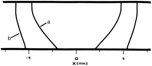
Figure 9. Tm:YAG laser PC3 cell death field at t = 8 s. Inner contour (a) is 63% cell death by the (slower) Arrhenius calculation (and corresponds to the 72 °C contour at 5 s) and the outer contour (b) is 63% cell death (Ω = 1) by the two-state model prediction (and corresponds to the 61 °C contour at 5 s).

Slower heating to temperatures near 90 °C

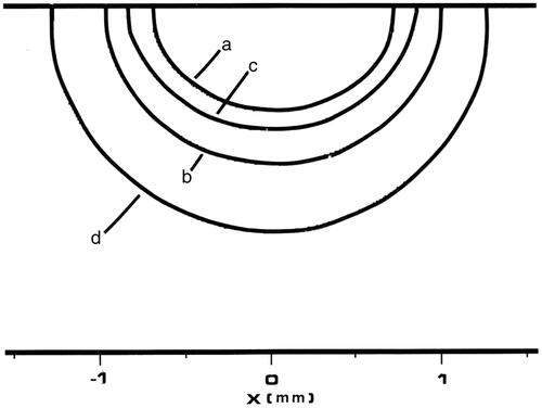
The longer heating time model with the Tm:YAG laser used the same Gaussian beam parameters at a slightly reduced power of 0.25 W for 50 s with 5 s of cooling. The top surface centre temperature reached 90 °C at t = 18 s, and sustained that temperature for the rest of the 50 s heating time (i.e. 90 °C for 32 s). The resulting 63% damage contours (Ω = 1) are shown in Figure 10. The contour designations used in Figure 8 have been retained in this plot. Note that the relative positions of the (b) (muscle damage) and (c) (PC3 two-state model) contours have reversed in this longer term heating. Just as for the shorter heating time, neither the HepG2 nor MRC-5 cell metabolic O’Neill et al. process models (at <0.09% death rate) will be observable outside of the boundary of severe coagulation represented by the collagen denaturation boundary. The Shah and Bhowmick [68] Arrhenius coefficients for HepG2 cells predict a 10–90% transition zone of 0.28 mm located at r = 0.94 mm (Table III).

Figure 10. Plot of damage process predictions from 50 s of Tm:YAG laser heating analogous to Figure 8. All four contours represent 63% damage (Ω = 1) for each damage process depicted, and the designations used in Figure 8 have been preserved. The innermost contour is collagen birefringence loss (a), the third contour is muscle damage and disruption (b), the second contour is PC3 cell death from the two-state model (c), and the outermost contour is loss of clonogenicity in S-phase CHO cells according to the Mackey model, (d). Note that the relative positions of contours (b) and (c) have reversed between the two figures.

Discussion

A review of the mathematical underpinnings and physical principles of thermal dose units, CEM, and Arrhenius damage integral predictions, C(τ), supports both approaches to the modelling and assessment of irreversible thermal alterations in tissues and cell culture within the framework of their governing assumptions: that the transformation consists of a single first-order single transition-state irreversible reaction (i.e. described by one dynamic state equation). CEM is an alternative weaker form of the Arrhenius formulation, designed to be used over a relatively narrow temperature range. The two predictions will essentially agree over the narrow range, and deviate as the temperature increases much above 48 °C, as described by Sapareto and Dewey [20]. For example, comparing Equations (1) and (9) it is easily seen that:

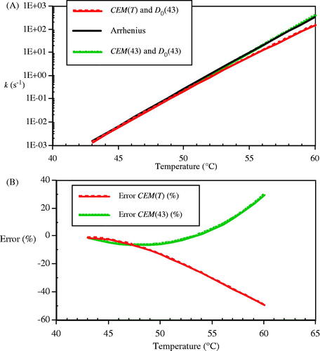
Figure 11 compares calculations of cell death rate by Equation (27b) for the CHO cells based on the temperature-dependent time scaling ratio, R_CEM(T) from Equation (4), and a constant time scaling ratio, R_CEM =R_CEM(43) = 0.477 (Table II) with the Arrhenius rate, k, for temperatures from 43–60 °C. The relative rates of increase agree well near 43 °C and deviate significantly at temperatures above 50 °C, as seen in Figure 11B. These calculations were made with perfectly matched coefficients, which give good agreement as long as the temperature is not too high. The rates of cell death would differ by orders of magnitude at all temperatures if the Arrhenius rate for the SN12 cells was compared to the single CEM calculation based on R_CEM = 0.5 – for example, at 43 °C a CEM calculation based on R_CEM = 0.5 overestimates the cell death rate for SN12 cells by a factor of 48, and at 60 °C it overestimates the cell death rate by a factor of 14 000.

Figure 11. Comparison of the predicted rates of loss in CHO cell clonogenicity by the CEM and Arrhenius approximations. A) Rate of loss of clonogenicity, k, calculated from the Arrhenius relation (solid line), by using temperature-dependent R_CEM(T) and D₀(43) = 697.7 s (- - -), and by R_CEM(43) = 0.477 and D₀(43) = 697.7 s (- • - • -). B) The errors in the two CEM approximations (%) referred to the Arrhenius rate (%); temperature-dependent R_CEM(T) (- - -) and R_CEM = 0.477 (- • - • -).

The Arrhenius formulation represents one of the founding pillars of physical chemistry, and has been successfully used for many decades to describe single reaction irreversible processes in structural proteins and some cell death processes. Thermal dose units effectively compare differing thermal histories to place them on a common ground for those cell death processes with similar time scaling ratios, R_CEM = 0.5, which is what they have been specifically designed to do, but do not provide a prediction of outcome. Further, only one number results, and so it is not possible to separate the differing effects of multiple parallel damage processes, each with different thermal response parameters, nor to determine their relative boundaries.

Analysis of thermal histories in terms of C(τ) allows separation of effects and the inclusion of multiple processes operating in parallel, but also has many additional advantages. Besides numerical model studies, the results can be readily and directly compared to any quantitative marker of thermal damage for which process coefficients are available: histological assay, vital stain intensity, fluorescence, enzyme histochemistry and the like. The outer and inner boundaries of transitional zones – anatomical and physiological changes that are grossly observable or observable as damage zones in images, such as MRI, US or CT imaging – are equally predictable from numerical models or measured spatio-temporal temperature fields. For example, the outer and inner boundaries of vascular haemorrhage in an ablation lesion can be predicted from the coefficients reported by Brown et al. [66] combined with a more severe coagulative process to delimit the inner boundary [11]. Severe changes in collagen can be predicted either in terms of the shrinkage [44–46] using the modified formulation described by Pearce [12] or can be used to predict the onset of collagen gellification, as is the desired end point in tissue fusion applications. Birefringence loss in muscle and in collagen is a convenient histological marker in higher temperature lesions [40,41,43]. Additionally, calculations of C(τ) can reveal underlying process characteristics that might not be obvious from the coefficients or from CEM₄₃ alone.

It must be borne in mind, however, that the standard CEM calculation describes only one type of thermal damage process: loss of clonogenicity under hyperthermic heating in some cell types. This has widely been hypothesised to be a combination of apoptosis [20,21,68], necroptosis [50,69], autophagy and necrosis [70]. However, these intrinsic cell death processes are actually complex functional protein cascades, typically consisting of multiple feedback loops describable by multi-component reactions and much higher-order systems of state–space equations, with far less obvious dynamic response [19]. It is, therefore, not surprising that single irreversible reaction Arrhenius models are not functionally sophisticated enough to accurately predict measured cell survival experimental data at lower temperatures characteristic of hyperthermia, especially in the earlier stages of heating where they usually over-predict cell death. The more functionally sophisticated multi-state models suggested by O’Neill et al. [17] and by Feng et al. [18] are capable of accurately representing the early stage shoulder region typically observed in cell survival experiments.

Comparison of damage and cell death processes

The probabilistic model developed by Mackey and Roti Roti accurately predicts clonogenicity loss in their CHO experiments, and is tractable for inclusion in numerical models. However, as Roti Roti notes [71], it is an exercise in curve fitting and was not obtained from fundamental thermodynamic analysis. Nevertheless, the model is strikingly accurate for those data. It is similar to the elegant biochemical model of Eissing et al. in that it includes stochastic population dynamics and a response delay feature. This suggests that new models of processes intending to describe the result of functional protein cascades – loss of clonogenicity, apoptosis and the like – should include features analogous to these in order to be successful.

Equally accurate predictions were obtained by the three-compartment model of O’Neill et al. [17], which fits their data extremely well for the two cell types studied. Their approach was seen to be equivalent to relaxing two of the governing assumptions in the classical Eyring/Arrhenius formulation yielding a reversible reaction with two dynamic state–space equations and achieving delay. This is a very illuminating observation, and indicates a potentially exciting avenue of investigation that should be pursued in future by investigators in this area.

The model applied by O’Neill et al. [17] achieves the delay by artificially expressing the Alive to Vulnerable velocity in a non-linear form: k_f = k_f0 e^T/Tk (1-A) – that is, the rate at which the vulnerable population appears is lowered by the (1-A) factor. A standard reversible reaction calculation from Equation (6) exhibits a somewhat similar dynamic response, as shown in Figure 12B. The extra delay built into the O’Neill model results in a sigmoidal decrease (i.e. showing a shoulder region) in the alive population, A, in Figure 12A that is not observed in the reversible reaction alive population, Figure 12B, which accounts for the differences in the vulnerable and dead cell population responses between the two models. Adding the non-linear forward velocity term as was done in the O’Neill et al. model is equivalent to including two association/dissociation reactions, indicated by the hypothetical [A][A] and [A][D] products in the modified dynamic response relations: where the forward velocity term does not include the (1-A) product and is indicated by the added ‘p’ subscript. Equations (28) are remarkably similar to Equations (12) in both style and construction. This revised form of the reversible reaction formulation now has the delay feature, as in the Eissing et al. [19] biochemical model for analogous reasons, and the shoulder region results from fundamental thermodynamic origins in this construct.

Figure 12. The dynamic response of A) the O’Neill et al. model at 90 °C and B) a comparison arbitrary reversible reaction model as in Equation (6) with constant coefficients of k_a = 0.007, k_b = 0.008 and k_c = 0.01 (s⁻¹).

Interestingly, the reversible reaction A population exhibits a simple exponential decrease, just as in the irreversible Arrhenius calculation. This suggests that a viability assay that measures the Alive population directly in a simple reversible reaction process may be well fitted by Arrhenius coefficients, while an assay that directly measures the dead cell population in the same experiment series might have a distinct shoulder region that requires a more sophisticated model. Approaches that utilise the reversible reaction form, with or without dissociation terms, should prove more effective than irreversible Arrhenius models when a survival curve has an observable shoulder region.

The two-transition-state equation thermodynamic model of Feng et al. [18] is almost as accurate for predicting cell survival curve measurements and is also attractive because of its fundamental thermodynamic origin. To date, the necessary coefficients have only been determined for PC3 cells. This two-state model is ‘faster’ than its Arrhenius equivalent (i.e. it has a higher equivalent to the activation energy), and usually has a narrower 10–90% cell death band.

The AT-1 Dunning rat prostate tumour model is very interesting because it has been studied with multiple methods. The AT-1 thermal damage process used in the numerical model work (Table III) consisted of a mixture of apoptosis and necrosis evaluated histologically [72]. The Arrhenius coefficients for this process given in Table II fit the original data quite accurately, and above the break point at 50 °C indicate a very slow process since the activation energy, E_a, is so low. That a single irreversible Arrhenius reaction is effective in the AT-1 tumour case suggests that the apoptosis/necrosis process may be engaged downstream of the intricate multi-component multi-step reversible state equations in the Eissing model – perhaps direct activation of one of more of the executioner caspases [19]. Thermally induced necrosis in the AT-1 tumour would not rely on the caspase cascade – it is not possible at this point to tell if the actual process might have been necroptosis – but, since the simple irreversible kinetics fit applies, whatever process has been activated may be modelled as a simple irreversible reaction. The same group also studied membrane injury indicated by calcein leakage and PI uptake, and included loss of clonogenicity in these cells in an earlier study [73]. The apoptosis/necrosis data are well fitted by the irreversible Arrhenius formulation [72], while the calcein leakage, PI and clonogenicity data show a significant shoulder region in the early stages of heating before a constant rate is established [73]. The error in the Arrhenius fit for these processes is significant. As an example, Figure 13 plots the reported data for calcein leakage against the Arrhenius prediction from coefficients that were determined at 30% loss in calcein signal: A = 5.069 × 10¹⁰ (s⁻¹) and E_a = 8.133 × 10⁴ (J mol⁻¹). As in Figure 6, the loss is substantially over-predicted in the early stages and the curve shape is incorrect. Other data in the ensemble show similar trends.

Figure 13. Plot of calcein signal loss in Dunning AT-1 tumour cell studies [73]. Data points were extracted from mean values in Figure 2 of the publication. The Arrhenius fit was based on reported parameters (lines as indicated). In both cases the signal loss is over-predicted except for the longest heating times.

Several apparently thermally robust cell types, such as the SN12 cells [62] among others, are very well fitted by the simpler single irreversible reaction Arrhenius kinetics. The particular damage/death processes that were studied constitute the defining realm in which the calculations apply. The damage process measured in the HepG2, MRC-5, PC3, SN12 and some of the AT-1 cells was loss of function indicated by vital stains. SN12 [62] and AT-1 [73] data were collected using fluorescent vital stains: PI (red fluorescent at 617 nm), which stains dead cells, and Hoechst 33342 (green fluorescent at 535 nm), which stains all cells. It is particularly interesting that for PI staining in the SN12 cells the simple irreversible Arrhenius calculation is effective and accurate, while for the same type of vital stain in the PC3 cells [18] it is not, because there is an obvious shoulder region. Plainly, different physical processes dominate for the two different cell types under the same vital stain. AT-1 cell death was also studied with EthD-1 (Ethidium homodimer-1), red fluorescent, indicating the nuclei of cells with compromised plasma membrane [72]. The particular dyes used in the HepG2 and MRC-5 study [17] were not specified, but the fluorescence was measured at 490 and 650 nm, and described as indicating metabolic cell death. In any event, those processes are extremely slow in nature and made no contribution in the laser exposures, even for the high temperatures reached.

To obtain a clear picture of the expected results it is essential to maintain several independent damage processes operating in parallel in numerical models, as has been done in the published results. Severe damage, such as substantial disruption in structural proteins or the vascular tree in ablation procedures, will always dominate histological observations and functional physiological imaging, and therefore dominate the observed tissue changes. Numerical model predictions need to be similarly graded and layered to be adequately representative of the expected results.

Relationship between Arrhenius model parameters

Finally, some consideration of the relationship between the Arrhenius coefficients is in order. In their landmark 1939 paper Eyring and Stearn [74] observed that the activation entropy, ΔS* = (ΔH* − ΔG*)/T, varied over a relatively small range in the food processing enzymes that they studied. Similarly, in 1971 Rosenberg et al. [75] demonstrated ‘compensation law’ behaviour between ΔS* and ΔH* for a large number of proteins: where T_c is the ‘compensation law’ temperature, 329 K (55.8 °C), and b = −271.7 (J mol⁻¹K⁻¹) in their study. They were perhaps among the first to suggest that irreversible protein alterations underlie all thermal damage processes.

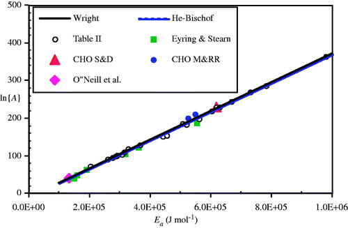
In 2003 two seminal papers appeared, one by Neil Wright [76] and the other by Xiaoming He and John Bischof [77] that demonstrated the strikingly linear relationship between ln{A} and E_a for multiple thermal damage processes studied to date. Wright used the ‘polymer in a box’ construct originally presented by Miles and Ghelashvili [78] to support the linear relationship hypothesis, and obtained the following fit line for multiple thermal damage process reports:

Nearly simultaneously in 2003, and in a follow-up recalculation with slightly different units [14], He and Bischof reported a similar correlation for a wider range of Arrhenius process damage coefficients:

Either linear correlation may be used to provide estimates of ln{A} for the many reports that contain only the process energy, E_a, or as a sort of ‘sanity check’ for experimentally derived coefficients. Incidentally, all of the enzyme processes contained in Eyring and Stearn’s 1939 paper [74] plot very closely along either of the two nearly identical correlations in Equations (30) – see Figure 14. All four of the above references are quite excellent papers on this topic and highly recommended.

Figure 14. Plot of coefficients from Table II (open circles) and Eyring and Stearns’ enzyme measurements (solid squares) compared to Equations (17a) (solid line) and (17 b) (dashed line, barely distinguishable). Also shown are the Sapareto and Dewey CHO cell (large solid triangle), Mackey and Roti Roti coefficients (solid circles), and Arrhenius coefficients for the O’Neill et al. data as calculated for this paper (large solid diamond at left end of plot).

Conclusion

The supporting evidence for both C(τ) and CEM Arrhenius thermal damage process models is strong as long as the framework of the assumptions is maintained: the governing reaction is single step and irreversible. Of the two possible approaches, a C(τ) calculation provides the most flexible and adaptable approach, and is much more generally applicable, especially at higher temperatures where multiple damage processes in structural proteins and large scale coagulation dominate the delicate and intricate functional protein cascades characteristic of intrinsic cell death processes at lower temperatures. The two methods amount to different expressions of the same theory; however, while an Arrhenius C(τ) result can be estimated from a CEM calculation, it is not advisable to do so because of the limited temperature range over which they agree even when well-matched as to the particular process. When other processes are modelled from a single CEM calculation, the damage accumulation rate may be incorrect by several orders of magnitude when R_CEM varies. Neither of these single irreversible reaction estimates is effective or sufficiently accurate to describe hyperthermic temperature range heating in the shoulder region of a typical cell survival curve due to their incomplete functional form: most often both clonogenicity and dye uptake assays require some sort of higher order approach, although there are exceptions, as in the differing PI results between SN12 and PC3 cells.

By relaxing the governing assumptions that result in the simple Arrhenius form of Equation (8) to include two and three thermodynamic states, or by providing probabilistic curve fitting that includes a delay feature, adequate functional behaviour can be obtained. Approaches based on fundamental thermodynamic principles are preferred, and both the O’Neill and Feng approaches have firm bases.

Plainly, multiple parallel damage processes must be included in numerical model work to obtain effective and useful results, and a C(τ) approach is the only one capable of following several processes in parallel. Additionally, the linear correlation between Arrhenius process coefficients provides a powerful tool in creating and testing models of thermal damage. Outcome predictions based on Arrhenius parameters should always be tested against the original experimental data to establish that the implied assumptions are indeed applicable.

Of course, it must always be borne in mind that in vitro experimental results in cell cultures are only approximately representative of tumours in situ and should not be applied uncritically to prediction of results. Tumours are notoriously inhomogeneous as to genetic make-up, even from site to site within metastases [79] and interact with the surrounding stroma in complex ways, particularly with respect to the micro-vasculature. Tumours adapt to inter-cellular contact, for example, to further their goals, completely disregarding contact inhibition and apoptosis-inducing signals [52]. The tumour extra-cellular matrix often consists of densely packed collagen, and the tumour is often at high interstitial pressure in the stroma, which must be maintained by some sort of capsular structure, or its equivalent. Cells in culture are homogeneous in make-up, kept at uniform local atmospheric pressure in the nearly complete absence of stroma, and have little to no interaction with the culture medium except to absorb and reject metabolic constituents. Cultures are usually not subjected to inter-cellular mechanical contact signals and responses. Consequently, we should expect differences between tumour cell behaviours in the two environments. In fact, the Austrian group [17,59--61] have noted significant differences in HepG2 cell with LX-1 cell behaviour between trans-well incubation and a co-culture model [60]. Cell culture is a powerful experimental design that permits us to separate variables and study cellular characteristics in a controlled environment in the absence of physiological responses and the body’s attempt at maintaining homeostasis. No other construct makes that possible in living systems. However, cells in culture do not constitute a tumour any more than a dish of transistors can function as a computer. It is the dynamic characteristics of the interacting components as a system that defines its function.

Numerical modelling of lesions allows further dissection of the relative importance of the various physical processes by providing direct access to their controlling parameters. Calculation of transient temperature fields alone is certainly not sufficient – useful models ought to predict tissue responses to adequately represent experiment analysis or to evaluate the effectiveness of new and/or existing modalities since heating time and the particular process under study are also dominantly important considerations.

Declaration of interest

The continuing vital support provided by the T.L.L. Temple Foundation is gratefully acknowledged. The author alone is responsible for the content and writing of the paper.

Acknowledgement

The kind assistance of Thomas Eissing in providing his Copasi numerical apoptosis model execution file is gratefully acknowledged. The author would also like to gratefully acknowledge the many helpful comments and literature suggestions provided by colleagues John Bischof, Neil Wright and Dieter Haemmerich.

References

- Dewey WC, Hopwood LE, Sapareto SA, Gerweek LE. Cellular responses to combinations of hyperthermia and radiation. Radiology 1977;123:463–74
- Sapareto SA, Hopwood LE, Dewey WC. Combined effects of X irradiation and hyperthermia on CHO cells for various temperatures and orders of application. Radiat Res 1978;73:221–33
- Sapareto SA. The biology of hyperthermia in vitro. In: Nussbaum GH, editor. Physical aspects of hyperthermia. New York, NY: American Institute of Physics; 1982. 1–16
- Henriques FC. Studies of thermal injury, V. The predictability and significance of thermally induced rate processes leading to irreversible epidermal injury. Arch Pathol 1947;43:489–502
- Henriques FC, Moritz AR. Studies of thermal injury in the conduction of heat to and through skin and the temperatures attained therein: A theoretical and experimental investigation. Am J Pathol 1947;23:531–49
- Moritz AR. Studies of thermal injury III. The pathology and pathogenesis of cutaneous burns: An experimental study. Am J Pathol 1947;23:915–34
- Moritz AR, Henriques FC. Studies in thermal injury II: The relative importance of time and surface temperature in the causation of cutaneous burns. Am J Pathol 1947;23:695–720
- Fugitt CH. A rate process theory of thermal injury. In: Weapons Effect Division, Armed Forces Special Weapons Project Report, AFSWP-606. Washington, DC; 1955, 43 pages
- Weaver JA, Stoll AM. Mathematical model of skin exposed to thermal radiation. Aerospace Med 1967;40:24–30
- Pearce JA, Thomsen S. Rate process analysis of thermal damage. In: Welch AJ, van Gemert MJC, editors. Optical-thermal response of laser-irradiated tissue. New York: Plenum; 1995. 561–606
- Diller KR, Valvano JW, Pearce JA. Bioheat transfer. In: Kreith F, editor. CRC handbook of thermal engineering. Boca Raton: CRC; 2000. 114–215
- Pearce JA. Models for thermal damage in tissues: Processes and applications. Crit Rev Biomed Eng 2010;38:1–20
- Thomsen SL, Pearce JA. Thermal damage and rate processes in biologic tissues. In: Welch AJ, van Gemert MJC, editors. Optical-thermal response of laser-irradiated tissue. 2nd ed. Dordrecht, Netherlands: Springer; 2011. 487–549
- He X, Bhowmick S, Bischof JC. Thermal therapy in urologic systems: A comparison of Arrhenius and thermal isoeffective dose models in predicting hyperthermic injury. J Biomech Eng 2009;131:745071
- Nadall SD, Arora MA, Schiffter HA, Coussios CC. On the applicability of the thermal dose cumulative equivalent minutes metric to the denaturation of bovine serum albumin in a polyacrylamide tissue phantom. In: Ebbini AS, editor. 8th international symposium on therapeutic ultrasound; 2009. Minneapolis, MN: American Institute of Physics; 2009. 205–9
- Mackey M, Roti Roti JL. A model of heat-induced clonogenic cell death. J Theor Biol 1992;156:133–46
- O’Neill DP, Peng T, Stiegler P, Mayrhauser U, Koestenbauer S, Tscheliessnigg K, et al. A three-state mathematical model of hyperthermic cell death. Ann Biomed Eng 2011;39:570–79
- Feng Y, Oden JT, Rylander MN. A two-state cell damage model under hyperthermic conditions: Theory and in vitro experiments. J Biomech Eng 2008;130:041016
- Eissing T, Conzelmann H, Gilles ED, Allgower F, Bullinger E, Scheurich P. Bistability analyses of a caspase activation model for receptor-induced apoptosis. J Biol Chem 2004;279:36892–7
- Sapareto SA, Hopwood LE, Dewey WC, Raju MR, Gray JW. Effects of hyperthermia on survival and progression of Chinese hamster ovary cells. Cancer Res 1978;38:393–400
- Lepock JR, Kruuv J. Thermotolerance as a possible cause of the critical temperature at 43° in mammalian cells. Cancer Res 1980;40:4486–8
- Shapiro HM. Practical flow cytometry. 4th ed. New York: Wiley-Liss; 2003
- Overgaard J. Effect of hyperthermia on malignant cells in vivo. A review and a hypothesis. Cancer 1977;39:2637–46
- Leith JT, Miller RC, Gerner EW, Boone ML. Hyperthermic potentiation: Biological aspects and applications to radiation therapy. Cancer 1977;39:766–79
- Ross-Riveros P, Leith JT. Response of 9L tumor cells to hyperthermia and X irradiation. Radiat Res 1979;78:296–311
- Dewhirst MW, Viglianti BL, Lora-Michiels M, Hanson M, Hoopes PJ. Basic principles of thermal dosimetry and thermal thresholds for tissue damage from hyperthermia. Int J Hyperthermia 2003;19:267–94
- Arrhenius S. Uber die Reaktionsgeschwindigkeit bei der Inversion von Rohrzucker durch Sauren (On the reaction rate in the inversion of cane sugar by acids). Z Phys Chem 1889;4:226–48
- Johnson FH, Eyring H, Stover BJ. The theory of rate processes in biology and medicine. New York: Wiley; 1974
- Arrhenius S. Quantitative laws in biological chemistry. London: Bell; 1915
- Yarmolenko PS, Moon EJ, Landon C, Manzoor A, Hochman DW, Viglianti BL, et al. Thresholds for thermal damage to normal tissues: An update. Int J Hyperthermia 2011;27:320–43
- Pearce JA. Relationship between Arrhenius models of thermal damage and the CEM 43 thermal dose. Energy-based treatment of tissue and assessment V. Proc SPIE 2009;718104:1–15. doi:10.1117/12.807999
- Eyring H, Gershinowitz H, Sun CE. The absolute rate of homogeneous atomic reactions. J Chem Phys 1935;3:786–96
- Wynne-Jones WFK, Eyring H. The absolute rate of reactions in condensed phases. J Chem Phys 1935;3:492–502
- Laidler KJ, King MC. The development of transition-state theory. J Chem Phys 1983;87:2657–64
- Eyring H, Polyani M. Über Einfache Gasreaktionen (On simple gas reactions). Z Phys Chem B 1931;12:279–311
- Eyring H. The activated complex in chemical reactions. J Chem Phys 1935;3:107–15
- Maron SH, Lando JB. Fundamentals of physical chemistry. New York: Macmillan; 1974
- Eyring H. The energy of activation for bimolecular reactions involving hydrogen and the halogens, according to quantum mechanics. J Am Chem Soc 1931;53:2537–49
- Diller KR, Klutke GA. Accuracy analysis of the Henriques model for predicting thermal burn injury. In: Roemer, RB, editor. Advances in bioheat and mass transfer. New York: ASME; 1993. 117–23
- Thomsen S, Pearce JA, Cheong WF. Changes in birefringence as markers of thermal damage in tissues. IEEE Trans Biomed Eng 1989;36:1174–9
- Pearce JA, Thomsen SLMD, Vijverberg H, McMurray TJ. Kinetics for birefringence changes in thermally coagulated rat skin collagen; Los Angeles, CA. Bellingham, WA, USA: Proc. Society of Photo-Optical Instrumentation Engineers; 1993. 180–6
- Maitland DJ, Walsh JT Jr. Quantitative measurements of linear birefringence during heating of native collagen. Lasers Surg Med 1997;20:310–18
- Pearce JA, Thomsen S. The effect of vessel architecture on fusion by radio frequency current. surgical applications of energy. San Jose, CA: SPIE; 1998. 217–28
- Chen SS, Wright NT, Humphrey JD. Heat-induced changes in the mechanics of a collagenous tissue: Isothermal free shrinkage. J Biomech Eng 1997;119:372–8
- Chen SS, Wright NT, Humphrey JD. Heat-induced changes in the mechanics of a collagenous tissue: Isothermal, isotonic shrinkage. J Biomech Eng 1998;120:382–8
- Chen SS, Wright NT, Humphrey JD. Phenomenological evolution equations for heat-induced shrinkage of a collagenous tissue. IEEE Trans Biomed Eng 1998;45:1234–40
- Pearce JA. Corneal Reshaping by Radio Frequency Current: Numerical Model Studies. Thermal Treatment of Tissue: Energy Delivery and Assessment. Proc SPIE 2001;4247:109–18. doi:10.1117/12.427850
- Alberts B, Johnson A, Lewis J, Raff M, Roberts K, Walter P. Molecular biology of the cell. 5th ed. New York: Garland Science; 2008
- Vanden Berghe T, Vanlangenakker N, Parthoens E, Deckers W, Devos M, Festjens N, et al. Necroptosis, necrosis and secondary necrosis converge on similar cellular disintegration features. Cell Death Diff 2010;17:922–30
- Vandenabeele P, Galluzzi L, Vanden Berghe T, Kroemer G. Molecular mechanisms of necroptosis: An ordered cellular explosion. Nature Rev Mol Cell Biol 2010;11:700–14
- Wrighton KH. Cell death: A killer puts a stop on necroptosis. Nat Rev Mol Cell Biol 2011;12:279
- Weinberg WA. The biology of cancer. New York: Garland Science; 2007
- Zhang Y, Calderwood SK. Autophagy, protein aggregation and hyperthermia: A mini-review. Int J Hyperthermia 2011;27:409–14
- Bergsbaken T, Fink SL, den Hartigh AB, Loomis WP, Cookson BT. Coordinated host responses during pyroptosis: Caspase-1-dependent lysosome exocytosis and inflammatory cytokine maturation. J Immunol 2011;187:2748–54
- Mathews CK, van Holde KE, Appling DR, Anthony-Cahill SJ. Biochemistry. 4th ed. Toronto: Pearson; 2013
- Deveraux QL, Reed JC. IAP family proteins – Suppressors of apoptosis. Genes Dev 1999;13:239–52
- Wright NT. Parameter Correlation in Models of Hyperthermic Cell Death. American Society of Mechanical Engineers 2011 Summer Bioengineering Conference, Farmington, PA, June 2011. New York: ASME; 2011. pp SBC2011–53933
- Stiegler P. Vital stains used in HepG2 and MRC-5 experiments. Personal communication, 2012
- Mayrhauser U, Stiegler P, Stadlbauer V, Koestenbauer S, Leber B, Konrad K, et al. Effect of hyperthermia on liver cell lines: Important findings for thermal therapy in hepatocellular carcinoma. Anticancer Res 2011;31:1583–8
- Mayrhauser U, Stiegler P, Stadlbauer V, Koestenbauer S, Leber B, Konrad K, et al. Cell to cell interactions influence sensitivity of liver cell lines during hyperthermia. Anticancer Res 2011;31:3713–7
- Leber B, Mayrhauser U, Leopold B, Koestenbauer S, Tscheliessnigg K, Stadlbauer V, et al. Impact of temperature on cell death in a cell-culture model of hepatocellular carcinoma. Anticancer Res 2012;32:915–21
- He X, Bischof JC. The kinetics of thermal injury in human renal carcinoma cells. Ann Biomed Eng 2005;33:502–10
- Feng Y, Fuentes D. Model-based planning and real-time predictive control for laser-induced thermal therapy. Int J Hyperthermia 2011;27:751–61
- Pearce JA, Cilesiz I, Welch AJ, Chan EK, McMurray TJ, Thomsen SLMD. Comparison of Ho:YAG, Tm:YAG, and argon lasers for fusion of intestinal tissues. Bellingham, WA: Proc. Society of Photo-Optical Instrumentation Engineers, 1994. Volume 2128, pp 517–26
- Jacques SL, Gaeeni MO. Thermally induced changes in optical properties of heart. IEEE Eng Med Biol Mag 1989;11:1199–200
- Brown SL, Hunt JW, Hill RP. Differential thermal sensitivity of tumour and normal tissue microvascular response during hyperthermia. Int J Hyperthermia 1992;8:501–4
- Cooper TE, Trezek GJ. Correlation of thermal properties of some human tissues with water content. Aerospace Med 1971;42:24–7
- Wust P, Hildebrandt B, Sreenivasa G, Rau B, Gellermann J, Riess H, et al. Hyperthermia in combined treatment of cancer. Lancet Oncol 2002;3:487–97
- Eriksson JE, Vandenabeele P. Workshop summary: Cell death mechanisms controlled by the TNF family. Adv Exp Med Biol 2011;691:585–8
- Thomsen SL. The art and science of low-energy applications: pathology perspectives. Proc. Thermal Treatment of Tissue: Energy Delivery and Assessment VI. San Francisco, CA. Bellingham, WA: Society of Photo-Optical Instrumentation Engineers, 2011. Article no.: 790102
- Roti Roti JL. Cellular responses to hyperthermia (40–46 °C): Cell killing and molecular events. Int J Hyperthermia 2008;24:3–15
- Bhowmick S, Swanlund DJ, Bischof JC. In vitro thermal therapy of AT-1 Dunning prostate tumours. Int J Hyperthermia 2004;20:73–92
- Bhowmick S, Swanlund DJ, Bischof JC. Supraphysiological thermal injury in dunning AT-1 prostate tumor cells. J Biomech Eng 2000;122:51–9
- Eyring H, Stearn AE. The application of the theory of absolute reaction rates to proteins. Chem Rev 1939;24:253–70
- Rosenberg B, Kemeny G, Switzer RC, Hamilton TC. Quantitative evidence for protein denaturation as the cause of thermal death. Nature 1971;232:471–3
- Wright NT. On a relationship between the Arrhenius parameters from thermal damage studies. J Biomech Eng 2003;125:300–4
- He X, Bischof JC. Quantification of temperature and injury response in thermal therapy and cryosurgery. Crit Rev Biomed Eng 2003;31:355–421
- Miles CA, Ghelashvili M. Polymer-in-a-box mechanism for the thermal stabilization of collagen molecules in fibers. Biophys J 1999;76:3243–52
- Gerlinger M, Rowan AJ, Horswell S, Larkin J, Endesfelder D, Gronroos E, et al. Intratumor heterogeneity and branched evolution revealed by multiregion sequencing. N Engl J Med 2012;366:883–92
- Beckham JT, Wilmink GJ, Mackanos MA, Takahashi K, Contag CH, Takahashi T, et al. Role of HSP70 in Cellular Thermotolerance. Lasers Surg Med 2008;40:704–15
- Borrelli MJ, Thompson LL, Cain CA, Dewey WC. Time–temperature analysis of cell killing of BhK cells heated at temperatures in the range of 43.5 °C to 57.0 °C. Int J Radiat Oncol Biol Phys 1990;19:389–99
- Shah B, Bhowmick S. Evaluation of important treatment parameters in supraphysiological thermal therapy of human liver cancer HepG2 cells. Ann Biomed Eng 2006;34:1745–57
- Lepock JR, Frey HE, Bayne H, Markus J. Relationship of hyperthermia-induced hemolysis of human erythrocytes to the thermal denaturation of membrane proteins. Biochim Biophys Acta 1989;980:191–201
- Przybylska M, Bryszewska M, KedzioraKedziora J. Thermosensitivity of red blood cells from Down’s syndrome individuals. Bioelectrochemistry 2000;52(2):239–49