Generalised polynomial chaos-based uncertainty quantification for planning MRgLITT procedures

Abstract

Purpose: A generalised polynomial chaos (gPC) method is used to incorporate constitutive parameter uncertainties within the Pennes representation of bioheat transfer phenomena. The stochastic temperature predictions of the mathematical model are critically evaluated against MR thermometry data for planning MR-guided laser-induced thermal therapies (MRgLITT). Methods: The Pennes bioheat transfer model coupled with a diffusion theory approximation of laser tissue interaction was implemented as the underlying deterministic kernel. A probabilistic sensitivity study was used to identify parameters that provide the most variance in temperature output. Confidence intervals of the temperature predictions are compared to MR temperature imaging (MRTI) obtained during phantom and in vivo canine (n = 4) MRgLITT experiments. The gPC predictions were quantitatively compared to MRTI data using probabilistic linear and temporal profiles as well as 2-D 60 °C isotherms. Results: Optical parameters provided the highest variance in the model output (peak standard deviation: anisotropy 3.51 °C, absorption 2.94 °C, scattering 1.84 °C, conductivity 1.43 °C, and perfusion 0.94 °C). Further, within the statistical sense considered, a non-linear model of the temperature and damage-dependent perfusion, absorption, and scattering is captured within the confidence intervals of the linear gPC method. Multivariate stochastic model predictions using parameters with the dominant sensitivities show good agreement with experimental MRTI data. Conclusions: Given parameter uncertainties and mathematical modelling approximations of the Pennes bioheat model, the statistical framework demonstrates conservative estimates of the therapeutic heating and has potential for use as a computational prediction tool for thermal therapy planning.

• Bioheat transfer
• generalised polynomial chaos
• laser tissue interaction
• treatment planning
• uncertainty quantification

Introduction

Magnetic resonance-guided laser-induced thermal therapy (MRgLITT) is a minimally invasive ablative procedure that can rapidly (<180 s) deliver heat to treat focal cancerous lesions or radiation necrosis in the brain [1,2]. The optical fibre is placed through a burr hole into the target disease via stereotaxy, analogous to an image-guided stereotactic biopsy [1,3]. MRgLITT for patient-specific treatment of focal cancerous lesions in brain presents an attractive treatment option with significantly less impact on the patient compared to conventional surgical procedures. For many anatomical sites of interest, magnetic resonance image (MRI) guidance provides a means for planning, targeting, monitoring and verifying the delivery of these therapies in a single, closed-loop session. To this end, several FDA-cleared MRgLITT systems (Monteris www.monteris.com, Visualase www.visualaseinc.com) have become commercially available. These systems facilitate MRgLITT procedures on any modern clinical MRI scanner and are currently in post-market studies at multiple institutions [1,3–9]. The goal of the therapy is to treat a targeted tissue volume, < 3 cm in diameter, in such a highly controlled manner so as not to incur damage to nearby normal tissue structures which would result in complications.

Proton resonance frequency-based thermometry or magnetic resonance temperature imaging (MRTI) provides a means to real-time monitor the heat distribution during the therapy [10,11]. MRTI’s temperature information improves the safety and efficacy of MRgLITT by allowing the physician to avoid overheating, tissue vaporisation, and charring near the laser and prevent treating tissue beyond disease extent. However, in the current paradigm, visual assessment of multiple structures in multiple planes, even with the aid of user-assigned critical monitoring points, presents a delivery paradigm that is inherently difficult to manage. Integration of mathematical modelling and computational science techniques with the clinical imaging information available may prove useful for MRgLITT before and during the procedure, either by predicting the result of a treatment before the surgery, or during surgery to improve MRTI and robustly estimate lost information due to data corrupting motion, low signal-to-noise-ratio (SNR), excessive heating, and catheter-induced signal voids [12–15]. These enhanced real-time monitoring approaches may further assist in more safely and accurately controlling therapy delivery for increased efficacy of the procedure [16,17]. The availability of increasingly powerful high performance and portable computing resources, such as NVIDIA® graphics processing units (GPUs) [18] and Intel® many integrated core (MIC) architecture [19], indicates that the presence of computational science is likely to continue escalating in these image-guided thermal therapy procedures.

The development of computational tools for planning hyperthermia and ablation therapies has received significant attention for improving therapy outcomes [10,20–24]. With predictive modelling, the laser fibre placement can be planned in a virtual environment to improve the likelihood of a successful and short treatment. A common method for predictive modelling of the distribution of induced heating in blood perfused tissue is the Pennes bioheat transfer equation (BHTE) [25] solved with a finite element method (FEM) [26–28]. A difficulty in obtaining accurate results from the BHTE is the uncertainty incurred by using homogeneous literature values of biothermal and optical constitutive values for patient-specific planning. Uncertainty is further increased with incorporating the additional complexity of investigating the non-linear effects of temperature-dependent or thermal dose-dependent constitutive parameters.

Truly predictive prospective computer modelling requires substantial validation efforts and novel computer modelling techniques that incorporate the inherent uncertainties of the computer model into the predicted solution [29–31]. Monte Carlo modelling is the quintessential example of incorporating uncertainty into the computer model output. While a Monte Carlo approach would provide the necessary probabilistic outputs, the computational cost required to simulate a sufficient number of realisations is large. There exist methods to improve the convergence of Monte Carlo through the quasi-Monte Carlo method, Latin hypercube sampling, and the Markov Chain Monte Carlo method [32–36].

Another successful technique to accelerate uncertainty quantification (UQ) is generalised polynomial chaos (gPC) expansion. gPC provides a means of providing the model with UQ prodigiously faster than Monte Carlo for computations using few random input variables, i.e. <10 variables. gPC is originally based on the work of Wiener [37]. This method used a high order Hermite polynomial as a spectral approximation for model outputs. Nearly 50 years later, Ghanem and Spanos identified the spectral approximation as a viable tool in FEM modelling of stochastic differential equations [38]. Xiu and Karniadakis demonstrated that the convergence of spectral methods for solutions to differential equations were optimised by matching certain input functions’ distributions with corresponding output polynomials, known as the Wiener–Askey scheme [39]. For similar diffusive type equations, gPC’s convergence to a mean solution, N < 10 realisations, compares exceptionally favourably, pointwise error <1.E-2, when compared with Monte Carlo’s N = 20 000 realisations [39,40]. gPC has already been applied to an eclectic list of studies. The topics include radiation oncology, combustion modelling, nuclear reactor design, and robotic dynamics on rugged terrain [41–44].

Here we investigate the use of a stochastic form of the BHTE coupled to a diffusion theory approximation of light transport in tissue for improving the decision-making utility of thermal modelling. Temperature-dependent constitutive values are mathematically characterised via an assumed probability distribution providing the ability to perform uncertainty quantification via generalised polynomial chaos and provide quantitative confidence levels in the computer model predicted temperature for each spatial location at each time point.

Methods

Mathematical model of uncertainty

Ignoring discretisation errors, computer implementations of mathematical models fundamentally have uncertainty in their representation and predictions of physical phenomena [45] due to two dominant sources of inherent variability. (1) Simplifications are needed to make the algorithm practical. For example, in this work we employ a Pennes bioheat transfer equation (Equation 1) with a perfusion term that represents the manifestation of a complex and tortuous microvasculature on the bulk continuum scale heat transfer. (2) The computer model parameters are not known precisely. In this application, optical and biothermal parameters are taken from literature values and are empirical representations of non-linear temperature and damage-dependent phenomena. Further, the parameters fail to incorporate patient- and tissue-specific variability resulting from heterogeneities.

This investigation aims to manage model parameter uncertainty associated with a stochastic form of Pennes bioheat transfer equation for blood perfused tissues (Equation 1). The motivating idea is that the Pennes’ representation of the physics of the bioheat transfer phenomena coupled with statistical methods of uncertainty quantification may synergistically provide a reliable prediction model regardless of constitutive parameter uncertainties and mathematical modelling approximations.

Here, ρ is the tissue density, c_p is the specific heat of tissue, k, is the tissue conductivity; ω is the tissue micro perfusion primarily due to capillaries, c_blood is the specific heat of blood, and u_a denotes the arterial core blood temperature. The laser source term, q_laser, is modelled using a standard diffusion approximation [28]. Power is denoted P, the volume of applicator is denoted U_tip, and the volume of the biological domain is denoted U. Optical parameters include the absorption, scattering, and anisotropy factor, denoted μ_a, μ_s, and g, respectively. Arrhenius damage model, Ω, parameters are denoted, A, E_A, and R. The objective of this work is to use this mathematical model to predict the 4D temperature field, u, as a function of a random vector, , with a known probability distribution that mathematically represents our uncertainty the optical parameters, perfusion, and conduction, .

Statistical methods provided by uncertainty quantification techniques such as generalised polynomial chaos provide novel methodologies for modelling the complex bioheat transfer phenomena. In particular, it is well known that the constitutive parameters behave non-linearly with temperature increase and tissue damage. Constitutive parameters that account for damage-dependent non-linearities of the perfusion, thermal conductivity, and optical parameters [46] are generally more scarce than the linear counterparts and the variability of the mathematical form of the constitutive non-linearities seen within the literature suggests a potentially higher degree of uncertainty within the non-linear parameters [10,23,27,47,48]. Here we will consider the uncertainty associated with both linear and non-linear constitutive forms of the perfusion, absorption, and scattering. A goal of our work is to investigate if a relatively simple linear model with physically meaningful bounds on constitutive values can be coupled with stochastic methods to produce useful predictions. Stochastic parameters associated with linear forms of the BHTE are chosen by the following expressions that are spatially homogenous and constant in time.

While several empirical models of non-linearites are available, for feasibility, a common form of the constitutive non-linearities (Equation 3) was considered for absorption, scattering, and perfusion as a function of Arrhenius thermal damage, Ω. As seen in Figure 1, for this particular analytical form chosen [27], undamaged constitutive values transition to coagulated values between the temperature range of 51–61 °C. Similar to previous studies [49] of the time–temperature histories relevant to MRgLITT, the tissue is fully damaged at a threshold of approximately 61 °C.

Figure 1. A graphical illustration of the non-linear constitutive model [27] used for the perfusion and optical absorption is shown. The scattering behaves similar to the absorption. Damage, perfusion, and absorption are plotted as a function of a time–temperature history representative of those observed in MRgLITT procedures. As shown, the native undamaged constitutive values transition into coagulated constitutive values between temperatures of approximately 51–61 °C. Similar to previous results [49], the tissue is fully damaged at a threshold of 61 °C.

The native conduction, , perfusion, , optical scattering, , optical absorption, , and the optical anisotropy, as well as the coagulated values of the absorption, , scattering, ,and perfusion, , are understood mathematically as uniform random variables with quantitative bounds given in Table I. As seen in Figure 1, the uncertainty range of constitutive non-linearities is considered as a subset of the uncertainty within the linear UQ problem.

Table I. Literature-based constitutive values [46,50–52,54,55, 77–80] A table of the constitutive values used for perfusion, conduction, absorption, and scattering is shown. Uniform distributions are denoted U(a,b). Deterministic values are otherwise used. Values for density, specific heat, and Arrhenius parameters are as follows: ρ = 1045 (kg/m³), c_blood = 3840 (J/kg/K), c_p = 3600 (J/kg/K), A = 3.1E98 (1/s), E_A = 6.28E5 (J/mol), R = 8.314 (J/mol/K).

Figure	ω[kg/(m^3× s)]	k[W/(m × K)]	μa (1/m)	μs (1/m)	g (Unity)
2A	U (3, 9)	0.527	500	14000	0.88
2A	6	U (0.490, 0.527)	500	14000	0.88
2A	6	0.527	U (400, 600)	14000	0.88
2A	6	0.527	500	U (11200, 16800)	0.88
2A	6	0.527	500	14000	U (0.88, 0.95)
2B	6	0.527	Linear U (50, 600)	14000	0.88
2B	6	0.527	Native U (50, 300) Coag. U (300, 600)	14000	0.88
2B	6	0.527	500	Linear U (5000, 50000)	0.88
2B	6	0.527	500	Native U (5000, 30000) Coag. U (30000, 50000)	0.88
2C	Linear U (0, 9)	0.527	500	14000	0.88
2C	Native U (3, 9) Coag. U (0, 3)	0.527	500	14000	0.88
2D	U (3, 9)	U (0.490, 0.527)	U (400, 600)	U (11200, 16800)	0.88
3	0	0.527	U (4, 200)	U (11200, 16800)	U (0.85, 0.95)
4, 5, 6	6	0.527	U (400, 600)	U (11200, 16800)	U (0.88, 0.95)
5A (WM)	U (3, 9)	0.527	320	46900	0.88

Coag, coagulated; WM, white matter.

Constitutive data

Constitutive parameter values [46,50–55] used in simulating the bioheat transfer for the in vivo brain data and ex vivo phantom set-up are provided in Table I. Variability in the model parameters [46,55,56] was input into the gPC model as uniformly distributed random variables using the bounds shown in Table I. The variability in the ranges presented encompasses all conceivable healthy values as well as the extremum of constitutive non-linear dependence on temperature. The values for the Arrhenius dose parameters listed in Table I are from Henriques and Moritz’s classic work [57]. The choice of dose parameters is dependent on what end point is sought. Here the threshold is tissue death by any heating effects shortly (<20 min) after treatment. The dose analysis for the four canines, described by Yung et al. [49], demonstrates that an Arrhenius dose module using Henriques’ dose values leads to agreement with post-treatment, post-contrast T1-weighted MRI.

Optical parameter uncertainty

Relatively large variability may be seen in optical parameter values reported in the literature, Table I. These differences may be associated with different techniques for in vivo and in vitro measurements, different radiative transport models, and differences in preparation of tissue specimens [58,59]. The non-linear behaviour of optical parameters is well known [27,46,60–62] and further increases the uncertainties in optical properties. For example, a 10% increase in the absorption coefficient and a 2–4-fold increase in the scattering coefficient was seen between native and coagulated brain tissue [46,61]. Further, the blood content of the tissue has been seen to affect the optical properties [63]. Significant changes in the optical properties of the blood can be expected with varying concentrations of haematocrit and oxygen concentration. There is also great uncertainty in the tumour type to use for the optical parameter values as well as blood content of the tumour. This may particularly contribute to the uncertainty in the optical parameters when irradiating heterogeneous tumours where the patient-specific blood content and the amount of cerebral spinal fluid (CSF) present may vary significantly.

Grey matter optical parameter values – μ_a, μ_s, and g – were used in simulating MRgLITT in normal canine brain tissue. For non-linear simulations, the values of absorption and scattering were set to represent the native state and transition to a coagulated state (Equation 3). The range of optical values used in the linear simulation for comparison against the non-linear simulation is a superset of the range of the native and coagulated transition, listed in Table I, Figure 2(B) and (C).

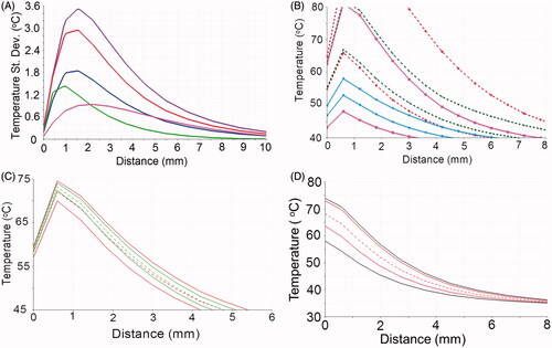
Figure 2. These plots are spatial profiles that demonstrate the properties of a stochastic BHTE, with inputs listed in Table I. A is a linear sensitivity study; each colour represents data from a univariate model, i.e. one parameter is varied while all others are constant. A has the following plots, listed from low to high variance at peak heating: perfusion (fuchsia), conductivity (green), optical scattering (blue), optical absorption (red), and optical anisotropy (violet). The parameters’ relative sensitivities can be seen in this figure. For example, perfusion is proportionally varied more than the optical absorption and scattering parameters, but the optical parameters still have a greater temperature variance. The BHTE is most sensitive to the anisotropy factor in this study. B and C are a sensitivity study comparing linear and non-linear perfusion parameters; For B and C, the solid lines represent the CDF = 2.3 and 97.7%; the enclosed region is the central 95% confidence interval. B has optical absorption (red and green with dashed lines) and scattering (fuchsia and blue with solid lines) while C has perfusion. The linear cases’ inputs vary the concerned parameter over a range that includes both the native and coagulated states of the non-linear case. The plots demonstrate coagulation affecting the temperature distributions. D simultaneously varies optical scattering, optical absorption, conductivity, and perfusion. The difference between the worst-case scenarios (black) and CDF = 1% and 99% (red) is shown.

Multiplanar magnetic resonance thermal imaging in phantom and animal models

Simulations were compared to MRTI data obtained from a safety and feasibility study of MRgLITT conducted in the brains of four clinically normal mixed breed hounds (20–25 kg) [28,49]. MRTI data was also obtained from an MRgLITT heating experiment in a perfusionless ex vivo tissue phantom [17] constructed from an excised canine prostate embedded within 1% agar, Figure 3. MRTI data was acquired on a 1.5 T MRI scanner (ExciteHD®, GE Healthcare Technologies, Waukesha, WI) with an 8-channel, receive-only phased array head coil (MRI Devices, Gainesville, FL) and a 2D multi-slice 8-shot EPI sequence [64] (flip angle (FA) = 60°, field of view (FOV) = 20 × 20 cm, slice thickness 4 mm, TR/TE = 544/20 ms, encoding matrix of 256 × 128, with 5–6 s per update). The procedures were conducted under institutional protocol. The canines were anaesthetised with ketamine/midazolam (Versed) solution (ketamine, 10 mg/kg; midazolam, 0.5 mg/kg; and glycolpyrrolate, 0.01 mg/kg), incubated, and aspirated with a mixture of 2% isoflurane/oxygen. Once the dogs were anaesthetised, a burr hole was introduced in the right parietal bone of each animal. In each case, the laser applicator was percutaneously placed through the burr hole and into the clinically normal brain. The silica applicator was 400 μm in diameter with a 1-cm axial length for laser diffusion. The laser wavelength was 980 nm with a maximum power of 15 W (Photex 15, BioTex, Houston, TX). The applicator was water cooled with a maximum flow of 15 mL/min. Power histories are shown in Figures 3 and 4. Flouroptic probes were not included to attempt to avoid susceptibility artefact.

Figure 3. The trivariate joint uncertainty of the optical absorption, scattering, anisotropy are input for the gPC simulations. Model parameters are listed in Table I. A is the MRTI of the phantom study at t = 90 s. The inner red contour is the 50 °C isotherm for the model’s mean and the outer red contour is for the CDF = 97.3%; CDF = 2.3% never reaches 50 °C. The dark blue contour is the MRTI’s 50 °C isotherm. Only one MRTI isotherm is displayed because the MRTI variance is very small; ± 2σ of MRTI noise is ∼2 °C. The black rectangles in A, B, and D occlude where the laser fibre was. The superimposed green line represents the location for linear profiles B and D. A green diamond indicates the location of the temporal profile in C. D compares the linear profile of the central 95% confidence intervals of the model and MRTI. In plot D, the model’s mean tracks very well with the MRTI, particularly near the laser fibre (±∼6 mm). D also dramatically shows the potential for non-Gaussian distributions to arise in the temperature model, further illustrated in B. B shows various CDF values tracked in the gPC computer package, DAKOTA. The top red is CDF = 99%, green is the median (50%), red dashed line is the mean, violet is 5%, black is 2.3%, bottom red is 1%. Note the extreme skewness of the model’s temperature output near the fibre, as evidenced by the mean and median being much nearer the higher percentage CDFs than the lower percentage CDFs. The power, displayed as green points, is provided units on the right vertical axis of C.

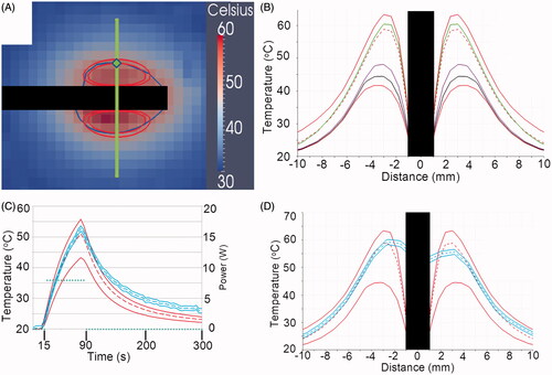
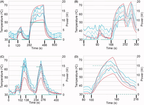
Figure 4. These temporal profiles, A through D, are temporal profiles from canines 1 through 4, respectively. The red and blue dashed and solid lines represent the same mean and CDF values listed in Figure 5. The green points represent the power history. The spatial locations of the temporal profiles are shown in Figure 6 via the green diamonds. A and D show the best agreement of the four plots. B is more successful at the beginning of the imaging sequence but the model is much colder at later time points. C tends to be somewhat cooler, but significant overlap remains between the MRTI and model distributions.

Computational methods

A hexahedral finite element mesh that conforms to the geometric details of the water cooled laser applicator [28,65] was created in CUBIT (Sandia National Laboratories, Albuquerque, NM) [66]. A 21 °C Dirichlet boundary condition representing the water-cooled catheter was applied to the domain of the applicator. Simulations at several mesh spatial resolutions were run at quarter symmetry to ensure numerical convergence; 13968/47368/169680 element meshes with 15770/50898/177549 corresponding nodes were evaluated. The DAKOTA software (Sandia National Laboratories) [67] was used to implement the generalised polynomial chaos expansion. Similar to ensuring convergence of the mesh resolution, the number of polynomial chaos basis functions used in the gPC expansion was increased until the truncation error of the gPC expansion was negligible [68]. This was achieved by computing the difference between a lower order and a higher order gPC expansion. When the maximum pointwise difference between a lower order and a higher order gPC expansion was <0.001 °C, the gPC expansion was assumed converged. Using DAKOTA, the gPC expansion order is inferred from the quadrature order in probability space. A quadrature order of four was found to achieve truncation error convergence in the gPC expansion. For comparison to gPC, a worst-case scenario approach was also run [69]. The worst-case scenario approach provides the extreme upper and lower bound of the temperature distribution by considering the extrema of the input parameter variability.

Results

A sensitivity study of the thermal conduction, perfusion, absorption, scattering, and anisotropy is presented in Figure 2. The sensitivity study was performed by investigating the effect of the uncertainty range of each parameter individually on the resulting temperature field’s standard deviation (Figure 2A) or mean and 95% confidence interval (Figure 2B–D). Here the 95% confidence intervals are reported as the output cumulative temperature distribution (CDF) between 2.5% and 97.5%. Representative profiles of the temperature field’s standard deviation resulting from considering the uncertainty in thermal conduction, perfusion, absorption, scattering, and anisotropy individually is shown in Figure 2(A). Results in Figure 2(A) are shown for the linear heat transfer problem near the maximum heating time point. Given the physically meaningful distributions found in the literature, Table I, the resulting temperature field was found to be least sensitive to the perfusion and most sensitive to the anisotropy. The sensitivities in Figure 2(A) can be summarised by listing their peak standard deviations in °C: g 3.51; μ_a 2.94; μ_s 1.84; k 1.43; and ω 0.94. The sensitivity of the absorption, scattering, and perfusion non-linear parameters on the resulting temperature distribution is shown in Figure 2(B) and (C). As seen in Figure 1, the uncertainty in the linear problem was assumed to be bound the total non-linear variations and the resulting linear temperature field bounds the non-linear temperature field, Figure 2(B) and (C). The effect of thermal coagulation is seen to shift the means of the output distributions for the non-linear perfusion, absorption, and scattering (not shown). Figure 2(D) demonstrates the difference between uncertainty quantification from multivariate generalised polynomial chaos and worst-case scenarios as an estimate for uncertainty quantification.

Of the five univariate gPC expansions considered, the sensitivity of the final temperature distribution 95% confidence interval for the MRgLITT simulations is seen to be least sensitive to conduction and perfusion variability. Subsequent MRgLITT simulations consider the trivariate joint uncertainty of the optical parameters, absorption, scattering and anisotropy, for comparison to MR thermometry data. The thermometry data shown was generated using standard complex phase differencing techniques and SNR-based estimates of the Gaussian uncertainty in the measured temperature value [28].

Figure 3 compares the 95% confidence interval of the gPC MRgLITT simulation to MRTI data acquired during an ex vivo heating of canine prostate tissue. The phantom provides a perfusion-less environment to compare theory to experiment. The trivariate joint uncertainty of the absorption, scattering and anisotropy are input into the gPC simulations. Model parameters used are provided in Table I. Figure 3(A) shows a temperature map of the MRTI near a maximum time heating point. A plot of temperature over time comparing measured to predicted values of temperature is shown in Figure 3(C). The power history is provided on the right axis. A spatial profile of the experimental and simulation temperature values is shown in Figure 3(B) and (D). The location of the spatial profiles and temporal profiles are provided in Figure 3(A). During heating, good agreement is seen between the measured and predicted temperature values.

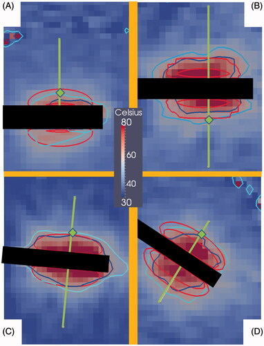
The trivariate joint uncertainty of the absorption, scattering and anisotropy are input into the gPC simulations and compared to MRTI data acquired during four canine MRgLITT experiments. The comparison is provided in Figures 4–6. MRTI from the four canine MRgLITT procedures is shown in Figure 6. Contours of the 60 °C isotherm of the MRTI are compared to the 95% confidence interval of the gPC predictions. Locations of spatial and temporal profiles used in Figures 4 and 5 are shown. An additional simulation varying perfusion only and using optics parameters from white matter is shown to compare the differences in input parameters from white matter to grey matter, Figure 5(A). The white matter-based, ω-univariate simulation shown in Figure 5(A) is clearly much colder and led to the decision to use grey matter weighted optics parameters in the trivariate simulations, shown in Table I. Spatial and temporal profiles, seen in Figures 4 and 5, show that canines 1 and 2 had a majority of overlapping regions between the MRTI and the simulations’ 95% confidence intervals. It should be noted that canines 3 and 4’s disagreement occurs relatively distant from the laser fibre.

Figure 5. Plots A through D correspond to canines 1 through 4 at the same time points described in Figure 6. A also contains a perfusion univariate model that uses optical scattering and absorption from white matter tissue (violet). The black rectangles obfuscate the portions of the linear profiles that are on the laser fibres because those regions provide invalid comparisons. A suggests that white matter optical scattering and absorption parameters produce profoundly colder temperatures. In plots A and B the trivariate model tends to overlap the MRTI well. Plots C and D show some agreement near the fibre (±∼3 mm), but diverge at further distances.

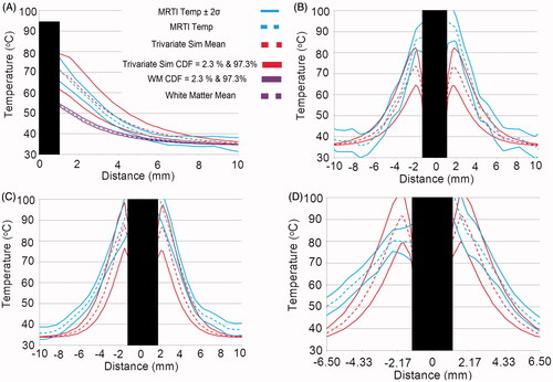
Figure 6. These images are MRTI from the four canine normal brain MRgLITT ablations. All images are from a slice that intersects the longitudinal axis of the laser applicator. Images A, B, C and D respectively correspond to canines 1, 2, 3 and 4 near maximum heating times t = 432 s, 222 s, 120 s, and 135 s. The superimposed green lines represent where the linear profiles for the four canines are plotted for Figures 4 and 5. Green diamonds indicate the location of temporal profiles in canine Figure 5. The black rectangles in each image are where the laser fibres were. The concentric red contours correspond to the predicted 60 °C isotherm contours with probabilities CDF = 2.3% and 97.7%. The areas between the red contours represent the central 95% of the model’s temperature distribution. According to the model, the CDF = 2.3% contour has a high probability of occurring, i.e. 97.7%. The dark blue and light blue contours respectively are the 60 °C isotherms from the MRTI temperature ±2σ of MRTI noise.

Discussion

A generalised polynomial chaos (gPC) method was used to propagate the uncertainty in the biothermal and optical parameters. A finite element-based stochastic form of the 3D Pennes bioheat transfer model was implemented for these purposes. The ability to accept plausible distributions of the biothermal and optical parameters and output realistic distributions of the temperature mean and variance is a novel aspect of gPC-based simulation. In a probabilistic bioheat simulation the challenge shifts from utilising the most precise constitutive values to identifying an appropriate input distribution. However, when using gPC, the model input distributions are limited to the Wiener–Askey scheme [39]. The two distributions considered were the Gaussian and uniform distributions. Because Gaussian distributions have been successfully and ubiquitously applied to probabilistic natural phenomena, Gaussian distributions were initially identified as an option. However, Gaussian distributions are positive from −∞ to +∞. In order to be physical, the constitutive values must be positive. If a Gaussian distribution was applied to the constitutive input distributions, the model would be influenced by non-physical inputs. The uniform distribution was chosen for use in the constitutive value distributions because it is straightforward to restrict the distribution to physical values.

The sensitivity study, displayed in Figure 2, shows the output variance of the five univariate models. It is important to note the relative input variance, based on published literature values, to the output variance. For example, ω is varied from 3 to 9 kg m⁻³s⁻¹, i.e. the variance is the mean ±50%. When compared to the variance of μ_a (mean ± 20%), it is evident that the BHTE is much more sensitive to μ_a than ω. Namely, even though ω is proportionally varied more than μ_a, the output temperature variance due to ω is considerably less than μ_a. The parameters found to produce the greatest variances were the optical parameters. Further, for the parameter range considered, the confidence intervals of temperature simulations using non-linear temperature and damage-dependent perfusion, scattering, and absorption (Equation 3) is bounded by the linear temperature simulations. Within this statistical setting, the linear problem with its associated uncertainty is used as a surrogate for the more complex non-linear bioheat transfer phenomena. The linear form of the optical parameters, μ_a, μ_s, and g, were used in the trivariate gPC-based MRgLITT simulations for comparison with the phantom experiments and canine ablations.

Comparison of worst-case scenarios and gPC estimates, Figure 2(D), demonstrate that the deterministic worst-case scenarios do not adequately capture the bulk of the statistical information in multivariate simulations, the worst-case scenarios only indicate the extrema. This is particularly true as the joint uncertainty of progressively more parameters is expanded in probability space. It is conceivable that worst-case scenarios could approximate gPC estimates in special cases, for example univariate simulations or parameters with low sensitivity yielding low output variance. However, these same special cases are less likely to require uncertainty quantification, which is the reason we used to legitimise our focus on the optics when comparing the trivariate models for the gPC-based MRgLITT simulations.

A more exhaustive application of uncertainty quantification to LITT would also examine the effect of other bioheat parameters, for example ρ, c_t, and u_a, and thermal dose parameters. Uncertainty in the dose parameters (either Arrhenius or cumulative effective minute (CEM) models) [70] depends on the temporal length of the hyperthermia treatment. In the case of relatively temporally short, spatially small >60 °C ablations, thermal dose models predict the spatial transition between coagulative necrosis of tissue and survival is small. However, for sub-ablative hyperthermia where thermal dose is accumulated over greater time, variance in thermal dose parameters may lead to appreciable spatial variance in the lethal threshold region or other interesting thermal dose levels. Future studies should investigate uncertainty in thermal dose parameters’ effect on thermal dose uncertainty, especially for temporally longer hyperthermia treatments.

Regarding the MRTI for canine 1, Figures 4–6, it should be noted that the canine’s brain ventricle was punctured by the catheter. The ventricle leaked cerebral spinal fluid (CSF) into the catheter’s insertion tract and ultimately pooled near one side of the laser fibre. The effect of the CSF on the thermal ablation can be seen as reduced temperature for the lower side of the thermal lesion in Figure 1. The effect is most obvious in the MRTI’s 60 °C isotherms. The model did not account for the presence of the CSF and therefore the regions affected by the CSF were excluded from analysis. Regarding the MRTI in general, the pixels imaging the laser fibre and very proximal regions affected by susceptibility artefact were not included in the linear profiles or isotherm contours. Further sources of discrepancy between simulation and MRTI during the cooling regime, Figures 3(C) and 4, are not seen in studies with external optical fibres [71] and are likely due to inaccuracies of the Dirichlet boundary condition to model the convective cooling of the catheter. Validation of physics-based models [72,73] of the convective heat transfer of the cooling fluid through the laser applicator is a topic of future work.

Despite multivariate gPC expansions being more appropriate for thermal therapy simulation, univariate gPC expansions may be used in future investigations to identify which parameters create the greatest variance of the temperature output, and subsequently restrict the gPC expansion to parameters that affect the temperature output the greatest. Improving the input distributions for the constitutive values should be investigated. Ideally, the model’s constitutive distributions would reflect the natural distributions of the constitutive parameters. The Wiener–Askey scheme includes gamma and beta distributions that are each a set of parameterised distributions. Both gamma and beta distributions include distributions that are not negative and resemble the Gaussian distribution’s distinctive ‘bell curve’. While Gaussian-like distributions exist, there is presently no particular reason any single distribution should work best. It may be sufficient to attempt an array of distributions in order to discover distributions that minimise the difference between the model and MRTI. Future investigations should additionally explore further statistical metrics of the model’s outcome. Possible tests include using spatio-temporal pixel-wise statistical tests for the difference or similarity between the model’s mean and MRTI’s temperature. The common example test for the difference of means is the Student’s t-test, however, the model’s polynomial expansion is not generally a Gaussian distribution so other tests should be sought.

This investigation took the natural step of comparing the model’s confidence interval to the MRTI’s confidence interval. In the case of gPC, the polynomial expansion probability distribution function was integrated to yield the polynomial expansion’s CDF. The CDF in turn indicated the probability of a threshold temperature (e.g. the temperature is >60 °C) as a function of distance from the laser fibre. These probabilities have a clear use in planning for thermal ablations. A stochastic simulation with temperature UQ gives the surgeon a probabilistic measure of the temperature. There are at least two methods of clinically using temperature UQ. First, the physician can plan the ablation using the stochastic model’s mean temperature prediction and the variance about the mean. For example, if a physician observes a large variance about the mean, the simulation cannot be implicitly trusted. Alternatively, temperature UQ could aid ablation planning by displaying an isotherm that is very likely to occur. For example, the physician could plan the ablation based on the CDF = 5% level. That is, the model would display a treated region that has a 95% chance of occurring. While deterministic thermal predictions do not have a measure of their uncertainty, a stochastic simulation provides confidence intervals. An example would be a surface contour that demarcates a volume that has at least a 95% probability of reaching 60 °C. Uncertainty quantification to create a ‘high probability of treatment’ contour is a highly desired goal. An accurate, high probability of treatment contour would allow physicians to quantify a measure of the probability of success. Also, there is little risk of overtreatment if the contour exceeds the desired treatment region; MRgLITT’s real-time MRTI provides the physician with feedback for ceasing treatment.

In conclusion, results demonstrate the utility of generalised polynomial chaos (gPC) expansion techniques to propagate parameter uncertainties through the computer model of bioheat transfer, and quantify uncertainties in the resulting output temperature distributions. Given parameter uncertainties and mathematical modelling approximations of the Pennes bioheat model, the 95% confidence intervals within the statistical framework demonstrate conservative estimates of the thermal therapy outcome and have potential for use as a computational prediction tool for thermal treatment planning.

Declaration of interest

The research in this paper was supported in part through NIH grants 5T32CA119930-03, 1R21EB010196-01, CA016672, and TL1TR000369. Canine data was obtained from BioTex, under grants R43-CA79282, R44-CA79282, R43-AG19276. The authors would also like to thank the DAKOTA [67], ITK [74], Paraview [75], PETSc [18], libMesh [76], and CUBIT [66] communities for providing enabling software for scientific computation and visualisation. Simulations were performed using allocations at the Texas Advanced Computing Center. The authors alone are responsible for the content and writing of the paper.

Acknowledgements

The authors are grateful for discussions with Ivo Babuška on uncertainty quantification applied to non-linear partial differential equations.

References

- Carpentier A, Itzcovitz J, Payen D, George B, McNichols RJ, Gowda A, et al. Real-time magnetic resonance-guided laser thermal therapy for focal metastatic brain tumors. Neurosurgery 2008;63:ONS21–9
- Rahmathulla G, Recinos PF, Valerio JE, Chao S, Barnett GH. Laser interstitial thermal therapy for focal cerebral radiation necrosis: A case report and literature review. Stereotact Funct Neurosurg 2012;90:192–200
- Carpentier A, McNichols RJ, Stafford RJ, Guichard J-P, Reizine D, Delaloge S, et al. Laser thermal therapy: Real-time MRI-guided and computer-controlled procedures for metastatic brain tumors. Lasers Surg Med 2011;43:943–50
- Carpentier A, Chauvet D, Reina V, Beccaria K, Leclerq D, McNichols RJ, et al. MR-guided LITT for recurrent glioblastomas. Lasers Surg Med 2012;44:361–8
- Jethwa PR, Barrese JC, Gowda A, Shetty A, Danish SF. Magnetic resonance thermometry-guided laser-induced thermal therapy for intracranial neoplasms: Initial experience. Neurosurgery 2012;71:133–45
- Curry DJ, Gowda A, McNichols RJ, Wilfong AA. MR-guided stereotactic laser ablation of epileptogenic foci in children. Epilepsy Behavior 2012;24:408–14
- Hawasli AH, Ray, WZ, Murphy RKJ, Dacey RG Jr, Leuthardt EC. Magnetic resonance imaging-guided focused laser interstitial thermal therapy for subinsular metastatic adenocarcinoma: Technical case report. Neurosurgery 2012;70:332–8
- McNichols RJ, Gowda A, Kangasniemi M, Bankson JA, Price RE, Hazle JD. MR thermometry-based feedback control of laser interstitial thermal therapy at 980 nm. Lasers Surg Med 2004;34:48–55
- Ulrich F. Interstitial laser irradiation of cerebral gliomas. Med Laser Appl 2005;20:119–24
- Fuentes D, Feng Y, Elliott A, Shetty A, McNichols RJ, Oden JT, et al. Adaptive real-time bioheat transfer models for computer-driven MR-guided laser induced thermal therapy. IEEE Trans Biomed Eng 2010;57:1024–30
- Woodrum DA, Gorny KR, Mynderse LA, Amrami KK, Felmlee JP, Bjarnason H, et al. Feasibility of 3.0 T magnetic resonance imaging-guided laser ablation of a cadaveric prostate. Urology 2010;75:1514. e1–6
- Fuentes D, Yung J, Hazle J, Weinberg J, Stafford R. Kalman filtered MR temperature imaging for laser induced thermal therapies. IEEE Trans Med Imaging 2011;31:984–94
- Roujol S, Denis de Senneville B, Hey S, Moonen C, Ries M. Robust adaptive extended Kalman filtering for real time MR-thermometry guided HIFU interventions. IEEE Trans Med Imaging 2012;31:533–42
- Potocki JK. Concurrent hyperthermia estimation schemes based on extended Kalman filtering and reduced-order modelling. Int J Hyperthermia 1993;9:849–65
- Todd N, Payne A, Parker DL. Model predictive filtering for improved temporal resolution in MRI temperature imaging. Magn Reson Med 2010;63:1269–79
- Mougenot C, Quesson B, De Senneville BD, De Oliveira PL, Sprinkhuizen S, Palussière J, et al. Three-dimensional spatial and temporal temperature control with MR thermometry-guided focused ultrasound (MRgHIFU). Magn Reson Med 2009;61:603–14
- Fuentes D, Oden JT, Diller KR, Hazle JD, Elliott A, Shetty A, et al. Computational modeling and real-time control of patient-specific laser treatment of cancer. Ann Biomed Eng 2009;37:763–82
- Minden V, Smith B, Knepley MG. Preliminary implementation of PETSc using GPUs. In: Yuen DA, Wang L, Chi X, Johnsson L, Ge W, Shi Y, eds. GPU solutions to multi-scale problems in science and engineering. Berlin: Springer; 2013. pp. 131--40
- Deisher M, Smelyanskiy M, Nickerson B, Lee VW, Chuvelev M, Dubey P. Designing and dynamically load balancing hybrid LU for multi/many-core. Comput Sci Res Dev 2011;26:211–20
- Chen CR, Miga MI, Galloway Jr RL. Optimizing electrode placement using finite-element models in radiofrequency ablation treatment planning. IEEE Trans Biomed Eng 2009;56:237–45
- Schwarzmaier HJ, Yaroslavsky IV, Yaroslavsky AN, Fiedler V, Ulrich F, Kahn T. Treatment planning for MRI-guided laser-induced interstitial thermotherapy of brain tumors: The role of blood perfusion. J Magn Reson Imaging 1998;8:121–7
- De Greef M, Kok HP, Correia D, Bel A, Crezee J. Optimization in hyperthermia treatment planning: The impact of tissue perfusion uncertainty. Med Phys 2010;37:4540–51
- Prakash P, Diederich CJ. Considerations for theoretical modelling of thermal ablation with catheter-based ultrasonic sources: Implications for treatment planning, monitoring and control. Int J Hyperthermia 2012;28:69–86
- Fuentes D, Cardan R, Stafford RJ, Yung J, Dodd GD, Feng Y. High-fidelity computer models for prospective treatment planning of radiofrequency ablation with in vitro experimental correlation. J Vasc Intervent Radiol 2010;21:1725–32
- Pennes HH. Analysis of tissue and arterial blood temperatures in the resting forearm. J Appl Physiol 1948;1:93–122
- Kim B-M, Jacques SL, Rastegar S, Thomsen S, Motamedi M. Nonlinear finite-element analysis of the role of dynamic changes in blood perfusion and optical properties in laser coagulation of tissue. IEEE J Select Topics Quantum Electron 1996;2:922–33
- Mohammed Y, Verhey JF. A finite element method model to simulate laser interstitial thermo therapy in anatomical inhomogeneous regions. Biomed Eng Online 2005;4:2
- Fuentes D, Walker C, Elliott A, Shetty A, Hazle JD, Stafford RJ. Magnetic resonance temperature imaging validation of a bioheat transfer model for laser-induced thermal therapy. Int J Hyperthermia 2011;27:453–64
- Xiu D. Numerical methods for stochastic computations: A spectral method approach. Princetion, NJ: Princeton University Press; 2010
- Dos Santos I, Haemmerich D, Schutt D, Da Rocha AF, Menezes LR. Probabilistic finite element analysis of radiofrequency liver ablation using the unscented transform. Physics in medicine and biology 2009;54(3):627–40
- Fahrenholtz S, Fuentes D, Stafford R, Hazle J. SU-F-BRCD-08: Uncertainty Quantification by Generalized Polynomial Chaos for MR-Guided Laser Induced Thermal Therapy. Proceeding at the 54th Annual Meeting for the American Association of Physicists in Medicine, Charlotte, NC. July 2012 [cited 29 Oct 2012]. pp. 3857–3857
- Niederreiter H. Quasi-Monte Carlo methods and pseudo-random numbers. Bull Am Math Soc 1978;84:957–1041
- McKay MD, Beckman RJ, Conover WJ. A Comparison of three methods for selecting values of input variables in the analysis of output from a computer code. Technometrics 1979;21:239–45
- Smith RL. Efficient Monte Carlo procedures for generating points uniformly distributed over bounded regions. Operations Res 1984;32:1296–308
- Prudencio E, Schulz K. The parallel C++ statistical library QUESO™: Quantification of uncertainty for estimation, simulation and optimization. In: Alexander M, D’Ambra P, Belloum A, Bosilca G, Cannataro M, Danelutto M, editors. Euro-Par 2011: Parallel processing workshops. Berlin: Springer, 2012. pp 398–407
- Prudencio E, Cheung SH. Parallel adaptive multilevel sampling algorithms for the Bayesian analysis of mathematical models. Int J Uncertain Quantification 2012;2:215–37
- Wiener N. The homogeneous chaos. Am J Math 1938;60:897–936
- Ghanem RG, Spanos PD. Stochastic finite elements: A spectral approach. New York: Springer; 1991
- Xiu D, Karniadakis GE. The Wiener–Askey polynomial chaos for stochastic differential equations. SIAM J Sci Comput 2002;24:619–64
- Xiu D, Karniadakis GE. Modeling uncertainty in steady state diffusion problems via generalized polynomial chaos. Comput Methods Appl Mech Eng 2002;191:4927–48
- Geneser SE, Hinkle JD, Kirby RM, Wang B, Salter B, Joshi S. Quantifying variability in radiation dose due to respiratory-induced tumor motion. Med Image Anal 2011;15:640–9
- Reagan MT, Najm HN, Ghanem RG, Knio OM. Uncertainty quantification in reacting-flow simulations through non-intrusive spectral projection. Combust Flame 2003;132:545–55
- Cassell JS, Williams MMR. An approximate method for solving radiation and neutron transport problems in spatially stochastic media. Ann Nucl Energy 2008;35:790–803
- Kewlani G, Iagnemma K. A multi-element generalized polynomial chaos approach to analysis of mobile robot dynamics under uncertainty. IEEE Proceedings of the International Conference on Intelligent Robots and Systems, 2009, pp. 1177–1182
- Oden T, Moser R, Ghattas O. Computer predictions with quantified uncertainty, Part I. SIAM News 2010;43:1–3
- Yaroslavsky AN, Schulze PC, Yaroslavsky I V, Schober R, Ulrich F, Schwarzmaier HJ. Optical properties of selected native and coagulated human brain tissues in vitro in the visible and near infrared spectral range. Phys Med Biol 2002;47:2059–73
- Kreith F. The CRC handbook of thermal engineering. Berlin: Springer; 2000
- Huttunen JMJ, Huttunen T, Malinen M, Kaipio JP. Determination of heterogeneous thermal parameters using ultrasound induced heating and MR thermal mapping. Phys Med Biol 2006;51:1011–32
- Yung JP, Shetty A, Elliott A, Weinberg JS, McNichols RJ, Gowda A, et al. Quantitative comparison of thermal dose models in normal canine brain. Med Phys 2010;37:5313–21
- Valvano JW. Tissue thermal properties and perfusion. In: Welch AJ, Gemert MJC, editors. Optical-thermal response of laser-irradiated tissue. Berlin: Springer; 2011. pp 455–85
- Madsen SJ, Wilson BC. Optical properties of brain tissue. In: Madsen SJ, editor. Optical methods and instrumentation in brain imaging and therapy. New York: Springer; 2013. pp 1–22
- Beek JF, Blokland P, Posthumus P, Aalders M, Pickering JW, Sterenborg HJCM, et al. In vitro double-integrating-sphere optical properties of tissues between 630 and 1064 nm. Phys Med Biol 1997;42:2255–61
- Valvano JW, Cochran JR, Diller KR. Thermal conductivity and diffusivity of biomaterials measured with self-heated thermistors. Int J Thermophys 1985;6:301–11
- Diller KR, Valvano JW, Pearce JA. Bioheat transfer. In: Kreith F, editor. The CRC handbook of thermal engineering. Boca Raton, FL: CRC Press; 2000. pp 4–114 to 4–215
- Duck FA. Physical properties of tissue: A comprehensive reference book. London: Academic Press; 1990
- Dewhirst MW, Viglianti BL, Lora-Michiels M, Hanson M, Hoopes PJ. Basic principles of thermal dosimetry and thermal thresholds for tissue damage from hyperthermia. Int J Hyperthermia 2003;19:267–94
- Henriques FC, Moritz AR. Studies of thermal injury: I. The conduction of heat to and through skin and the temperatures attained therein. A theoretical and an experimental investigation. Am J Pathol 1947;23:530–49
- Pickering JW, Prahl SA, Van Wieringen N, Beek JF, Sterenborg HJ, Van Gemert MJ. Double-integrating-sphere system for measuring the optical properties of tissue. Appl Optics 1993;32:399–410
- Yaroslavsky I, Yaroslavsky A. Inverse hybrid technique for determining the optical properties of turbid media from integrating-sphere measurements. Appl Optics 1996;35:6797–809
- Germer CT, Roggan A, Ritz JP, Isbert C, Albrecht D, Müller G, et al. Optical properties of native and coagulated human liver tissue and liver metastases in the near infrared range. Lasers Surg Med 1998;23:194–203
- Schwarzmaier H, Yaroslavskya A, Yaroslavsk I, Goldbacha T, Kahn T, Ulrichc F, et al. Optical properties of native and coagulated human brain structures. Proc. SPIE 2970, Lasers in Surgery: Advanced Characterization, Therapeutics, and Systems VII, 492 (22 May 1997); doi:10.1117/12.275082
- Ritz JP, Roggan A, Germer CT, Isbert C, Müller G, Buhr HJ. Continuous changes in the optical properties of liver tissue during laser-induced interstitial thermotherapy. Lasers Surg Med 2001;28:307–12
- Friebel M, Do K, Hahn A, Mu G, Berlin D, Medizin L, et al. Optical properties of circulating human blood in the wavelength range 400–2500 nm. J Biomed Optics 1999;4:36–46
- Bankson JA, Stafford RJ, Hazle JD. Partially parallel imaging with phase-sensitive data: Increased temporal resolution for magnetic resonance temperature imaging. Magn Reson Med 2005;53:658–65
- Dickey DJ, Partridge K, Moore RB, Tulip J. Light dosimetry for multiple cylindrical diffusing sources for use in photodynamic therapy. Phys Med Biol 2004;49:3197–208
- Blacker TD, Bohnhoff WJ, Edwards T. CUBIT mesh generation environment. Vol. 1: Users manual. Albuquerque, NM: Sandia National Laboratories; 2004
- Eldred MS, Giunta AA, Van Bloemen Waanders BG, Wojtkiewicz SF, Hart WE, Alleva MP. DAKOTA, a multilevel parallel object-oriented framework for design optimization, parameter estimation, uncertainty quantification, and sensitivity analysis: Version 4.1 reference manual. Albuquerque, NM: Sandia National Laboratories; 2007
- Butler T, Dawson C, Wildey T. A posteriori error analysis of stochastic differential equations using polynomial chaos expansions. SIAM J Sci Comput 2011;33:1267–91
- Babuška I, Nobile F, Tempone R. Worst case scenario analysis for elliptic problems with uncertainty. Numerische Mathematik 2005;101:185–219
- Yarmolenko PS, Moon EJ, Landon C, Manzoor A, Hochman DW, Viglianti BL, et al. Thresholds for thermal damage to normal tissues: An update. Int J Hyperthermia 2011;27:320–43
- MacLellan C, Fuentes D, Schwartz J, Elliott A, Hazle J, Stafford RJ. Estimating nanoparticle optical properties with magnetic resonance temperature imaging and bioheat transfer simulation. Med Phys 2013;in press
- Fasano A, Hömberg D, Naumov D. On a mathematical model for laser-induced thermotherapy. Appl Math Model 2010;34:3831–40
- Feng Y, Fuentes D. Model-based planning and real-time predictive control for laser-induced thermal therapy. Int J Hyperthermia 2011;27:751–61
- Ibanez L, Schroeder W, Ng L, Cates J. The ITK software guide, 2nd ed. Clifton Park, NY: Kitware; 2005. Available from: http://www.itk.org/ItkSoftwareGuide.pdf
- Henderson A, Ahrens J. The ParaView guide: A parallel visualization application. Clifton Park, NY: Kitware; 2004
- Kirk BS, Peterson JW, Stogner RH Carey GF. libMesh – A C++ finite element library. CFDLab; 2003. Available from: http://libmesh.sourceforge.net
- Welch AJ, Gemert MJC, editors. Optical-thermal response of laser-irradiated tissue, 2nd ed. Berlin: Springer; 2011. p 951
- Cooper TE, Trezek GJ. Correlation of thermal properties of some human tissue with water content. Aerospace Med 1971;42:24–7
- Kapin MA, Ferguson JL. Hemodynamic and regional circulatory alterations in dog during anaphylactic challenge. Am J Physiology: Heart Circ Physiol 1985;249:H430–7
- Atzler E, Richter F. Über die Wärmekapazität des arteriellen und venösen Blutes. [About the heat capacity of arterial and venous blood] Beitr Chem Phys Pathol 1920;112:310–12