Numerical assessment of a criterion for the optimal choice of the operative conditions in magnetic nanoparticle hyperthermia on a realistic model of the human head

Abstract

Purpose: This paper presents a numerical study aiming at assessing the effectiveness of a recently proposed optimisation criterion for determining the optimal operative conditions in magnetic nanoparticle hyperthermia applied to the clinically relevant case of brain tumours.

Materials and methods: The study is carried out using the Zubal numerical phantom, and performing electromagnetic–thermal co-simulations. The Pennes model is used for thermal balance; the dissipation models for the magnetic nanoparticles are those available in the literature. The results concerning the optimal therapeutic concentration of nanoparticles, obtained through the analysis, are validated using experimental data on the specific absorption rate of iron oxide nanoparticles, available in the literature.

Results: The numerical estimates obtained by applying the criterion to the treatment of brain tumours shows that the acceptable values for the product between the magnetic field amplitude and frequency may be two to four times larger than the safety threshold of 4.85 × 10⁸A/m/s usually considered. This would allow the reduction of the dosage of nanoparticles required for an effective treatment. In particular, depending on the tumour depth, concentrations of nanoparticles smaller than 10 mg/mL of tumour may be sufficient for heating tumours smaller than 10 mm above 42 °C. Moreover, the study of the clinical scalability shows that, whatever the tumour position, lesions larger than 15 mm may be successfully treated with concentrations lower than 10 mg/mL. The criterion also allows the prediction of the temperature rise in healthy tissue, thus assuring safe treatment.

Conclusions: The criterion can represent a helpful tool for planning and optimising an effective hyperthermia treatment.

Keywords:

• Bioheat transfer equation
• electromagnetic fields
• Magnetic nanoparticles hyperthermia
• optimisation criterion
• Zubal numerical phantom

Introduction

Magnetic nanoparticle Hyperthermia (MNPH) [1–3] is a relatively new subclass of hyperthermia for cancer treatment, wherein the therapeutic heating of the tumour is achieved through the local infusion of magnetic nanoparticles (MNPs) and the application of a radio-frequency (RF) magnetic field (MF). MNPH is very promising for its therapeutic efficacy and the minimal side effects, as proven by an increasing number of clinical studies carried out on patients suffering from different types of cancer [4–11]. These peculiarities are essentially due to the capability of achieving a highly localised heating of the tumour thanks to the possibility of selectively accumulating the MNPs in the tumour, to their remarkable magnetic losses in the RF range, and to the very weak magnetic response and high transparency of human tissues to RFMF [12]. Indeed, while the first two features allow the achievement of a significant and localised heating of the tumour, the third feature enables the achievement of such heating producing only a secondary heating in the remaining exposed tissue (even if this region is much larger than the tumour), due to induced eddy currents.

MNPH is also appealing because of the possibility of treating deep tumours in the body such as prostate [3–5], brain [6–9] and bone cancers [10] (again, thanks to the high transparency of the human body to RFMF), barely treatable with other kinds of hyperthermia (such as ultrasound, microwave or laser hyperthermia), and for the minimal invasiveness of the MNP administration techniques, namely by direct injection [9] into the tumour or in a systemic way using passive and/or active biochemical targeting [13].

From a clinical standpoint, one of the main challenges in MNPH is to achieve therapeutic heating of the tumour with a dosage of MNPs as small as possible. Minimising the dosage of MNPs is desirable not only for minimising possible side effects and facilitating their elimination, but also to make possible the delivery of MNPs intravenously, via passive and/or active targeting, which, while being more selective and efficient than direct injection into the tumour, allows delivery of smaller amounts of MNPs. This goal can be fruitfully reached by properly setting the amplitude and frequency of the applied MF, as well as the MNP size. However, this is not a trivial task because at the same time one has to limit the heating of the exposed healthy tissue due to the induced eddy currents, which, while being a second-order effect as compared to the heating produced by the MNPs in the tumour, involves a much larger region, and so could lead to severe overheating of healthy tissues.

An effective optimisation criterion has been recently presented [14]. The criterion is very simple and involves two steps: in the first, by means of a thermal analysis we determine the optimal levels of the magnetic and electric power densities to be dissipated in the tumour and in the normal tissue for heating up the tumour above a therapeutic temperature, while keeping all the healthy tissues, outside a (small) transition region, below a safety temperature. Once these power levels were determined, the optimal MF and MNP parameters, and the corresponding minimum dosage of MNPs, were estimated by using the models describing the various energy dissipation mechanisms responsible for the heating in MNPH, which relate all these quantities together.

In our previous works [14,15], only a simplified numerical study was carried out, involving electrically and thermally homogeneous tissues and/or canonical geometries, which just aimed at giving a preliminary proof of the usefulness of the criterion. These preliminary results provided useful indications on the allowable values for the MF amplitude and frequency, on the minimum MNP dosage, on the clinical scalability of MNPH and on the levels of heating reached in the tissues during the treatment. In particular, except for poorly perfused tissues, the values of the fundamental parameter, given by the product of the MF amplitude by the frequency, were significantly larger than the empirical threshold of 4.85 × 10⁸ A/m/s, usually adopted in order to assure treatment safety. Consequently, the required MNP concentrations were smaller than those typically quoted in the literature for treating tumours of comparable sizes, thus suggesting that the application of the criterion may significantly improve the MNPH performances.

The aim of this paper is to numerically validate the criterion in Bellizzi et al. [14,15] in the more challenging and clinically relevant case of brain tumours, by using a 3D realistic model of the human body. To this end, an exhaustive numerical analysis was carried out, by employing as a model the well-known anthropomorphic Zubal numerical phantom available in the literature [16]. The input data for the proposed criterion were generated by performing electromagnetic-thermal co-simulations with the aid of a commercially available multi-physics software, the CST Studio Suite (Darmstadt, Germany). Brain tumours of different sizes and positions were considered.

The results concerning the optimal therapeutic concentration of MNPs obtained through the analysis are validated using experimental data on the specific absorption rate of iron oxide nanoparticles.

Finally, by using the criterion, the limits of the clinical scalability of the MNPH for the treatment of brain tumours in adult patients were estimated.

The paper is organised as follows. An overview of the optimisation criterion is given in the second section. The detailed descriptions of the numerical phantom employed and of the simulation set up are provided in the third section, whereas the main results of the numerical analysis are presented in the fourth section. Conclusions follow.

Overview of the optimisation criterion

The goal of the optimisation is to search those values of MF amplitude, say H (H is the amplitude of MF within the tumour, which can be safely assumed uniform, thanks to the relatively small tumour size as compared to the spatial variability of the MF), working frequency, say f, and MNPs size, say d, that minimise the mean concentration of MNPs in the tumour, say c, (usually the MNP distribution in the tumour following direct injection is not uniform; therefore, we define a mean MNP concentration given by the ratio between total amount of injected MNPs and the tumour volume), required for heating up the tumour above a therapeutic temperature, say T₁, while keeping the surrounding healthy tissue, outside a given transition region, below a safety temperature, say T₂. To this respect, the first step is to relate c to H, f, d and to the temperature rise produced over the exposed tissues by the treatment. This can be done by using the models describing the energy dissipation mechanisms responsible for the heating in MNPH.

Concerning MNP losses, for an ensemble of mono-dispersed MNPs suspended in a viscous environment, two different kinds of mechanisms of losses can arise in an alternating MF: relaxation losses or hysteresis losses. Therefore, two different models were adopted. If the MNPs are ultrafine (core size smaller than 10 nm for iron oxide MNP) or single grain superparamagnetic particles (this can be confidently assumed at least up to a core size of 20 nm for iron oxide MNP [17]), then relaxation is the dominant loss mechanism and the following expression can be used for the mean magnetic power density dissipated by the MNPs in the tumour [18]: (1)

In Equation 1(1) , H, f, d and c (expressed in mg of MNPs/mL of tumour) were defined above, ρ is the mass density of the material of the MNP core, μ₀ the permeability of the vacuum, M_d the domain magnetisation of each MNP, L(ξ) the Langevin function, k_B the Boltzmann constant, T the temperature (in °Kelvin), k_a the anisotropy constant of the MNPs and τ₀ a characteristic time depending on the composition of the MNP core. (While in Bellizzi et al. [14,15] a quadratic dependence on H was assumed for p_h given by Equation 1(1) , here the dependence is non-quadratic, due to the presence of L(ξ), which takes into account the saturation of the magnetisation of the MNPs when exposed to a high MF. The main consequence of this is an increase in the required amount of MNPs to be infused for achieving the therapeutic heating of the tumour). The more realistic case of poly-dispersed MNPs (i.e. MNPs characterised by a core size distribution) can be dealt with by averaging Equation 1(1) over the core size distribution. It is worth noting that with reference to the averaged version of Equation 1(1) , there are several works available in the literature [19–24] showing a substantial agreement between the experimental SAR and the theoretical forecasts, provided that one correctly sets the values of the physical parameters involved in Equation 1(1) , which depend on several variables such as size, shape, crystal lattice, coating, for example. These values can be obtained by fitting the data from an exhaustive measurement campaign.

Alternatively, if the MNPs are multi-domain or single domain, but multi-grain and closely packed particles, then hysteresis losses are the dominant dissipation mechanism and the following model, experimentally verified in Hergt et al. [25], can be used: (2) where the coercivity, H_c(d), is given by Equation 3(3) . (3)

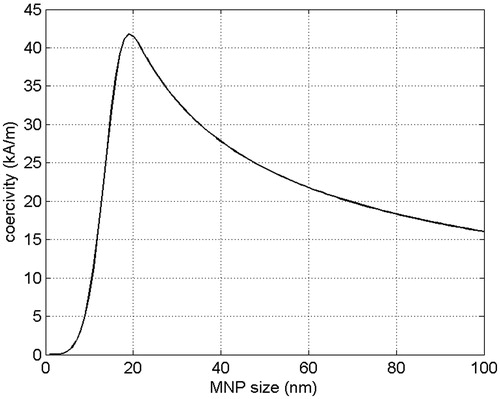
The typical behaviour of H_c(d) for an ensemble of MNPs is shown in Figure 1. In Equations 2(2) and 3(3) M_r is the remanent magnetisation of the ensemble of MNPs, while α, H_M and d₁ are fitting parameters whose values depend on the MNP type [25]. Also in this case, with reference to the averaged version of Equations 2(2) and 3(3) , there are several works available in the literature [17,24–26] showing a substantial agreement between the experimental SAR and the theoretical forecasts, provided that, as already stressed, the values of the physical parameters involved in Equations 2(2) and 3(3) , are properly set.

Figure 1. Coercivity versus MNP size for an ensemble of magnetite nanoparticles.

Concerning this last point, it is worth noting that once in biological medium, the MNPs, especially those having a large core, may aggregate and form large clusters, which, because of the strong interactions among the dipoles of each MNP, may exhibit a SAR significantly different from that of non-agglomerated MNPs [27,28]. Accordingly, in determining the values of the parameters involved (and even before, in determining the model of energy dissipation to be adopted), by fitting experimental data, it is convenient to carry out the experiments under conditions which are as close as possible to those of clinical application. To this end, measurement techniques allowing the characterisation of the response of diluted suspension of MNP in biological media should be adopted [29].

The other loss mechanism is the electric power dissipation, via the Joule effect, due to the induced eddy currents, which is clearly given by the Joule law. More specifically, as long as inductive applicators and sufficiently low frequencies are used, as happens in MNPH, a linear relationship can be assumed between the induced electric field (EF) amplitude, say E(r), and the product Hf, namely: E(r) = Hfe(r), where the function e(r) takes into account the spatial variability of the EF (r is the position vector in a fixed reference frame). As a result, the mean value over the whole exposed tissue, Ω, of such electric power density is given by Equation 4(4) . (4) where σ(r) is the electric conductivity of the tissues (the dependence on r takes into account the electric inhomogeneity of the human tissues) and z = < 1/2σ  (r) e (r)² >_Ω, < >_Ω denoting the spatial average over Ω. It is worth noting that, in principle, z depends on f, due to the frequency dispersion of the electric properties of the human tissues [30]. However, as will be shown by the numerical results reported in the fourth section, this dependence can be ignored over the frequency band of 50–200 kHz considered, which is typically the range of interest in MNPH.

By combining Equation 4(4) with one of Equation 1(1) , or 2(2) one gets the searched expression for c, i.e. for the objective function to be minimised. For instance, by using Equation 1(1) one gets the following expression for c in terms of the unknown parameters p_h, p_e, H, f and d: (5)

(the dependence on H is included in the Langevin parameter, ξ). Again, the more realistic case of poly-dispersed MNPs can be taken into account by averaging c over the MNP size distribution. In this case, the unknown d represents the mean value of such size distribution. Similar dependence, for brevity not reported, is obtained by using Equation 2(2) in place of Equation 1(1) [14].

Accordingly, the optimal values of p_h, p_e, H, f and d are determined as Equation 6(6) : (6) subjected to the temperature constraints (6a) (6b)

Ω₁ being the tumour region and Ω₂ a transition region containing the tumour, whose size represents the required degrees of spatial selectivity of the heating. Condition 6a reflects the requirement that all of the tumour must be heated above the therapeutic temperature T₁; condition 6b reflects the requirement that outside the transition region the healthy tissue must be kept below the safety temperature T₂, which is obviously lower than T₁. It is worth noting that the dependence of c on the temperature T is implicitly taken into account in p_h and p_e. Therefore, the imposed temperature constraints translate into constraints on p_h and p_e. Moreover, since c is the product of a function of only p_h and p_e by a function of only H, f and d (this is true by using either Equation 1(1) or 2(2) to derive c [14]), the searched p_hopt, p_eopt and H_opt, f_opt, d_opt can be obviously found separately in two steps: optimal choice of p_h and p_e and optimal choice of H, f and d. In the next subsections we will present a short overview of these two steps, by referring the reader to Bellizzi et al. [14] for a more comprehensive presentation.

Optimal choice of p_h and p_e

To estimate the optimal values of p_h and p_e the first step is to relate them to the temperature rise, T_Δ = T−T₀, produced over the exposed tissue, T₀ being the normal temperature of the human body (T₀ ≈ 37 °C). To this respect the steady-state the Pennes bioheat equation (PBHE) [31] can be employed. We use the steady state PBHE since in mild hyperthermia the therapeutic temperature rise in the tumour must be kept for at least 1 h in order to reach the therapeutic goal, a time long enough to allow the exposed region to reach the thermal equilibrium.

Blood perfusion as well as tissue thermal parameters involved in the PBHE depend on T, so that the PBHE is not linear. However, as will be shown in the following, the optimal operative conditions in MNPH must be determined by requiring that during the treatment the temperature does not exceed a safety temperature of 39 °C (i.e. T₂ = 39 °C in Equation 6b(6b) ) in all the exposed tissues, apart from a small transition region surrounding the tumour and the tumour itself, wherein the temperature must be larger than 42 °C to achieve the therapeutic goal (mild hyperthermia).

As already discussed in [14] (and in the references therein reported), below 39 °C the blood perfusion of the normal tissues only changes marginally with respect to the basal value. The same holds for the thermal properties, which for a temperature variation of at most 2 °C (with respect to the basal temperature T₀ ≈ 37 °C) can in practice be assumed constant. Therefore, the imposed thermal constraint 6b allows the adoption of a linear thermal model outside the transition region.

This is no longer true in the tumour (and possibly in the transition region), as an abrupt change of blood perfusion takes place at a temperature of about 42–43 °C. Notably, the blood perfusion of the healthy tissue rapidly grows, while that of several kinds of tumour even drops [32]. Therefore, because the temperature exceeds 42–43 °C only in the tumour, as the condition 6a requires, the adoption of a linear PBHE is expected to lead to an underestimation of the temperature inside the tumour, which is a conservative result from the clinical point of view.

Of course, the above conclusions hold as long as the heating in the healthy tissue is kept below certain levels (39 °C in our study). However, this is an essential safety constraint, as important as that of achieving the therapeutic heating of the tumour, in order to preserve the healthy tissue from the side effects due to a long and excessive overheating. This is particularly true in the case we are considering, namely that of brain tumours.

Moreover, given the relatively small temperature ranges of our interest, it is doubtful that taking into account the temperature dependence of the thermal parameters (or adopting a more sophisticated thermal model) would lead to more reliable results, due to the unavoidable incertitude in the values of such parameters.

Once the temperature dependence of the thermal properties of the tissues is neglected, the PBHE becomes linear, so that T_Δ can be expressed as follows. (7)

The four terms on the right side of Equation 7(7) are the temperature increments produced respectively by the magnetic losses, say q_h(r), dissipated by the MNPs in the tumour (p_h = <q_h(r)>_Ω1), the electric losses, say q_e(r), dissipated via Joule effect by the induced eddy currents (p_e = <q_e (r)>_Ω), the metabolic heat generation rate, say q_m(r) (p_m = <q_m(r)>_Ω), the thermal exchange with the external environment, at a temperature T = T_ext. Consequently, T_Δh(r), T_Δe(r), T_Δm(r) and T_Δext(r) are the increments for unitary values of p_h, p_e, p_m and T_ext − T₀, respectively, namely the solutions of the steady-state PBHE respectively for: (p_h, p_e, p_m) = (1,0,0) W/m³ and T_ext − T₀ = 0 °C; (p_h, p_e, p_m) = (0,1,0) W/m³ and T_ext − T₀ = 0 °C; (p_h, p_e, p_m) = (0,0,1) W/m³ and T_ext − T₀ = 0 °C; (p_h, p_e, p_m) = (0,0,0) W/m³ and T_ext − T₀ = 1 °C. These increments can be numerically evaluated by carrying out electromagnetic and thermal simulations (the electromagnetic simulations are required for evaluating q_h(r) and q_e(r), which in turn are required for computing T_Δh(r) and T_Δe(r)), once an accurate model of the exposure system and an accurate (and specific patient) model of the region of the body to be exposed, from both electromagnetic and thermal points of view, are available. (A study of the sensitivity of each term in Equation 7(7) against the uncertainty in the knowledge of the thermal properties of the exposed tissues can be found in Bellizzi and Bucci [33].) From a practical standpoint, the latter can be built by using previously acquired MRI or CT images of the patient, as in the case of the Zubal numerical phantom [16]. Once these increments have been determined by imposing the temperature constraints 6a and 6b one has Equations 8 and 9: (8) (9) where ΔT₁₍₂₎ = T₁₍₂₎−T₀. As shown in [14], this is equivalent to require that (10) (11) where the quantities F_h and F_e are solutions of the system of equations obtained by replacing the inequalities with equalities into Equations 8(8) and 9(9) , whose expression can be found in Bellizzi et al. [14]. Equations 10(10) and 11(11) translate the temperature constraints 6a and 6b into constraints on p_h and p_e. Since c is proportional to the ratio p_h/p_e^1/2 (see Equation 5(5) and Bellizzi et al. [14]), p_hopt and p_eopt are obtained by choosing p_h as small as possible and p_e as large as possible, namely by setting the equality in both Equations 10(10) and 11(11) .

As a final remark, it is worth noting that the criterion is independent of the bioheat model adopted for evaluating T_Δh(r), T_Δe(r), T_Δm(r) and T_Δext(r), provided that linearity can be assumed.

Optimal choice of H, f and d

Since the dependence of c on H, f and d changes according to the adopted model for p_h, i.e. Equation 1(1) or 2(2) , we will distinguish between these two cases.

As shown in Bellizzi et al. [14], if Equation 1(1) is used for p_h, H_opt = H_max, H_max being the maximum MF amplitude that the exposure system can produce at the tumour position (H_max depends on exposure system, but also on the relative position of the tumour with respect to the system). Then, according to Equation 4(4) , f_opt = (p_eopt/z)^1/2/H_opt. Finally, d_opt is determined by requiring that 2πf_optτ_eff(d_opt) = 1.

On the other hand, if Equation 2(2) is used for p_h, H_opt ≈ 1.43H_cmax, where H_cmax is the maximum value of the coercivity, H_c(d), and d_opt is the MNP size at which H_c(d) reaches the maximum (see Figure 1). Again, f_opt = (p_eopt/z)^1/2/H_opt. It is worth noting that if H_max is smaller than 1.43H_cmax, the optimal choice for the MF amplitude is again H_opt = H_max. In this case d_opt is the solution of the equation 1.43Hc(d_opt) = H_max.

We would like stress that, as shown in Bellizzi et al. [14], all the above outlines stay valid in the more realistic case of poly-dispersed MNPs, characterised by a log-normal distribution for the size of the MNP core. Obviously, in this case d_opt is the mean value of such a size distribution. Later on, we will estimate H_opt, f_opt and d_opt and the corresponding minimum MNP concentration, say c_min, by using both Equations 1(1) and 2(2) for deriving the expression of c, properly averaged in order to take into account the MNP size distribution.

Numerical phantom and the simulation set-up

As already mentioned, the input data to the criterion, i.e. the increments T_Δh(r), T_Δe(r), T_Δm(r) and T_Δext(r) in Equation 7(7) , were generated by performing electromagnetic-thermal co-simulations with the aid of the CST Studio Suite software and using the Zubal numerical phantom. In the following we will provide the details of the numerical phantom, the simulation set-up and the adopted MNPs.

Numerical phantom

The Zubal numerical phantom consists of 87 × 147 × 493 cubic voxels of 3.6 mm in size and it was constructed by translating greyscale images from MRI and CT scans of an adult male patient (this procedure is the leading way to construct reliable numerical phantoms for treatment planning).

The original numerical phantom is provided as an array of 87 × 147 × 493 integers (from 0 to 125), where each integer identifies the type of tissue (e.g. brain, skin, bone) filling the voxel. Hence, the model to be used in the numerical simulations was constructed by assigning to each integer the electric and thermal properties of the corresponding tissue type, experimentally found in the literature [30,34]. A Cole–Cole model was adopted to take into account the frequency dispersion of the electric properties of the various tissues. In Table 1 we report some of the tissues composing the model together with the values of the thermal (the thermal conductivity, k, the blood perfusion rate, w_b, the specific heat capacity of blood, c_b, and the metabolic heat generation rate, q_m), and the electric properties (the relative permittivity, ɛ_r, and the electric conductivity, σ) at f = 50, 100, 200 kHz. The presence of the malignancy was simulated by including in the brain a spherical tumour having the same electric and thermal properties of the hosting tissue. Of course, the properties of brain tumours are expected to be different from those of normal brain, but, to the best of our knowledge, no experimental data are available. However, due to the relatively small size of the tumour assumed in our simulations, compared to the size of the whole irradiated region, these differences cannot significantly affect the final results. Thus, we can confidently neglect them.

Table 1. Thermal and electric properties of some human tissues in the band 50–200 kHz.

				ɛr			σ (S/m)
Tissue	k (W/m/°C)	cbwb (W/m^3/°C)	qm (W/m^3)	50 kHz	100 kHz	200 kHz	50 kHz	100 kHz	200 kHz
Skull	0.32	3400	610	264	228	204	0.02	0.021	0.021
CST	0.57	0	0	109	109	109	2	2	2
Grey matter	0.51	40000	7100	5461	3222	2010	0.13	0.13	0.14
Fat	0.20	1700	300	172	93	56	0.024	0.024	0.025
Muscle	0.49	2700	480	10094	8089	6378	0.35	0.36	0.38
Skin (dry)	0.37	9100	1620	1127	1119	1105	3 × 10^−4	4 × 10^−4	1 × 10^−3
White matter	0.48	40000	7100	3548	2108	1287	0.078	0.082	0.087

Tumours of different sizes and positions were considered, as summarised in Table 2. A view of the phantom, including the tumour positions, is shown in Figure 2(A).

Figure 2. A view of the model adopted in the simulation in CST software environment. (A) A cut of the numerical phantom, (B) exposure system and numerical phantom.

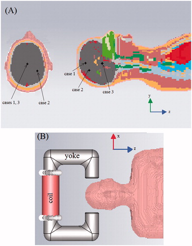
Table 2. Tumour and transition region positions and sizes considered in the numerical analysis.

	Tumour position
Case	x (cm)	y (cm)	z (cm)	Tumour size (mm)	Transition regionsize (mm)
1	−1.4	−3	−84	20	40
				15	30
2	2.1	−5	−82	20	40
				15	30
3	−1.4	−3	−78.5	20	40
				15	30

Simulation set-up

The temperature increments T_Δh(r) and T_Δe(r) were determined in two steps. In the first one, by means of an electromagnetic simulation, we determined the MF and the EF produced by the exposure system, from which we computed the normalised q_m(r) and q_e(r) dissipated in the tumour and in the surrounding healthy tissue, respectively. In the second step, these data were singularly processed by a thermal solver and the aforementioned temperature increments were determined. At this step, we also computed T_Δm(r) and T_Δext(r).

Concerning the electromagnetic simulation, we have considered an exposure system consisting of a U-shaped iron yoke with a coil of 1000 turns wound on it. The yoke has a circular section with a diameter of 8 cm and a spacing between the two poles (air-gap) of about 20 cm. A sketch of the system is shown in Figure 2(B). We want to stress that the design of the applicator goes beyond the aim of this work. Hence, a simple inductive applicator was chosen, disregarding any other requirement aiming at improving its performance and/or the MF uniformity. Since the system generates a non-uniform MF, the MF amplitude applied to the tumour depends on the tumour position in the air-gap. Hence, for each of the cases in Table 2, we moved the exposure system in such a way to put the tumour as much as possible at the air-gap centre, thereby simulating the behaviour of an optimised system. In this way, the MF applied to the tumour becomes independent of the tumour position and equal to that produced by the device at the air-gap centre.

The simulations were performed at different frequencies, in the band 50–200 kHz, by using a low frequency quasi-magneto-static solver, available in CST Studio Suite. An adaptive mesh refinement was set for the simulations, which stops when a relative error lower than 1% between the field energies in the exposed region, at two consecutive steps, is reached. Since the goal is the treatment of brain tumours, to save computational time only a portion of the Zubal numerical phantom, namely the head and part of the torso, was considered in the simulations (see Figure 2). This portion is large enough to guarantee a negligible level of dissipated electric power in the remaining part of body.

Concerning the thermal simulation, a steady-state solver implementing the PBHE, available in CST Studio Suite, was used. To take into account the thermal exchange between the patient and the external environment a convection-type boundary condition was set at the skin–air interface, namely (12) where k_skin is the thermal conductivity of skin, T_ext the external temperature, ∂/∂n the directional derivate along the normal direction to the skin and h is the convective heat transfer coefficient, here set equal to 10 W/m²/°C, which is a typical value for air convection [35].

Again, an adaptive mesh refinement, which stops when the relative mean quadratic error between the temperature fields at two consecutive steps becomes lower than 1%, was set.

Temperature constraints

In all the cases analysed, we have set T₁ = 42 °C, corresponding to T(r) ≥ 42 °C inside the tumour (mild hyperthermia), and T₂ = 39 °C, corresponding to T(r) ≤ 39 °C outside the transition region surrounding the tumour. Moreover, a spherical transition region concentric to the tumour with a width equal to the tumour radius was considered (see Table 2).

Magnetic nanoparticles

The values assumed for the physical parameters of the MNPs, in Equations 1–3, are those of iron oxide nanoparticles, in particular magnetite. We consider iron oxide nanoparticles as they are approved for clinical use thanks to their high biocompatibility and low toxicity. In particular, the following values were adopted for the parameters in Equation 1(1) : M_d ≈ 400 kA/m, τ₀ ≈ 10⁻⁹ s and k_a ≈ 15 kJ/m³ [36]; and Equations 2–3: α = 5 × 10⁻³ J/m/A³, μ₀M_R = 0.125 T, H_M = 35 kA/m and d₁ = 15 nm [25]. Furthermore, to take into account the MNP size dispersion, a lognormal distribution for the MNP size characterised by a standard deviation of about 3 nm was assumed.

As pointed out in the previous section, in order to obtain realistic results with our approach, the values of the above physical parameters should be determined by fitting experimental data. For Equation 1(1) this will be done virtually in the next section by showing that the values of c_min estimated through Equation 1(1) are in excellent agreement with those estimated by using experimental SAR of commercially available magnetite MNPs, having a core size close to the optimal one, again estimated through Equation 1(1) [21]. For Equations 2(2) and 3(3) , the values set for the physical parameters are those experimentally found in Hergt et al. [25] for wet chemically grown magnetite MNPs of 30 nm in size.

Numerical results

Before applying the criterion, we verified the validity of the assumption that the quantity z in Equation 4(4) is practically constant over the investigated frequency range 50–200 kHz. While not essential from a conceptual standpoint (the criterion works well even if z depends on f), it is very useful from a practical standpoint since it allows to assume for p_e (see Equation 4(4) ), hence for T_Δe(r), a quadratic dependence on f. As a result, we can evaluate T_Δe(r) over the entire band 50–200 kHz by computing it at a single frequency and then using its quadratic dependence on f.

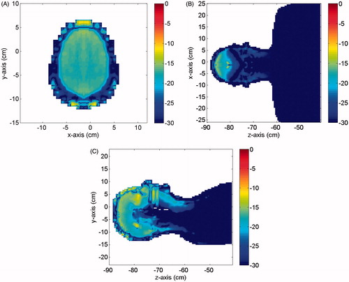
To check the accuracy of this assumption we have evaluated the relative variation of the electric power distributions (normalised to (Hf)²) at the extremes of the investigated band, f₁ = 50 kHz and f₂ = 200 kHz, namely: (13) where q_e1 and q_e2 are the aforementioned power distributions at f₁ and f₂, respectively. Figure 3 shows Δq_e(r) (in dB) in three different cut planes. As can be seen, apart from a few hot spots located on the skin layer, where the error reached a value of −8 dB, a relative error not larger than about −13 dB, i.e. about 5%, was observed, which is within the accuracy for the knowledge of the values of the electric properties of the human tissues over the investigated frequency range, thus confirming the validity of our assumption.

Figure 3. Relative error in dB between the normalised (to Hf) electric power distributions dissipated in the numerical phantom at f₁ = 50 kHz and f₂ = 200 kHz. (A) Cut in the xy plane, (B) cut in the zx plane; (C) cut in the yz plane.

Optimal values of p_h, p_e and Hf

Once T_Δh(r), T_Δe(r), T_Δm(r) and T_Δext(r) were determined through the electromagnetic and thermal co-simulations described above, p_hopt and p_eopt and the corresponding Hf were estimated by using, in order, Equations 10–11 and 4(4) . The results, obtained by assuming a uniform distribution of the MNPs in the tumour and two values of T_ext, 25 °C and 30 °C, are summarised in Table 3. The following comments are in order. First, the required p_hopt grows as the tumour’s size decreases. This is an expected result and reflects the higher capability of smaller tumours to exchange heat with the surrounding tissue, due to the higher surface-to-volume ratio. Second, p_eopt, hence Hf, increases as T_ext decreases. This is also an expected result and is due to the fact that the lower T_ext is, the higher the thermal exchange from the body towards the external environment, and so the higher the amount of electric power which can be dissipated in the body, while keeping the temperature rise in the healthy tissue below the safety threshold. On the contrary, p_hopt is practically insensitive to the value of T_ext. This is due to several factors such as the tumour position, distance from the skin layer, the small tumour size, and the high blood perfusion characterising the brain tissue. Third, the lowest value for Hf is obtained for case 3, namely for deep tumours in the brain. This result is consistent with the fact that for deeper tumours the portion of head being exposed to the applied EF is larger, so that the value of z in Equation 4(4) is larger. Consequently, according to Equation 4(4) , we get a lower value of Hf. Nevertheless, in all the cases analysed a value of Hf significantly larger than the empirical threshold of 4.85 × 10⁸ A/m/s, was obtained. Accordingly, our analysis confirms, also in the more challenging and clinically relevant case of brain tumours, that this constraint is too stringent and can be relaxed, thus enabling a reduction in the amount of MNPs to be administered. On the other hand, our analysis also shows that the empirical value of 5 × 10⁹ A/m/s, adopted in the estimations reported [37], is too large for safe treatment of brain tumours. Of course, larger values of Hf may be obtained if wider transition regions and/or a less stringent safety threshold, T₂, are assigned (for brevity, data not reported). Anyway, the key point to be stressed is that the value Hf to be used in MNPH cannot be assigned heuristically, but must be established by means of a rigorous criterion, such as that considered herein.

Table 3. Optimal values for p_h, p_e and Hf: MNPs uniformly distributed in the tumour.

		Text = 25 °C			Text = 30 °C
Case	Tumour size (mm)	phopt (kW/m^3)	peopt (kW/m^3)	Hf (A/m/s)	phopt (kW/m^3)	peopt (kW/m^3)	Hf (A/m/s)
1	20	569	1.84	1.77 × 10^9	572	1.71	1.71 × 10^9
	15	687	1.81	1.77 × 10^9	691	1.69	1.71 × 10^9
2	20	593	1.45	1.63 × 10^9	594	1.31	1.55 × 10^9
	15	687	1.45	1.62 × 10^9	689	1.31	1.54 × 10^9
3	20	611	1.46	1.13 × 10^9	611	1.36	1.10 × 10^9
	15	739	1.52	1.15 × 10^9	733	1.43	1.11 × 10^9

Optimal values of H, f and d

The optimal H, f and d, as well as the corresponding c_min estimated from p_hopt, p_eopt and Hf in Table 3, are reported in Table 4. We reported the results obtained by using Equations 1(1) and 2(2) , averaged over the MNP size distribution, here assumed lognormal. Therefore, the estimated d_opt represents the mean values of such distribution. Furthermore, a MNP size not larger than 100 nm was considered in our study, this being the maximum size defining the nanoscale range.

Table 4. Optimal values for H, f, d and c_min: MNPs uniformly distributed in the tumour.

			Text=25 °C					Text=30 °C
Case	Tumoursize (mm)	Hopt (kA/m)	fopt (kHz)	dopt (nm)Eq. (1)(1) Eq. (2)(2)		cmin (mg/mL) Eq. (1)(1) Eq. (2)(2)		fopt (kHz)	dopt (nm)Eq. (1)(1) Eq. (2)(2)		cmin (mg/mL) Eq. (1)(1) Eq. (2)(2)
1	20	10	177	17	10	8.9	12.6	171	17	10	9.2	13.2
		15	118	17	100	7.5	5.6	114	17	100	7.8	5.8
		20	89	17	70	6.9	5.5	85	17	70	7.2	5.7
	15	10	177	17	10	10.7	15.2	171	17	10	11.2	15.9
		15	118	17	100	9	6.8	114	17	100	9.4	7.1
		20	89	17	70	8.4	6.7	85	17	70	8.7	6.9
2	20	10	163	17	10	10	14.3	155	17	10	10.6	15.1
		15	109	17	100	8.4	6.4	103	17	100	8.9	6.7
		20	81	18	70	7.8	6.3	77	18	70	8.2	6.6
	15	10	162	17	10	11.7	16.7	154	17	10	12.3	17.6
		15	108	17	100	9.8	7.4	102	17	100	10.4	7.8
		20	81	18	70	9.1	7.2	77	18	70	9.6	7.7
3	20	10	113	17	10	14.6	21.2	110	17	10	15.1	21.9
		15	76	18	100	12.2	9.4	73	18	100	12.6	9.7
		20	57	18	70	11	9.2	55	18	70	11.4	9.6
	15	10	115	17	10	17.5	25.4	111	17	10	17.8	25.9
		15	76	18	100	14.7	11.3	74	18	100	14.9	11.5
		20	57	18	70	13.3	11.1	56	18	70	13.5	11.3

Concerning the MF, it turns out that for both Equations 1(1) and 2(2) , H_opt is the maximum MF, H_max, that the exposure system can produce at the tumour’s position (see the second section). Here we have considered three possible values for H_max, namely 10, 15, 20 kA/m, which are comparable with those actually achievable with the exposure systems currently employed in the clinical trials [38]. The corresponding f_opt are obtained by replacing H_max into Equation 4(4) , or equivalently by using the values of Hf in Table 3. Also for f_opt, the values obtained are within the investigated frequency range 50–200 kHz and are comparable with those characterising the aforementioned exposure systems [38].

Concerning d_opt, depending on the adopted model for the magnetic losses, completely different values are obtained. Diameters of about 17–18 nm are obtained by using Equation 1(1) , which are in satisfactory agreement with the experimental data reported [39–41]. On the contrary, a wide range of values, from 10 to 100 nm, is obtained by using Equation 2(2) , in dependence of the value of H_max. This is due to the fact that, while for H_max = 10 kA/m the equation 1.43Hc (d_opt) = H_max only has one root, (i.e. d_opt ≈ 10 nm) for H_max = 15–20 kA/m it has two roots (see Figure 1): the first in the superparamagnetic range (d_opt ≈ 10–12 nm); the second in the ferromagnetic range (d_opt ≈ 70–100 nm). Moreover, it can be seen from the behaviour of H_c(d) in Figure 1 that the slope of H_c(d) in the superparamagnetic range is higher than the slope in the ferromagnetic range. This latter aspect, while unessential in the case of mono-dispersed MNPs, plays a crucial role in the realistic case of poly-dispersed MNPs, such as those considered in this study, since it makes it the second root less sensitive than the first to deviations of d from d_opt. In other words, for a given degree of poly-dispersivity, the deviation from the optimal condition 43H_c(d_opt) = H_max is much more pronounced for the first root than the second. As a result, when H_max is high enough that two distinct values of d_opt satisfy the equation 43H_c(d_opt) = H_max, according to Equation 2(2) , the true d_opt is in the ferromagnetic range, as shown in Table 4. Anyway, the above results emphasise that one of the main challenges towards an optimised MNPH treatment is to derive a unique and reliable model able to accurately describe MNP losses over the whole range of MF amplitudes, frequencies and MNP sizes of interest. Obviously, the reliability of any model requires an extensive experimental check of its validity.

Coming to c_min, unlike d_opt, quite similar values of c_min are obtained with Equations 1(1) and 2(2) . In both cases, c_min decreases as the MF amplitude or the tumour size increases or the degree of poly-dispersivity of the MNPs decreases (data not reported for the sake of brevity). The first trend is in agreement with the predictions of the proposed criterion; the second trend is due to the decrease of p_hopt as the tumour size increases, discussed in the previous section; the third trend can be explained by noting that the lower the poly-dispersivity, the higher the fraction of MNPs with size close to the optimal. From Table 4 one can also notice that c_min increases for the deepest tumour in the brain (see case 3). This result is due to the reduction of the usable product Hf, discussed in the previous section.

Finally, we would like to point out that the values found for c_min by using Equation 1(1) are larger than those found in [14,15]. This is in part due to the more accurate dissipation model herein adopted, which takes into account the saturation effect of the magnetisation of the MNPs, completely disregarded in Bellizzi et al. [14,15]. Since the saturation effect of the magnetisation of the MNPs is actually observed at high MF amplitudes, the results found herein are expected to be more realistic than those in Bellizzi et al. [14,15]. Anyway, values of c_min less than 10 mg of MNPs/mL of tumour are still obtained. These values, smaller than those typically quoted in the literature for the treatment of tumour of comparable or even larger sizes [8–10,42–43], confirm that the application of the proposed criterion may significantly improve MNPH performances.

Numerical validation of the criterion

Once H_opt, f_opt, d_opt and c_min were determined we repeated the electromagnetic-thermal co-simulations by assigning such values to the MF and MNP parameters (the presence of the MNPs was simulated by introducing into the tumour proper magnetic losses). The aim is to verify that the temperature rise actually meets the imposed constraints 6a and 6b (in this case all the heat sources act simultaneously).

In Figure 4 we show, for each case in Table 2, and a tumour of 15 mm in size (diameter), the temperature distributions obtained in three orthogonal cuts crossing the tumour centre, when T_ext = 25 °C. Similar results, not reported for brevity, were obtained for a 20-mm tumour, as well as when T_ext = 30 °C. From the Figures one can see that in all cases the temperature of the tumour (the smallest black circle in the insets) is above the prescribed therapeutic value of 42 °C. Therefore, requirement (6a) is completely fulfilled. As expected, a significantly higher temperature, about 47–48 °C, is reached at the tumour centre. This is good from a therapeutic point of view, since the most internal cancerous cells of the tumour mass are usually the most resistant to drugs.

Figure 4. Temperature distribution induced over the irradiated tissues (MNPs uniformly distributed in the tumour). Parts (D)–(F) shows the results for case 1: (A) cut in the xy plane, (B) cut in the yz plane, (C) cut in the zx plane. Parts (D)–(F) shows the results for case 2: (D) cut in the xy plane, (E) cut in the yz plane, (F) cut in the zx plane. Parts (G)–(I) shows the results for case 3: (G) cut in the xy plane, (H) cut in the yz plane, (I) cut in the zx plane. The insets show a zoom of the tumour (smallest black circle) and the transition region (largest black circle).

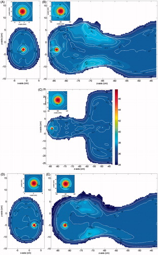
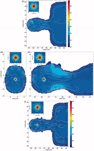
One can also notice that in all the healthy tissue outside the transition region (the largest black circle in the insets) the temperature is not higher than the safety threshold of 39 °C, as prescribed. Actually, the temperature rapidly decreases far from the tumour centre and reaches values well below 39 °C outside the transition region in the xy and xz cut planes. This behaviour is due to the high blood perfusion characterising the brain tissue which, while on the one hand makes the tumour heating harder, on the other hand makes the heating much more selective than required [14]. However, this does not happen everywhere, as can be seen in the yz cut planes, which show two secondary peaks near to the oral cavities and near to the nape. These peaks are due to the higher electric conductivity and the lower blood perfusion of these regions of the body. Anyway, both peaks are no larger than 39 °C, as prescribed by condition 6b. Moreover, no overheating is observed within the transition region. Accordingly, the results obtained confirm the reliability of the proposed criterion and show that its application allows the planning of the temperature distribution over the irradiated tissues, thus avoiding useless and harmful overheating in the healthy tissues and assuring a safe treatment.

Influence of a non-uniform MNP distribution in the tumour

To assess the influence of a more realistic, i.e. non-uniform, spatial distribution of MNPs in the tumour, we have applied the criterion by assuming a Gaussian distribution of MNPs in the tumour, which is the distribution one would obtain by injecting the MNPs at the tumour centre in the case of isotropic spread of the MNPs in the neighbouring tissue [44]. Of course, more complicated distributions are obtained in practice, depending on the tumour shape and size, the tissue heterogeneity, the rate of infusion of the MNPs, and the number and sites of injections. If needed, this can be accurately determined through a CT scan of the tumour region [45], and hence effectively taken into account in the criterion for a more reliable estimation of H_opt, f_opt, d_opt and c_min, and of the tumour heating.

As a representative example, let us consider case 1 in Table 2, with a tumour size of 15 mm. The assumed normalised radial profile of the MNP distribution in the tumour is shown in Figure 5. As can be seen, we have considered a case where a part of the injected MNPs spreads out into the healthy tissue surrounding the tumour. The results, obtained for T_ext = 25 °C, are summarised in Table 5. Since p_e depends weakly on the MNP distribution in the tumour, p_eopt, and consequently H_opt, f_opt and d_opt, is practically unchanged with respect to the case of uniformly distributed MNPs. The quantities mainly affected by the MNP distribution are p_hopt, c_min and the maximum temperature, say T_max, reached in the tumour. As can be seen, there is a marginal increase of p_hopt, hence of c_min, required to fulfil the temperature constraints 6a and 6b as compared to the uniform case. Coherently, we get a larger T_max, 48.6 °C against 47.9 °C, as obtained for the uniform case. Accordingly, the c_min increase is irrelevant, so the influence of the MNP distribution can be safely ignored, at least for the MNP spatial distribution and tumour size considered.

Figure 5. Normalised radial profile of the MNP distribution in the tumour.

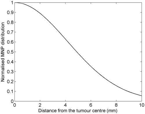
Table 5. Optimal vales for H, f, d and c_min: MNPs non-uniformly distributed in the tumour (T_ext = 25 °C).

						dopt (nm)		cmin (mg/mL)
Case	Tumour size (mm)	phopt (kW/m^3)	Hf (A/m/s)	Hopt (kA/m)	fopt (kHz)	Eq. 1	Eq. 2	Eq. 1	Eq. 2	Tmax (°C)
1	15	713	1.75 × 10^9	10	175	17	10	11.2	16	48.6
				15	117	17	100	9.4	7.2	48.6
				20	87	18	70	8.6	7	48.6

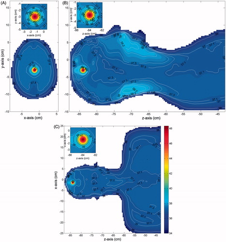
Finally, in Figure 6 we report the temperature field obtained in three orthogonal cuts through the tumour centre. As can be seen, also in this case the temperature constraints are also completely fulfilled.

Figure 6. Temperature distribution induced over the irradiated tissues (MNPs non-uniformly distributed in the tumour), for case 1 and T_ext = 25 °C: (A) cut in the xy plane, (B) cut in the yz plane, (C) cut in the zx plane. The insets show a zoom of the tumour (smallest black circle) and the transition region (largest black circle).

Validation of the criterion by using experimental SAR data

By using the experimental results on the SAR for iron oxide MNPs available in literature, we have provided a preliminary validation of the proposed criterion. In this respect, we have applied the results in Malik et al. [21] to the case in Table 5. Notably, the MNPs investigated in Malik et al. [21] are commercially available magnetite nanoparticles suspended in water, with a core size (15 nm) close to the estimated optimal, and the ranges of magnetic field amplitudes and frequencies therein considered nearly cover those of our work (10–20 kA/m and 50–200 kHz). The results obtained are reported in Table 6. The selected values of H and f are those used in Malik et al. [21] such that the product Hf is as close as possible to the numerically estimated safety threshold of 1.75 × 10⁹ of A/m/s (see Table 5). The reported values of SAR are those measured in Malik et al. [21] in correspondence to the aforementioned values of H and f, while c_min is the required therapeutic concentration of MNPs corresponding to such values of SAR. As can be seen, there is good agreement between the c_min in Table 6 and those in Table 5, obtained using Equation 1(1) , thus confirming the reliability of such a model for the SAR, at least for what concerns the class of MNPs investigated in Malik et al. [21].

Table 6. Optimal values for H, f, d and c_min by using the experimental SAR in Malik et al. [21] (T_ext = 25 °C).

Case	Tumour size (mm)	Phopt (W/cm^3)	Hf (A/m/s)	H (kA/m)	f (kHz)	dopt (nm)	SAR (W/g)	cmin (mg/mL)	Tmax (°C)
1	15	0.713	1.75 × 10^9	10.5	166	15	62.5	11.4	48.6
				16	110	15	84	8.5	48.6

Clinical scalability

As a conclusive study, by using the proposed criterion we analysed the clinical scalability of the MNPH for the case of brain tumours, namely the minimum tumour size which can be safely and effectively treated through MNPH. Since this limit depends on the MNP concentration delivered to the tumour, we first evaluated, for decreasing tumour size, c_min required for achieving the desired therapeutic heating. Then we considered the minimum tumour size such that c_min ≤ c_lim, c_lim is the maximum MNP concentration achievable in the tumour with the administration route employed.

The analysis was carried out considering tumours of spherical shape, with a size ranging from 5 to 20 mm and uniformly distributed MNPs. Tumours at the three different positions listed in Table 2 were considered in order to assess how the tumour depth affects the minimum size successfully treatable. The temperature constraints imposed and the MNP physical parameters are again those used to obtain the results in Table 3 (see the second section). Furthermore, we have assumed an intensity of 20 kA/m for the applied MF at the tumour location.

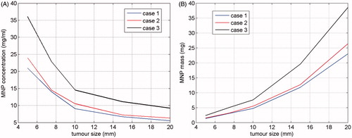
Figure 7(A) shows the behaviour of c_min versus the tumour size, for each of the positions in Table 2. For the sake of brevity, we have reported only the results obtained by using Equation 1(1) and T_ext = 25 °C (quite similar MNP concentrations were obtained by using Equation 2(2) ). As expected, c_min decreased as the tumour size increased, and the curve relative to case 3, i.e. that relative to the deepest tumour in the brain, is the highest, thus confirming that the deeper the tumour the harder is its heating. Coming to the clinical scalability, by assuming c_lim ≈ 10 mg/mL, i.e. a MNP concentration which can be actually attained inside the tumour via active biochemical targeting [46], the minimum tumour size safely and effectively treatable is about 10 mm for tumours not deeply sited in the brain. This size doubles for deep tumours. Obviously, tumours of smaller size may be treated if larger c_lim can be delivered, as happens when the MNPs are directly injected into the tumour. In this case, the treatment of smaller tumours may be even more favourable since it requires a smaller amount (i.e. total mass) of MNPs, as shown in Figure 7(B) where we report, as a function of the tumour size, the minimum amount of MNPs required for a safe and effective treatment, estimated by multiplying c_min in Figure 7(A) by the tumour volume. Of course, when the MNPs are directly injected they do not remain localised but spread into the surrounding tissue, lowering the actual concentration and enlarging the region occupied by the MNPs. However, since in the case of small tumours we can accept the heating of part of the neighbouring tissue too, and the influence of the MNP distribution is not substantial (see previous subsection), from Figure 7B we realised that the consequences of the MNPs spreading can be counteracted by a modest increase in the amount of MNPs. Hence, we conclude that in the case of directly injected MNPs, there is no lower limit to the size of treatable tumours. Of course, the estimation of the required MNPs amount would require the knowledge of how they spread into the surrounding tissues.

Figure 7. Required MNPs concentration (A) and MNPs total mass (B) for successfully heating tumors of different sizes, for each of the three positions in Table 2.

Conclusions

In this paper the feasibility and the reliability of the optimisation criterion presented in Bellizzi et al. [14], for the optimal choice of the operative conditions in MNPH, was numerically assessed with reference to the challenging and clinically relevant case of brain tumours, by using a 3D realistic model of human head.

The results of the exhaustive analysis performed have shown in this challenging case too, that the application of the criterion allows the determining of the MF and MNP features which assure the complete attainment of the therapeutic goal while minimising the required MNP dosage. Moreover, its application assures a preliminary control of the temperature rise of the exposed tissue, thus avoiding useless and harmful overheating of the healthy tissues and enabling safe treatment.

The estimation of the optimal MF parameters has shown that in all the considered cases the allowable values of Hf are larger than the safety threshold of 4.85 × 10⁸ A/m/s usually considered in the literature. Accordingly, our calculation shows that in most of the cases this constraint was too stringent and could be relaxed with a consequent reduction of the effective dosage of MNPs to be administered.

It was shown that the optimal MNP size is strongly affected by the nature of the magnetic losses. For MNPs in a stable single-domain state the optimal sizes are around 17–18 nm, when relaxation losses dominate. In contrast, when the hysteresis losses dominate, the optimal size is strongly dependent on the MF amplitudes. For amplitudes smaller than 10 kA/m, the optimal MNP size is in the superparamagnetic range, i.e. about 10 nm; for larger MF amplitudes the optimal size is in the ferromagnetic range, i.e. 70–100 nm, thus confirming that when a MF with high amplitude is used, the most efficient MNPs are those with multi-domain core.

In contrast, the required MNP concentrations are not heavily affected by the type of losses. They decrease when the MF amplitude or the tumour size increase, and increase for deep tumours. Moreover, for the degree of MNP size dispersion considered, concentrations smaller than 10 mg/mL of tumour are, in some cases, sufficient to achieve the therapeutic goal with the required heating selectivity.

A preliminary experimental validation of the criterion, by using experimental SAR available in the literature, was also provided, confirming the validity of the numerical estimations, at least for what concern the SAR of the MNPs.

Finally, a study of the clinical scalability of the MNPH has also been performed, showing that tumours larger than 10 mm in size can be successfully treated with concentrations lower than 15 mg/mL.

In conclusion, the application of the criterion could significantly improve the MNPH performance, by reducing the required MNP dosage and enabling, at the same time, a complete planning of the temperature rise of the exposed tissue. Accordingly, the proposed criterion may represent a very helpful tool for a safe, effective and optimised planning of MNPH treatments.

Disclosure statement

The authors report no conflicts of interest. The authors alone are responsible for the content and writing of the paper.

References

- Jordan A, Scholz R, Maier-Hauff K, Johannsen M, Wust P, Nadobny J, et al. Presentation of a new magnetic field therapy system for the treatment of human solid tumors with magnetic fluid hyperthermia. J Magn Magn Mater 2001;225:118–26.
- Jordan A, Wust P, Fähling H, John W, Hinz A, Felix R. Inductive heating of ferrimagnetic particles and magnetic fluids: Physical evaluation of their potential for hyperthermia. Int J Hyperthermia 2009;25:499–511.
- Hilger I. In vivo applications of magnetic nanoparticle hyperthermia. Int J Hyperthermia 2013;29:828–34.
- Johannsen M, Gneveckow U, Eckelt L, Feussner A, Waldofner N, Scholz R, et al. Clinical hyperthermia of prostate cancer using magnetic nanoparticles: Presentation of a new interstitial technique. Int J Hyperthermia 2005;21:637–47.
- Wust P, Gneveckow U, Johannsen M, Bohemer D, Henkel T, Kahmann F, et al. Magnetic nanoparticles for interstitial thermotherapy – feasibility, tolerance and achieved temperatures. Int J Hyperthermia 2006;22:673–85.
- Johannsen M, Gneveckow U, Thisien B, Taymoorian K, Cho C, Waldofner N, et al. Thermotherapy of prostate cancer using magnetic nanoparticles: Feasibility, imaging, and three-dimensional temperature distribution. Eur Urol 2007;52:1653–62.
- Maier-Hauff K, Rothe R, Scholz R, Gneveckow U, Wust P, Thisien B, et al. Intracranial thermotherapy using magnetic nanoparticles combined with external beam radiotherapy: Results of a feasibility study on patients with glioblastoma multiforme. J Neurooncol 2007;81:53–60.
- Thisien B, Jordan A. Clinical applications of magnetic nanoparticles for hyperthermia. Int J Hyperthermia 2008;24:467–74.
- Maier-Hauff K, Ulrich F, Nestler D, Niehoff H, Wust P, Thisien B, et al. Efficacy and safety of intratumoral thermotherapy using magnetic iron-oxide nanoparticles combined with external beam radiotherapy on patients with recurrent glioblastoma multiforme. J Neurooncol 2011;103:317–24.
- Matsumine A, Takegami K, Asanuma K, Matsubara T, Nakamura T, Uchida A, Sudo A. A novel hyperthermia treatment for bone metastases using magnetic materials. Int J Clin Oncol 2011;16:101–8.
- Kozissnik B, Bohorquez A, Dobson J, Rinaldi C. Magnetic fluid hyperthermia: Advances, challenges, and opportunity. Int J Hyperthermia 2013;29:706–14.
- Dutz S, Hergt R. Magnetic particle hyperthermia – a promising tumour therapy? Nanotech 2014;25:452001.
- Huang H, Hainfeld J. Intravenous magnetic nanoparticle cancer hyperthermia. Int J Nanomed 2013;8:2521–32.
- Bellizzi G, Bucci OM. On the optimal choice of the exposure conditions and the nanoparticle features in magnetic nanoparticle hyperthermia. Int J Hyperthermia 2010;26:389–403.
- Bellizzi G, Bucci OM, Di Bernardo A. Determining the optimal operative conditions in magnetic nanoparticle hyperthermia. Paper presented at the Sixth European Conference on Antennas and Propagation, Prague, 26–30 March 2012.
- Zubal IG, Harrell CR, Smith EO, Rattner Z, Gindi G, Hoffer PB. Computerized 3-dimensional segmented human anatomy. Med Phys 1994;21:299–302.
- Pearce J, Giustini A, Stigliano R, Hoopes PJ. Magnetic heating of nanoparticles: The importance of particle clustering to achieve therapeutic temperatures. J Nanotechnol Eng Med 2014;4: 0110071–14.
- Rosensweig RE. Heating magnetic fluid with alternating magnetic field. J Magn Magn Mater 2002;252:370–4.
- Fortin J, Wilhelm C, Servais J, Menager C, Bacri J, Gazeau F. Size-sorted anionic iron oxide nanomagnets as colloidal mediators for magnetic hyperthermia. J Am Chem Soc 2007;129:2628–35.
- Gonzales-Weimuller M, Zeisberger M, Krishnan K. Size-dependant heating rates of iron oxide nanoparticles for magnetic fluid hyperthermia. J Magn Magn Mater 2009;321:1947–50.
- Malik V, Goodwill J, Mallapragada S, Prozorov T, Prozorov R. Comparative study of magnetic properties of nanoparticles by high-frequency heat dissipation and conventional magnetometry. IEEE Magn Lett 2014;5:1–4.
- Shah R, Davis T, Glover A, Nikle D, Brazel C. Impact of magnetic field parameters and iron oxide nanoparticle properties on heat generation for use in magnetic hyperthermia. J Magn Magn Mater 2015;387:96–106.
- Garaio E, Sandre O, Collantes J, Garcia J, Mornet S, Plazaola F. Specific absorption rate dependence on temperature in magnetic field hyperthermia measured by dynamic hysteresis losses (AC magnetometry). Nanotech 2015;26:015704–22.
- Etheridge ML, Bischof CJ. Optimizing magnetic nanoparticle based thermal therapies within the physical limits of heating. Ann Biomed Eng 2013;41:78–88.
- Hergt R, Dutz S, Roder M. Effect of size distribution on hysteresis losses of magnetic nanoparticles for hyperthermia. J Phys Condens Matter 2008;20:1–12.
- Bordelon DE, Cornejo C, Grüttner C, Westphal F, DeWeese TL, Ivkov R. Magnetic nanoparticle heating efficiency reveals magneto-structural differences when characterized with wide ranging and high amplitude alternating magnetic fields. J Appl Phys 2011;109:124904.
- Eberbeck D, Kettering M, Bergemann C, Zirpel P, Hilger I, Trahms L. Quantification of the aggregation of magnetic nanoparticles with different polymeric coatings in cell culture medium. J Phys D Appl Phys 2010;43:405002–10.
- Etheridge ML, Hurley KR, Zhang J, Jeon S, Ring HL, Hogan C, et al. Accounting for biological aggregation in heating and imaging of magnetic nanoparticles. Technology 2014;2:214–228.
- Bellizzi G, Bucci OM. A novel measurement approach for the broadband characterization of diluted water ferrofluids. IEEE Trans Magn 2013;49:2903–12.
- Gabriel S, Lau RW, Gabriel C. The dielectric properties of biological tissues: III. Parametric models for the dielectric spectrum of tissues. Phys Med Biol 1996;41:2271–93.
- Arkin H, Xu LX, Holmes KR. Recent developments in modeling heat transfer in blood perfused tissues, IEEE Trans Biomed Eng 1994;41:97–107.
- Song CW. Effect of local hyperthermia on blood flow and microenvironment: A review. Cancer Res 1984;44: S4721–S30.
- Bellizzi G, Bucci OM. Criterion for the optimal choice of the operative conditions in magnetic nanoparticle hyperthermia: Uncertainty analysis. 19th Riunione Nazionale di Elettromagnetismo, Rome, 10–14 September 2012.
- Diller KR, Valvano JW, Pearce JA. Bioheat transfer. In: Goswami DY, ed. The CRC handbook of mechanical engineering. Boca Raton, FL: CRC Press, 2004, pp. 278–357.
- de Dear RJ, Arens E,·Hui Z, Oguro M. Convective and radiative heat transfer coefficients for individual human body segments. Int J Biometeorol 1997;40:141–56.
- Malaescu I, Marin CN. Study of magnetic fluids by means of magnetic spectroscopy. Physica B 2005;365:134–40.
- Hergt R, Dutz S. Magnetic particle hyperthermia – biophysical limitations of a visionary tumour therapy. J Magn Magn Mater 2007;311:187–92.
- Gneveckow U, Jordan A, Scholz R, Brüß V, Waldöfner N, Ricke J, et al. Description and characterization of the novel hyperthermia-and thermoablation-system MFH® 300F for clinical magnetic fluid hyperthermia. Med Phys 2004;31:1444–51.
- Gazeau F, Lévy M, Wilhelm C. Optimizing magnetic nanoparticle design for nonothermotherapy. Nanomedicine 2008;3:831–44.
- Hergt R, Dutz S, Muller R, Zeisberger M. Magnetic particle hyperthermia: Nanoparticle magnetism and materials development for cancer therapy. J Phys Condens Matter 2006;18:S2919–S34.
- Glockl G, Hergt R, Zeisberger M, Dutz S, Nagel S, Weitschies W. The effect of field parameters, nanoparticle properties and immobilization on the specific heating power in magnetic particle hyperthermia. J Phys Condens Matter 2006;18:S2935–S49.
- Pankhurst QA, Connolly J, Jones SK, Dobson J. Applications of magnetic nanoparticles in biomedicine. J Phys D Appl Phys 2003;36:R167–81.
- Leslie-Pelecky DL, Labhasetwar V, Kraus RH. Nanobiomagnetics. In: Sellmyer DJ, Skomski R, eds. Advanced magnetic nanostructures. New York: Springer, 2006, pp. 461–90.
- Golneshan A, Lahonian M. Diffusion of magnetic nanoparticles in a multi-site injection process within a biological tissue during magnetic fluid hyperthermia using lattice Boltzmann method. Mech Res Commun 2011;38:425–30.
- LeBrun A, Manuchehrabadi N, Attaluri A, Wang F, Ma R, Zhu L. MicroCT image-generated tumour geometry and SAR distribution for tumour temperature elevation simulations in magnetic nanoparticle hyperthermia. Int J Hyperthermia 2013;29:730–8.
- Leuschner C, Kumar CS, Hansel W, Soboyejo W, Zhou J, Hormes J. LHRH-conjugated magnetic iron oxide nanoparticles for detection of breast cancer metastasis. Breast Cancer Res Treat 2006;99163–76.