Simulation of respiratory motion during IMRT dose delivery

Abstract

Background. When intensity modulated radiation therapy (IMRT) is realised with dynamic multi-leaf collimators (MLC) and given under respiratory motion, dosimetric errors may occur. These errors are a consequence of the dose blurring and the interplay between the organ motion and the leaf motion. In the present study, a model for evaluating these dosimetric effects for patient-specific cases has been developed and tested. Material and methods. In the purpose written software, three dimensional (3D) dose distributions can be calculated both with and without a generated breathing cycle. To validate the presented model and illustrate its application, periodic breathing cycles were generated, where the starting phase was set randomly for each field during the calculations. Respiration in the anterior-posterior (AP), superior-inferior (SI) and left-right (LR) direction was tested and verified. To illustrate the application of the presented model, two 5-fields IMRT plans with different complexity were calculated with a 2 cm peak-to-peak motion in the AP direction for one fraction and for 25 fractions. Results. The results showed that the calculation method is of good accuracy, in particular for IMRT plans consisting of several fields, where 97% of the pixels within the body fulfilled a tolerance set to 4% dose difference and 4 mm distance to agreement (DTA). For the two IMRT plans with different complexity, pronounced respiratory induced dose errors, which increased with increasing complexity, were found for both one fraction and 25 fractions, but due to the random stating phase the interplay effect was considerably reduced for the plans consisting of 25 fractions. This illustrates how the dosimetric effects will vary depending on the dose plan and on the number of fractions investigated. Conclusion. For patient specific cases, the model can with good accuracy calculate 3D dose distributions both with and without respiratory motion, and evaluate the dosimetric effects.

Intensity modulated radiation therapy (IMRT) is a widely used treatment method that offers increased dose conformity and sparing of the critical organs. This is enabled by a multi-leaf collimator (MLC) that modulates each field during the treatment. When dynamic MLC (DMLC) is used during respiratory motion, dosimetric errors may occur. These errors are caused by blurring of the dose distribution and interplay between the organ movement and the continuous movement of the MLC. A number of different investigators have shown that the respiratory induced dose errors will vary depending on the breathing amplitude, dose rate, MLC movement and velocity [1–10]. Compared with other IMRT modalities such as solid intensity modulator (SIM) and segmented MLC (SMLC), a greater interplay effect may be expected for DMLC [11]. However, it is a general view that although the dose deviations caused by the interplay effect may be of importance for single fields and fractions, the interplay effect is not dosimetric significant for a large number of fractions [1–10]. This has been explained by Bortfeld et al. [1] as a convolution effect, where the probability distribution converges towards an expected dose value if a large number of fractions are considered and the starting phase is random for each field. This expected dose value is independent of the treatment technique and is given as a weighted average of the dose distribution without motion with respect to the organ motion. Jiang et al. [5] showed in a study how the maximum dose deviations caused by the interplay effect are reduced from 30% for one field to 18% for one fraction and further to 5% for 30 fractions. Despite the reduction, a maximum dose deviation of 5% is still of importance and may vary between different patients and field parameters. As Court et al. [3] pointed out, many of these studies focus on a particular planning system with few patient cases, a limited number of fields, patient movements and MLC movements. Also, different methods to find the optimal MLC movement exist and will develop over time, giving possible alterations in the interplay effect. One such method in particular is the direct aperture based IMRT optimisation (DABO), which is described and illustrated by Tervo et al. [12] and Seppara et al. [13]. To address some of these problems, Court et al. [3] developed a tool that can analyse whether MLC sequences for individual patients will lead to dose discrepancy larger than 10% due to the interplay effect. By only evaluating whether the dose discrepancy for each field is larger or smaller than 10%, this tool does not give any three dimensional (3D) evaluation of the dose error. As also pointed out by Court, their model only focus on the interplay effect and therefore ignores the dosimetric effects caused by dose blurring. In order to better characterise the respiratory induced dose errors, an evaluation of both effects in combination are essential. The purpose of the present study was therefore to develop a model that, by calculating 3D dose distributions with and without a generated breathing cycle, enables evaluation of both dose blurring and interplay for patient specific cases. Both the validation and the application of this model are illustrated through the present study.

Materials and methods

Computational algorithm – without respiratory motion

For n_frac fractions and n_f fields, the total dose in a 3D matrix was given by the Hadamard product or entry-wise product

where k^cal is the calibration factor, n^MU is the number of monitor units and k^FSF is the field size factor given by a field f. T^TPR, I and A are matrices, with same dimension as D, containing the tissue phantom ratio (TPR), the intensity factor and the distance correction factor for each calculation point defined in the calculation matrix. This equation is based on simplified dose calculations for isocentric technique, which is described by Khan [14]. The TPR factor is dependent on both the depth (d) and the effective quadratic field size (f ^eff). The intensity factor represents the projected fluence in the iso-plane (i.e. the axial plane found at the depth of the iso-centre). The distance correction factor was given by the inverse square law, which is dependent on the distance between the calculation point and the source. At our clinic, a calibration factor of 130 MU/Gy is used and the field size factor is a product of the collimator scatter factor the phantom scatter factor.

Field parameters and defined structures were read from DICOM files exported from the treatment planning system (TPS). A two dimensional (2D) intensity distribution or fluence was calculated based on a finite number of control points, representing the position for each MLC leaf as a function of monitor units delivered. For each control point interval, the intensity profile in the iso-plane was calculated for each leaf pair as shown in Figure 1. By combining the profiles from all leaf pairs and weighting them with the dose fraction given by the investigated control point interval, a total intensity distribution was formed for each control point interval. These 2D intensity distributions were convolved with a pencil beam kernel extracted from the TPS and summed to form a final intensity distribution for each field. The pencil beam kernel was in the present study extracted from a depth equal to 10 cm. The extension of the pencil beam kernel was limited to a radius of 2.5 cm in order to reduce the calculation time. From the final intensity distributions, the intensity factors were found from the calculation points’ projection vector onto the iso-plane. This vector is dependent on iso-centre position, gantry rotation, collimator rotation and couch rotation.

Figure 1. Illustration of a fluence profile calculated for one MLC leaf pair and for one control point interval. Both leafs moves from a control point k₁ to a control point k₂, resulting in fluence profile defined for the control point interval k₁-k₂. In the open part of the field the fluence will be 1, whereas in the closed part of the field the fluence will be given by the transmission through the MLC leafs. In the partially closed field the fluence will be described through a linear gradient.

The field size factor (FSF) tables used at our clinic are based on the field size given by the primary collimator. This will be applicable to open fields, but not to IMRT fields where each field is substantially covered by the MLC leafs, which reduces the phantom scatter contribution. To account for this reduction, the effective quadratic field size (f ^eff) was used to find the FSFs as well as the TPR factors. The effective field size was in the present study set equal to the square root of the area with intensity larger than 30% of the maximum intensity. This area was found from the final intensity distribution for each field and was verified experimentally (not shown here) to give reasonable estimates of the effective field size.

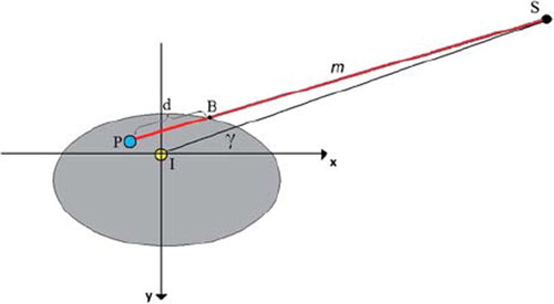
The depth (d) for each calculation point was found by considering a line m between the calculation point (P) and the radiation source (S). This line is illustrated in Figure 2 and given by Equation 2 as a function of the parameter t.

As illustrated in Figure 2, the line crosses the Body contour in a point B, giving the depth as the length of the vector . The crossing point B was found by increasing the parameter t from 0 to 1, using discrete steps corresponding to the defined pixel size in the dose matrix. For each t, it was controlled whether m(t) was inside or outside the Body contour, and in the crossing point B was defined.

Figure 2. Walking with discrete steps along a line m, defined as the line from a calculation point (P) to the radiation source (S), the depth (d) is found from the crossing point (B). The position of the radiation source is given by the gantry rotation γ around the iso-centre I.

Computational algorithm – with respiratory motion

It was assumed that the patient is breathing periodically and that the entire structure is equally affected by the breathing, i.e. organ deformation was not considered. With this simplification only structures actually affected by respiration can be evaluated. Based on previous reports, the amplitude and period was in the present study set to 1 cm and 4 s, respectively [15,16]. The starting phase was set randomly for each field, thus simulating a patient that is breathing freely throughout the treatment.

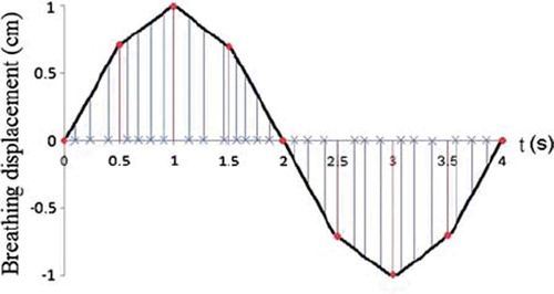
Based on the control points for each field, the dose distribution with a generated breathing cycle was calculated by correlating each control point to the radiation time. This will, as illustrated in Figure 3, result in all control points being dispersed over the breathing cycle, but not necessarily evenly. During the calculation the iso-centre was moved with discrete steps according to the displacement found from the corresponding control point intervals. In order to reduce the calculation time, each breathing period was in the present study divided into eight main intervals with assumed linearity within each interval (see Figure 3). The iso-centre position was then found for each control point interval through interpolation between the displacements found at the start and end time for the main interval covering the control points of interest. Since the centre of the calculation matrix was defined by the iso-centre, a movement of the iso-centre also caused changes in the calculation points’ depths and projection vectors onto the iso-plane. Correspondingly to the iso-centre position, the depths and the projection vectors were therefore recalculated for each displacement through interpolation between the depths and projection vectors calculated at the start and end time for the main interval. Knowing the intensity distribution for each control point interval, the total dose distribution in a 3D matrix was then found as

where n_frac, n_f, k^cal, n^MU , k^FSF, T^TPR, I and A are as described for Equation 1 without respiratory motion, and n_ctrl is the number of control points set in a field f. In contrast to the calculations without respiratory motion, the TPR factors and the distance correction factors were calculated for each control point interval. Correspondingly the intensity factors were extracted from the total intensity distribution found for each control point interval. Both the depths and the projection vectors are dependent on the starting phase set in the breathing cycle. Since the starting phase was randomised for each field during the calculations, this resulted in both the depths and the projection vectors being dependent on the fraction. The dose distribution calculated at each control point interval was summed with respect to the relative displacement of the iso-centre.

Figure 3. The breathing cycle is generated as a periodic function, where each period is divided into eight main intervals. Linearity is assumed within each interval. The control points (x), describing the position for each MLC leaf as a function of monitor units delivered, are dispersed over the breathing cycle by correlating each control point to the radiation time.

The programming tool Interactive Data Language (IDL; ITT Visual Information Solutions, USA) was used during the development of the computational algorithm. During the calculations both with and without respiratory motion, the body structure was assumed to be water equivalent. This assumption restricts the calculations to targets outside lungs, like kidney, liver, spleen and pancreas, which also have been shown to be affected by respiration [16–18]. Correction with off axis ratios has been ignored in the present study. This will be of little significance when looking at relatively small fields. In the calculation matrices a resolution of 2.5 cm was chosen for the axial-plane, whereas the resolution in the superior-inferior direction was set equal to the CT image plane separation (here 5 mm). A depth resolution of 5 mm was set in the TPR tables used in this clinic.

Validation

The treatment planning system Eclipse (Varian Medical Systems, Palo Alto, Ca, USA) was used in the present study to validate and test the algorithm. All calculations were performed with the Pencil Beam Algorithm and water equivalent phantoms. To verify dose calculations without generated respiration, a single conventional field with a field size equal to 10 × 10 cm² and gantry rotation set to 0° was created. With SSD set to 90 cm and the number of monitor units to 130 MU, the field set-up was in this plan set equal to the calibration set-up used at this clinic. To verify dose calculations with respiratory motion, a single conventional 4 × 4 cm² field with gantry rotation set to 0˚ was created. The number of monitor units was set to 133.33 MU and the dose rate to 400 MU/min, which corresponded to five whole breathing cycles when the breathing period was set to four seconds. Because the TPS is incapable to simulate the interplay effect, only the dose error caused by dose blurring was possible to verify. Since the single field was static, 100 control points was created in the presented model and evenly distributed over the radiation time in order to calculate the dose distribution as described in Equation 3. To create a basis of comparison, a simple breathing cycle was simulated in the TPS by moving the iso-centre with discrete steps. These steps corresponded to a time increment of 0.5 seconds, resulting in a plan consisting of eight fields with equal weighting, but with considerable lower time resolution compared with the resolution set in the presented model. Three simulations were performed, where the iso-centre was moved in the anterior-posterior (AP), left-right (LR) and superior-inferior (SI) direction, respectively.

The agreement between the dose distributions calculated by the presented model and dose distributions calculated by the TPS was found for the conventional fields by calculating the deviations δ₁, δ₂, δ₃ and δ₄. δ₁ is expressed as the maximal relative dose deviation for points in high dose areas but in small dose gradients, δ₂ is the maximal relative dose deviation for points outside the field in low dose areas, δ₃ is the maximal iso-dose shift for data points in the penumbra region (10–90% iso-dose), whereas δ₄ is the maximal relative dose deviation for data points on the central beam axis beyond the depth of d_max. δ₁, δ₂ and δ₃ were in the present study calculated from profiles centred on the iso-centre.

In order to validate more clinical relevant dose distributions, two 5-field IMRT plans, consisting of the same planning treatment volume (PTV) and critical organ, but with different complexity, were created. The five fields were evenly distributed around the Body with gantry rotation 0˚, 73˚, 146˚, 219˚ and 292˚. In the complex plan a high dose rate (600 MU/min) was chosen and strict demands for the critical organ. A lower dose rate (400 MU/min) and less strict demands was chosen for the less complex plan. The smoothing factor in Eclipse's optimisation algorithm was also regulated, where a low smoothing was selected for the complex plan. This resulted in approximately twice as high MU and half the average leaf pair opening in the complex plan compared with the less complex plan. Both plans were calculated without respiratory motion for 25 fractions, where each fraction was set to 2 Gy. To evaluate the agreement between the dose distributions calculated by the model and the dose distribution calculated by the TPS, the gamma index was calculated as described by Low et al. [19]. A tolerance of 4% dose difference and 4 mm distance to agreement (DTA) was used in the calculations of the gamma index. The gamma test was performed on the 2D axial-planes.

Application

To illustrate the application of the presented model, and its ability to evaluate dose errors due to interplay and blurring, the two 5-field IMRT plans created during the validation was also calculated with a 2 cm peak-to-peak motion. This example only includes a respiratory motion in the AP direction. Both plans were calculated for one fraction and 25 fractions, and each calculation was repeated three times in order to evaluate possible variations in the interplay effect. The treatment delivery duration expected for the five fields corresponded to approximately three to five whole breathing cycles.

Results

In Figure 4, a horizontal and vertical profile is shown for the conventional 10 × 10 cm² field calculated without respiratory motion. In both profiles, the dose in the calibration point placed along the central axis is 1 Gy as expected from the calibration set-up. The maximum dose deviations found in the horizontal and vertical profile are listed in Table I. As illustrated, good agreement was found in the high dose areas as well as in the penumbra region, but some disagreement was found outside the field where the software underestimated the dose.

Figure 4. Horizontal profile (a) and vertical profile (b) shown for the 10 × 10 cm² field. Both profiles are centred on the iso-centre. The dose distribution is calculated by Eclipse and by the presented model (MotionControl).

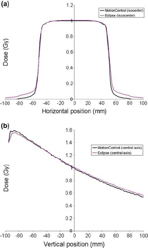
Table I. Maximum deviations calculated for a conventional 10 × 10 cm² field and for a 4 × 4 cm² field with and without a 2 cm peak-to-peak respiratory motion in the LR, SI and AP direction. The dose deviations δ₁, δ₂ and δ₄ are given relative to a reference dose of 1 Gy, whereas δ₃ is given as the shift of iso-dose lines expressed in mm.

Dose deviation	10 × 10 cm^2 field (without motion)	4 × 4 cm^2 field (without motion)	4 × 4 cm^2 field (with motion in the LR direction)	4 × 4 cm^2 field (with motion in the SI direction)	4 × 4 cm^2 field (with motion in the AP direction)
δ1 (outside central beam axis in small gradient)	0.7%	1.3%	0.2%	0.1%	0.7%
δ2 (outside field in low dose area)	5.0%	2.0%	1.8%	2.0%	1.9%
δ3 (penumbra region in dose profile)	1.6 mm	0.8 mm	1.1 mm	1.4 mm	0.6 mm
δ4 (central beam axis)	3.3%	1.2%	1.8%	2.1%	1.2%

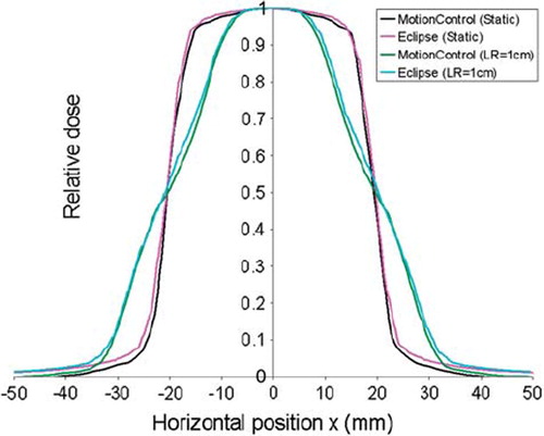
With a respiratory motion in the LR and SI direction (i.e. perpendicular to the radiation beam), the dose blurring will as illustrated in Figure 5 reduce the slope of the dose gradient. For the respiratory motion in the AP direction (i.e. parallel to the radiation beam), negligible changes in the distance correction factor and the effective field size was found. This was due to small alterations in the distance between the calculation points and the radiation source. The maximum dose deviations found for the conventional 4 × 4 cm² field calculated with and without respiratory motion in the LR, SI and AP direction, are listed in Table I. Good agreement was found in all three cases. Due to less scattered radiation, a better agreement was found outside the small field compared with the larger 10 × 10 cm² field.

Figure 5. Horizontal profiles shown for the conventional 4 × 4 cm² field after calculation of dose distributions both with and without a 2 cm peak-to-peak motion in the LR direction. The dose distributions are calculated by Eclipse and by the presented model (MotionControl), and are for both cases centred on the iso-centre.

In Figure 6, a horizontal profile is shown for the less complex 5-field IMRT plan. Table II lists the results of the gamma evaluation calculated for the complex and less complex plan in the whole body, target and critical organ, respectively. With over 97% of the pixel within the body fulfilling the gamma criteria, good calculation accuracy was shown for the presented model.

Figure 6. Horizontal profile shown for the less complex IMRT plan consisting of 5-fields. The dose distribution is calculated by Eclipse and by the presented model (MotionControl), and is centred on the iso-centre.

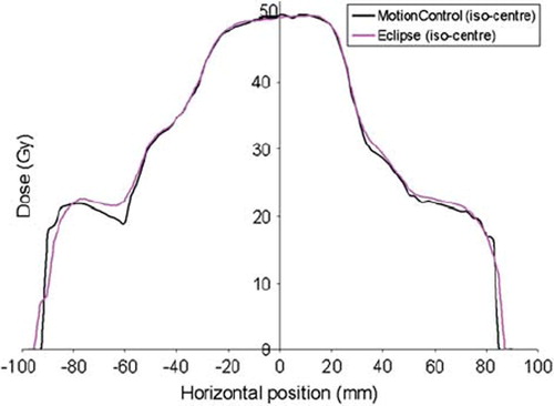
Table II. Gamma index calculated relative to the prescribed dose (50 Gy) for the complex IMRT plan and the less complex IMRT plan. A tolerance of 4% dose difference and 4 mm distance to agreement was used in the evaluation of the dose distribution calculated to the body, target and critical organ, respectively.

Volume	Gamma index<1 Less complex	Gamma index<1 Complex
Body	97.6%	97.3%
Target	100%	99.8%
Critical Organ	100%	96.3%

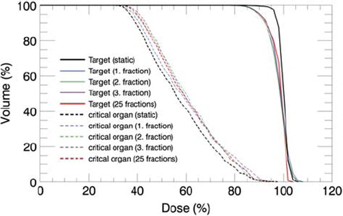
A 2 cm peak-to-peak motion in the AP direction will, as illustrated by the three single fractions in Figure 7, lead to a reduced PTV coverage and increased dose in the critical organ. Due to the random starting phase set for each field during the calculations, the dose deviations found in the three fractions were not identical. Both the localisation and the extent of the dose deviations fluctuated due to the varying interplay effect. This is illustrated in the dose profiles shown in Figure 8 for the complex IMRT plan. With both positive and negative dose deviations, these fluctuations cancelled when 25 fractions were considered. Small variations was found between the dose distributions calculated with 25 fractions in both the complex and less complex IMRT plan, indicating that dose errors due to interplay effect will be considerably reduced if the starting phase is random and the treatment plan consist of a large number of fractions. One of the three dose distributions consisting of 25 fractions is shown in Figure 8 to illustrate the cancellation of the interplay effect in the complex IMRT plan. Assuming negligible interplay effect for the dose distributions calculated for 25 fractions, the expected mean dose blurring in the target and the critical organ was calculated for both the complex and less complex IMRT plan as the mean absolute dose deviation relative to the local dose without respiratory motion. Correspondingly the largest maximum dose deviation due to interplay effect was calculated for the three single fractions as the maximum absolute dose deviation relative to the local expected dose blurring. The resulting calculations are listed in Table III. Compared with the less complex plan, larger dose errors, both due to blurring and interplay effect, was found for the complex plan. The consequence of the blurring effect is clearly illustrated in the dose volume histogram shown in Figure 9 for the complex IMRT plan. Due to reduced dose gradients at the edge of the PTV volume, the dose deviations found in the PTV is mainly found amongst the lowest doses.

Figure 7. Dose distribution illustrated in the iso-plane for the complex IMRT plan. In a) the dose distribution is calculated without respiratory motion, whereas in b)-d) the dose distribution is calculated with a 2 cm peak-to-peak motion in the AP direction for three single fractions.

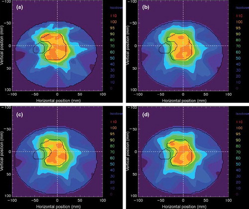
Figure 8. Horizontal profile (a) and vertical profile (b) illustrated for the same dose distributions as in Figure 7, in addition to a dose distribution calculated for 25 fractions. The profile lines are shown as with dashed lines in Figure 7 and are both centered on the iso-centre. Both the position of the target and the critical organ is illustrated for the investigated profile lines.

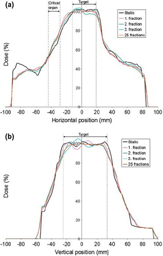
Table III. Mean expected dose blurring in the target and the critical organ, calculated for the complex and less complex plan as the mean absolute dose deviation for 25 fractions relative to the local dose without respiratory motion. Correspondingly the largest maximum dose deviation due to interplay effect is calculated as the maximum absolute dose deviation relative to the local expected dose blurring, i.e. dose distribution for 25 fractions.

	IMRT complex		IMRT less complex
Dose deviation	Target	Critical Organ	Target	Critical Organ
Mean blurring	3% ± 3%	7% ± 5%	1% ± 2%	2% ± 1%
Max interplay	9%	9%	5%	9%

Figure 9. Dose volume histogram plotted for the same dose distributions as in Figure 8. Solid lines represent the dose distribution in the PTV, whereas dashed lines represent the dose distribution in the critical organ.

Discussion

In the present study we have presented a model that successfully calculates 3D dose distributions both with and without respiratory motion for single fractions and for multiple fractions. It has also been shown that this calculation model allows for evaluation of both dose blurring and interplay for patient-specific cases.

Despite some simplifications, like limited TPR resolution, ignoring of off-axis ratios and reduced pencil beam kernel, good calculation accuracy has been shown through the validation of the calculation algorithm. Some discrepancy was found outside the single fields (see Table I), where the software underestimated the dose. This is mainly due to the reduced pencil beam kernel. Experimentally (not shown here), it was found that the dose discrepancy in low dose area decreases with increasing extension of the pencil beam kernel. However, with a larger extension of the pencil beam kernel, a correction with off-axis ratios seems necessary. At the same time it should be pointed out that the purpose for this model was not to give strictly correct dose distributions, but to give reasonable estimates of the respiratory induced dose errors. Also, an overall error reduction or smearing will take place when considering an entire plan consisting of several fields.

The results found for the two IMRT plans with different complexity are in good agreement with previous studies [1–10]. For both the complex and the less complex plan pronounced variations in the interplay effect was found for the single fractions. According to Court et al. [3], the interplay effect is divided into two orthogonal directions; parallel and perpendicular interplay, depending on whether the MLC motion is parallel or perpendicular to the organ motion. Both interplay effects may vary considerably depending on the dynamical MLC movement relative to the organ motion. Court et al. showed that the parallel interplay increases with decreasing MLC separation (distance between opposing MLC leaves) and increasing MLC speed. Correspondingly the perpendicular interplay increases with decreasing MLC separation, increasing displacement between adjacent MLCs and increasing MLC speed. These are all parameters determining a plan's complexity and will vary from patient to patient. When comparing the two IMRT plans calculated in this work, a larger interplay effect was found for the complex plan, which is in good agreement with Court et al. In both plans, the interplay effect was considerably reduced when a large number of fractions were considered and the starting phase was random for each field during the calculations. This is a consequence of the convolution effect described by Bortfeld et al. [1], where the variations in the local dose deviations are reduced with increasing number of fractions. However, it should be pointed out that also this reduction is patient- and plan-specific. Also, the dosimetric effect caused by the dose blurring may still be of importance. As illustrated in the present study, the dose blurring will as a consequence of sharper dose gradients increase with increasing complexity.

Although the calculations have in the present study been restricted to water equivalent targets, this is not a limitation for the model. By conversion to radiobiological depth, the model may be used to calculate dose distributions in lungs. For calculations in heterogeneous tissue, validation of the presented model with a different algorithm than the Pencil Beam should be considered, as this algorithm does not consider the transport of secondary electrons. In these cases, the Analytical Anisotropic Algorithm and Monte Carlo simulations will give a better basis of comparison [20,21]. By looking at the clinical target volume (CTV) coverage instead of the PTV coverage, this model may also be used to evaluate the internal margins set to account for the respiratory motion. In order to fully evaluate the internal margins it should be taken into account that random set up uncertainties may contribute to additional dose blurring [7,22]. This dose blurring can easily be simulated in the presented model through an additional iso-centre shift for each fraction during the calculations.

In the present work simple breathing cycles were generated to simulate a patient. When using the calculation model presented here, real breathing curves, registered with f. ex 4DCT, should be used. At the same time it should be stated that these breathing curves do not fully illustrate the organ motion. A patient's respiration often leads to movements in multiple directions and to deformation of organ volumes. This is not taken into account in this study, but movements in multiple directions could be included.

Different techniques, such as gating and DMLC tracking, have been introduced into the radiation oncology practice to account for respiratory motion. If the respiratory-gated treatment technique is employed, the patient is only radiated during limited parts of the breathing cycle [18], whereas in DMLC tracking the motion is compensated through reshaping of the MLC configuration [23,24]. An important application of the model presented in this study is the opportunity to control if such a treatment technique is necessary for specific targets. Also, by looking at limited parts of the breathing cycle, this model can easily calculate the expected dose distribution for treatment with gating. This may be particularly useful since the starting phase, set for each field during the treatment with gating, is fixed and not random. Depending on the size and placement of the gating window, this may lead to a systematic dose deviation due to the interplay effect, which will not cancel out by increasing the number of fractions. Interplay effect in gated IMRT is a topic that still has received little attention. Chen et al. [25] showed that the difference between measured dose in a stationary phantom and a moving phantom will increase with increasingly allowed motion in the set gating window, but no significant difference was found between the dose distributions when the gating window was set to 0.5 cm. Here one should also keep in mind that these differences will vary between different patients and MLC sequences, and that a patient's breathing curve will not be as regular as a moving phantom. The opportunity to evaluate this dosimetric effect for patient specific cases will therefore be very beneficial.

In conclusion, an algorithm has been developed that can evaluate the dosimetric effects caused by respiratory motion during an IMRT treatment for patient specific cases. The model calculates 3D dose distributions both with and without respiratory motion for single fractions as well as multiple fractions. The calculation method has been shown to be of good accuracy and enables evaluation of the dosimetric effects both due to interplay and dose blurring.

Acknowledgements

We gratefully thank Ludvig Muren for constructive feedback during the writing process.

Declaration of interest: The authors report no conflicts of interest. The authors alone are responsible for the content and writing of the paper.

References

- Bortfeld T, Jokivarsi K, Goitein M, Kung J, Jiang SB. Effects of intra-fraction motion on IMRT dose delivery: Statistical analysis and simulation. Phys Med Biol 2002;47:2203–20.
- Chui CS, Yorke E, Hong L. The effects of intra-fraction organ motion on the delivery of intensity-modulated field with a multileaf collimator. Med Phys 2003;30:1736–46.
- Court LE, Wagar M, Ionascu D, Berbeco R, Chin L. Management of the interplay effect when using dynamic MLC sequences to treat moving targets. Med Phys 2008;35:1926–31.
- Duan J, Shen S, Fiveash JB, Popple RA, Brezovich IA. Dosimetric and radiobiological impact of dose fractionation on respiratory motion induced IMRT delivery errors: A volumetric dose measurement study. Med Phys 2006;33:1380–7.
- Jiang SB, Pope C, Al Jarrah KM, Kung JH, Bortfeld T, Chen GT. An experimental investigation on intra-fractional organ motion effects in lung IMRT treatments. Phys Med Biol 2003;48:1773–84.
- Yu CX, Jaffray DA, Wong JW. The effects of intra-fraction organ motion on the delivery of dynamic intensity modulation. Phys Med Biol 1998;43:91–104.
- Bortfeld T, Jiang SB, Rietzel E. Effects of motion on the total dose distribution. Semin Radiat Oncol 2004;14:41–51.
- Seco J, Sharp GC, Turcotte J, Gierga D, Bortfeld T, Paganetti H. Effects of organ motion on IMRT treatments with segments of few monitor units. Med Phys 2007;34:923–34.
- Webb S. Motion effects in (intensity modulated) radiation therapy: A review. Phys Med Biol 2006;51:R403–25.
- Verellen D, Tournel K, Linthout N, Soete G, Wauters T, Storme G. Importing measured field fluences into the treatment planning system to validate a breathing synchronized DMLC-IMRT irradiation technique. Radiother Oncol 2006;78:332–8.
- Ehler ED, Nelms BE, Tome WA. On the dose to a moving target while employing different IMRT delivery mechanisms. Radiother Oncol 2007;83:49–56.
- Tervo J, Lyyra-Laitinen T, Kolmonen P, Boman E. An inverse treatment planning model for intensity modulated radiation therapy with dynamic MLC. Appl Math Comput 2003; 135:227–50.
- Seppala J, Lahtinen T, Kolmonen P. Major reduction of monitor units with the avoidance of leaf-sequencing step by direct aperture based IMRT optimisation. Acta Oncol 2009;48:426–30.
- Khan FM. The physics of radiation therapy. 3rd. Philadelphia: Lippincott Williams & Wilkins; 2003.
- Rietzel E, Pan T, Chen GT. Four-dimensional computed tomography: Image formation and clinical protocol. Med Phys 2005;32:874–89.
- Brandner ED, Wu A, Chen H, Heron D, Kalnicki S, Komanduri K, . Abdominal organ motion measured using 4D CT. Int J Radiat Oncol Biol Phys 2006;65:554–60.
- Xi M, Liu MZ, Li QQ, Cai L, Zhang L, Hu YH. Analysis of abdominal organ motion using four-dimensional CT. Ai Zheng 2009;28:989–93.
- Keall PJ, Mageras GS, Balter JM, Emery RS, Forster KM, Jiang SB, . The management of respiratory motion in radiation oncology report of AAPM Task Group 76. Med Phys 2006;33:3874–900.
- Low DA, Harms WB, Mutic S, Purdy JA. A technique for the quantitative evaluation of dose distributions. Med Phys 1998;25:656–61.
- Chetty IJ, Curran B, Cygler JE, DeMarco JJ, Ezzell G, Faddegon BA, . Report of the AAPM Task Group No. 105: Issues associated with clinical implementation of Monte Carlo-based photon and electron external beam treatment planning. Med Phys 2007;34:4818–53.
- Gray A, Oliver LD, Johnston PN. The accuracy of the pencil beam convolution and anisotropic analytical algorithms in predicting the dose effects due to attenuation from immobilization devices and large air gaps. Med Phys 2009;36: 3181–91.
- van Herk M, Remeijer P, Rasch C, Lebesque JV. The probability of correct target dosage: Dose-population histograms for deriving treatment margins in radiotherapy. Int J Radiat Oncol Biol Phys 2000;47:1121–35.
- Poulsen PR, Cho B, Sawant A, Ruan D, Keall PJ. Dynamic MLC tracking of moving targets with a single kV imager for 3D conformal and IMRT treatments. Acta Oncol 2010;49:1092–100.
- Sawant A, Venkat R, Srivastava V, Carlson D, Povzner S, Cattell H, . Management of three-dimensional intrafraction motion through real-time DMLC tracking. Med Phys 2008;35:2050–61.
- Chen H, Wu A, Brandner ED, Heron DE, Huq MS, Yue NJ, . Dosimetric evaluations of the interplay effect in respiratory-gated intensity-modulated radiation therapy. Med Phys 2009;36:893–903.